Quantum Quenches in the Hubbard Model: Time Dependent Mean Field Theory and The Role of Quantum Fluctuations

Abstract

We study the non equilibrium dynamics in the fermionic Hubbard model after a sudden change of the interaction strength. To this scope, we introduce a time dependent variational approach in the spirit of the Gutzwiller ansatz. At the saddle-point approximation, we find at half filling a sharp transition between two different regimes of small and large coherent oscillations, separated by a critical line of quenches where the system is found to relax. Any finite doping washes out the transition, leaving aside just a sharp crossover. In order to investigate the role of quantum fluctuations, we map the model onto an auxiliary Quantum Ising Model in a transverse field coupled to free fermionic quasiparticles. Remarkably, the Gutzwiller approximation turns out to correspond to the mean field decoupling of this model in the limit of infinite coordination lattices. The advantage is that we can go beyond mean field and include gaussian fluctuations around the non equilibrium mean field dynamics. Unlike at equilibrium, we find that quantum fluctuations become massless and eventually unstable before the mean field dynamical critical line, which suggests they could even alter qualitatively the mean field scenario.

I Introduction

Recent years have seen an enormous progress in preparing, controlling and probing ultra cold atomic gases loaded in optical lattices Bloch et al. (2008). Their high degree of tunability allows to change in time the microscopic parameters controlling interactions among atoms and to measure the resulting quantum evolution. At the same time their excellent isolation from the environment makes those systems particularly well suited to address questions related to non equilibrium phenomena in isolated many body quantum systems. These major achievements triggered a huge interest on time dependent phenomena in condensed matter systems. In this respect, the recent experimental realization of a fermionic Mott insulator Jordens et al. (2008); Schneider et al. (2008) opened the way to investigate out-of-equilibrium phenomena in strongly correlated fermionic systems Strohmaier et al. (2010).

From a more theoretical perspective these experiments offer the chance to probe strongly correlated systems in a completely novel regime. Indeed, when driven out of equilibrium, interacting quantum systems can display peculiar dynamical behaviors or even be trapped into metastable configurations that differ completely from their equilibrium counterpart Rosch et al. (2008); Rapp et al. (2010). Although actual experiments are always performed by tuning parameters at a finite rate, an useful idealization consists in a so called quantum quench Calabrese and Cardy (2006). Here the system is firstly prepared in the many-body ground state $|\Psi_{i}\rangle$ of some initial Hamiltonian $H_{i}$ which is then suddenly changed to $H_{f}\neq H_{i}$, for example by globally switching on or off some coupling constants. As a consequence of this instantaneous change the initial state $|\Psi_{i}\rangle$ turns to be an highly excited state of the final Hamiltonian. Naturally, many non trivial questions arise concerning the real-time evolution after the quantum quench. The interest on these classes of non equilibrium problems relies both on the dynamics itself, Kollath et al. (2007); Barmettler et al. (2009) as well as on the long-time properties where the question of thermalization or its lack of is still highly debated.Rigol et al. (2008); Biroli et al. (2010); Gogolin et al. (2011) This issue is not only of fundamental theoretical interest but also of great practical relevance for establishing whether and to what extent experiments on cold atoms could reproduce equilibrium phase diagrams of model hamiltonians.

The literature on quantum quenches in interacting bosonic and fermionic systems is by now very broad, see for example the recent topical reviews Eckstein, M. et al. (2009); Barmettler et al. (2010); Cazalilla and Rigol (2010); Polkovnikov et al. (2010) For what concerns strongly correlated electrons in more than one dimension, the subject is still largely unexplored and progresses have been done only very recently. The single band Hubbard model Hubbard (1963); Gutzwiller (1963); Kanamori (1963) represent one of the simplest yet non trivial models encoding the physics of strong correlations, namely the competition between electronic wave function delocalization due to hopping $t$ and charge localization due to large Coulomb repulsion $U$. Its Hamiltonian reads

$$\mathcal{H}\left(t\right)=-\sum_{\sigma}\sum_{\langle\mathbf{R},\mathbf{R^{\prime}}\rangle}\,t_{\mathbf{R}\mathbf{R^{\prime}}}\,c^{\dagger}_{\mathbf{R}\sigma}\,c^{\phantom{\dagger}}_{\mathbf{R^{\prime}}\sigma}+U\left(t\right)\sum_{\mathbf{R}}\,n_{\mathbf{R}\uparrow}\,n_{\mathbf{R}\downarrow}\,.$$ (1)

Despite the everlasting interest on its groundstate properties, theoretical investigations on the non equilibrium dynamics of this paradigmatic strongly correlated model have been started only very recently. The dynamics of Fermi system after a sudden switch-on of the Hubbard interaction has been studied firstly in Refs. Moeckel and Kehrein, 2008, 2009 using the flow-equation approach and then in Refs. Eckstein et al., 2009, 2010 using Non equilibrium Dynamical Mean Field Theory (DMFT). Results suggest the existence of two different regimes in the real-time dynamics, depending on the final interaction strength $U_{f}$. At weak coupling,Moeckel and Kehrein (2008) the systems is trapped at long-times into a quasi-stationary regime which looks as a zero temperature Fermi Liquid from the energetic point of view but features a non thermal distribution function in which correlations are more effective than in equilibrium. This pre-thermalization phenomenon has been confirmed by DMFT results,Eckstein et al. (2009) which further indicate a true dynamical transition above a critical $U_{fc}$ towards another regime with pronounced oscillations in the dynamics of physical quantities. This picture has been recently confirmed by means of a simple and flexible approximation scheme based on a proper extension of the Gutzwiller variational method  Schiró and Fabrizio (2010). Results for the time depedent mean field theory show at half filling, a sharp transition between two different regimes of small and large coherent oscillations, separated by a critical line of quenches where the system finds a fast way to relax. Away from particle hole symmetry the transition is washed out, leaving a sharp crossover visible in the dynamics and in the long-time averages of physical quantities.

The aim of the present work is twofold. From one side, we present details on the time dependent Gutzwiller method for fermions and discuss its application to the problem of an interaction quench in the single band Hubbard model. Secondly, we discuss the role of quantum fluctuations on top of the Gutzwiller dynamics. In order to do that we formulate the original Hubbard model in terms of an auxilary Quantum Ising Model in a transverse field coupled to free fermionic quasiparticle. Such a $Z_{2}$ slave spin theory, introduced in Refs. Huber and Rüegg, 2009; Rüegg et al., 2010 for the equilibrium problem, allows us to study the effect of small quantum fluctuations, both in equilibrium as well as for the non equilibrium dynamics. We notice that the role of quantum fluctuations on this mean field dynamical transition is of broader theoretical interest, as recent investigations have shown the very same phenomenon occurs in other models of interacting quantum field theories Sciolla and Biroli (2010); Gambassi and Calabrese (2010).

The paper is organized as follows. In the first part we introduce the time dependent variational method we have devised to describe non equilibrium dynamics in correlated electrons systems. Section II is devoted to a general formulation while section III to the study of quantum quenches in the single band fermionic Hubbard Model. In the second part of the paper we broaden the perspective and formulate the Hubbard model in terms of auxiliary Quantum Ising Model coupled to free fermionic quasiparticles. In section IV we show how the mapping works and how to recover the Gutzwiller results. Section IV.4 is devoted to the role of quantum fluctuations. Finally section V is for conclusions.

II A General Formulation

We assume a system of interacting electrons that is initially in a state with many-body wavefunction $|\Psi_{0}\rangle$. For times $t>0$, $|\Psi_{0}\rangle$ is let evolve with the Hamiltonian $\mathcal{H}$, which could even be explicitly time-dependent. We shall assume that short range correlations are strong either in the initial wavefunction, or in $\mathcal{H}$, or in both. The goal is calculating average values of operators during the time evolution. Because of interaction, a rigorous calculation is unfeasible, so that an approximation scheme is practically mandatory. Our choice will be to use a proper extension of the Gutzwiller wavefunction and approximation, which is known to be quite effective at equilibrium when strong short-range correlations are involved.

We start by defining a class of many-body wavefunctions of the form

$$|\Psi(t)\rangle = \prod_{\mathbf{R}}\mathrm{e}^{-i\mathcal{S}_{\mathbf{R}}(t)}\,\mathcal{P}_{\mathbf{R}}(t)\,|\Phi(t)\rangle$$ (2)

$$\equiv \mathcal{P}(t)\,|\Phi(t)\rangle,$$

where $|\Phi(t)\rangle$ are time-dependent variational wavefunctions for which Wick’s theorem holds, hence Slater determinants or BCS wavefunctions, while $\mathcal{P}_{\mathbf{R}}(t)$ and $\mathcal{S}_{\mathbf{R}\alpha}$ are hermitian operators that act on the Hilbert space at site $i$ and depend on the variables $\lambda_{\mathbf{R}\alpha}(t)$ and $\phi_{\mathbf{R}\alpha}(t)$:

$$\mathcal{P}_{\mathbf{R}}(t) = \sum_{\mathbf{R}\alpha}\,\lambda_{\mathbf{R}\alpha}(t)\,\mathcal{O}_{\mathbf{R}\alpha},$$ (3)

$$\frac{\displaystyle\partial}{\displaystyle\partial\phi_{\mathbf{R}\alpha}}\,\mathrm{e}^{-i\mathcal{S}_{\mathbf{R}}} = -i\,\mathcal{O}_{\mathbf{R}\alpha}\,\mathrm{e}^{-i\mathcal{S}_{\mathbf{R}}},$$ (4)

where $\mathcal{O}_{\mathbf{R}\alpha}$ can be any local hermitian operator. It follows that the average value of $\mathcal{O}_{\mathbf{R}\alpha}$

$$O_{\mathbf{R}\alpha}=\langle\Psi(t)|\,\mathcal{O}_{\mathbf{R}\alpha}\,|\Psi(t)\rangle,$$ (5)

is a functional of all the variational parameters. We shall assume that it is possible to invert (II) and express the parameters $\lambda_{\mathbf{R}\alpha}$ as functionals of all the $O_{\mathbf{R^{\prime}}\beta}$, $\phi_{\mathbf{R^{\prime}}\beta}$ as well as of the parameters that define $|\Phi(t)\rangle$.

Since $|\Psi(t)\rangle$ spans a sub-class of all possible many-body wavefunctions, in general it does not solve the Schrœdinger equation but can be chosen to be as close as possible to a true solution. This amounts to search for the saddle point of the functional

$$\mathcal{S}[\Psi^{\dagger},\Psi]=\int\,dt\,\langle\Psi(t)|\,i\partial_{t}-\mathcal{H}|\Psi(t)\rangle,$$ (6)

with $|\Psi(t)\rangle$ of the form as in Eq. (2). The Gutzwiller approximation gives a prescription for calculating $\mathcal{S}$, which is exact in infinite coordination lattices,Bünemann et al. (1998); Fabrizio (2007) although it is believed to provide reasonable results also when the coordination is finite. We impose that

$$\langle\Phi(t)|\,\mathcal{P}_{\mathbf{R}}^{2}(t)\,|\Phi(t)\rangle = 1,$$ (7)

$$\langle\Phi(t)|\,\mathcal{P}_{\mathbf{R}}^{2}(t)\,\mathcal{C}_{\mathbf{R}\alpha}\,|\Phi(t)\rangle = \langle\Phi(t)|\,\mathcal{C}_{\mathbf{R}\alpha}\,|\Phi(t)\rangle,$$ (8)

where $\mathcal{C}_{\mathbf{R}\alpha}$ is any bilinear form of the single-fermion operators at site $\mathbf{R}$, $c^{\dagger}_{\mathbf{R}a}$ and $c^{\phantom{\dagger}}_{\mathbf{R}a}$ with $a$ the spin/orbital index.

Within the Gutzwiller approximation and provided Eqs. (7) and (8) hold, the average value of any local operator $\mathcal{O}_{\mathbf{R}\alpha}$ is assumed to beFabrizio (2007)

$$O_{\mathbf{R}\alpha} = \langle\Psi(t)|\,\mathcal{O}_{\mathbf{R}\alpha}\,|\Psi(t)\rangle=$$

$$= \langle\Phi(t)|\,\mathcal{P}_{\mathbf{R}}(t)\,\mathrm{e}^{i\mathcal{S}_{\mathbf{R}}(t)}\,\mathcal{O}_{\mathbf{R}\alpha}\,\mathrm{e}^{-i\mathcal{S}_{\mathbf{R}}(t)}\,\mathcal{P}_{\mathbf{R}}(t)\,|\Phi(t)\rangle,$$

which can be easily computed by the Wick’s theorem. Seemingly, given two local operators, $\mathcal{O}_{\mathbf{R}\alpha}$ and $\mathcal{O}_{\mathbf{R^{\prime}}\beta}$ at different sites $\mathbf{R}\not=\mathbf{R^{\prime}}$, the following expression is assumed

$$\langle\Psi(t)|\,\mathcal{O}_{\mathbf{R}\alpha}\,\mathcal{O}_{\mathbf{R^{\prime}}\beta}\,|\Psi(t)\rangle=\langle\Phi(t)|\,\mathcal{P}_{\mathbf{R}}(t)\,\mathrm{e}^{i\mathcal{S}_{\mathbf{R}}(t)}\,\mathcal{O}_{\mathbf{R}\alpha}\,\mathrm{e}^{-i\mathcal{S}_{\mathbf{R}}(t)}\,\mathcal{P}_{\mathbf{R}}(t)\,\mathcal{P}_{\mathbf{R^{\prime}}}(t)\,\mathrm{e}^{i\mathcal{S}_{\mathbf{R^{\prime}}}(t)}\,\mathcal{O}_{\mathbf{R^{\prime}}\beta}\,\mathrm{e}^{-i\mathcal{S}_{\mathbf{R^{\prime}}}(t)}\,\mathcal{P}_{\mathbf{R^{\prime}}}(t)\,|\Phi(t)\rangle,$$ (10)

which can be also readily evaluated. For consistency, one should keep only the leading terms in the limit of infinite coordination lattices.Fabrizio (2007) For instance, if $|\Phi(t)\rangle$ is a Slater determinant and $\mathcal{O}_{\mathbf{R}\,a}=c^{\dagger}_{\mathbf{R}\,a}$ while $\mathcal{O}_{\mathbf{R^{\prime}}\,b}=c^{\phantom{\dagger}}_{\mathbf{R^{\prime}}\,b}$, then

$$\langle\Psi(t)|\,c^{\dagger}_{\mathbf{R}\,a}\,c^{\phantom{\dagger}}_{\mathbf{R^{\prime}}\,b}\,|\Psi(t)\rangle=$$

$$=\sum_{cd}\,Q^{*}_{\mathbf{R},ac}\,Q^{\phantom{\dagger}}_{\mathbf{R^{\prime}},bd}\,\langle\Phi(t)|\,c^{\dagger}_{\mathbf{R}\,c}\,c^{\phantom{\dagger}}_{\mathbf{R^{\prime}}\,d}\,|\Phi(t)\rangle,$$ (11)

where the matrix elements $Q_{\mathbf{R},ab}$ are obtained by solving

$$\langle\Phi(t)|\,\mathcal{P}_{\mathbf{R}}(t)\,\mathrm{e}^{i\mathcal{S}_{\mathbf{R}}(t)}\,c^{\dagger}_{\mathbf{R}\,a}\,\mathrm{e}^{-i\mathcal{S}_{\mathbf{R}}(t)}\,\mathcal{P}_{\mathbf{R}}(t)\,c^{\phantom{\dagger}}_{\mathbf{R}\,c}\,|\Phi(t)\rangle$$

$$~{}~{}=\sum_{b}\,Q^{*}_{\mathbf{R},ab}\,\langle\Phi(t)|\,c^{\dagger}_{\mathbf{R}\,b}\,c^{\phantom{\dagger}}_{\mathbf{R}\,c}\,|\Phi(t)\rangle.$$ (12)

Within the Gutzwiller approximation one finds that

$$i\langle\Psi(t)|\partial_{t}\Psi(t)\rangle=\sum_{\mathbf{R}\alpha}\,\dot{\phi}_{\mathbf{R}\alpha}\,O_{\mathbf{R}\alpha}+i\langle\Phi(t)|\partial_{t}\Phi(t)\rangle,$$ (13)

so that

$$\mathcal{S}[\Psi^{\dagger},\Psi] = \int\,dt\,\bigg{(}\sum_{\mathbf{R}\alpha}\,\dot{\phi}_{\mathbf{R}\alpha}\,O_{\mathbf{R}\alpha}-E\left[\phi_{\mathbf{R}\alpha},O_{\mathbf{R}\alpha},\Phi\right]$$ (14)

$$\phantom{\int\,dt\,\sum_{\mathbf{R}\alpha}\,}+i\langle\Phi(t)|\partial_{t}\,\Phi(t)\rangle\bigg{)},$$

where

$$E\left[\phi_{\mathbf{R}\alpha},O_{\mathbf{R}\alpha},\Phi\right] = \langle\Phi(t)|\,\mathcal{H}_{*}\,|\Phi(t)\rangle,$$ (15)

$$\mathcal{H}_{*} = P^{\dagger}(t)\,\mathcal{H}\,P(t)\,.$$ (16)

The saddle point of $\mathcal{S}$ in Eq. (14) with respect to $\phi_{\mathbf{R}\alpha}$ and $O_{\mathbf{R}\alpha}$ is readily obtained by imposing

$$\dot{\phi}_{\mathbf{R}\alpha} = \frac{\displaystyle\partial E}{\displaystyle\partial O_{\mathbf{R}\alpha}},$$ (17)

$$\dot{O}_{\mathbf{R}\alpha} = -\frac{\displaystyle\partial E}{\displaystyle\partial\phi_{\mathbf{R}\alpha}},$$ (18)

showing that these pairs of variables act like classical conjugate fields with Hamiltonian $E$. As far as $|\Phi(t)\rangle$ is concerned, since it is either a Slater determinant or a BCS wavefunction, the variation with respect to it leads to similar equations as in the time-dependent Hartree-Fock approximation,Negele and Orland (1998) namely, in general, non-linear single particle Schrœdinger equations.

In conclusion, the variational principle applied to the Schrœdinger equation and combined with the Gutzwiller approximation amounts to solve a set of equations that is only slightly more complicated than the conventional time-dependent Hartree-Fock approximation, yet incomparably simpler than solving the original Schrœdinger equation. We note that, in the above scheme, the Gutzwiller variational parameters $\lambda_{\mathbf{R}\alpha}$ in Eq. (3), or better $O_{\mathbf{R}\alpha}$ in Eq. (5), have their own dynamics because of the presence of their conjugate fields $\phi_{\mathbf{R}\alpha}$. This marks the difference with the time-dependent variational scheme introduced by Seibold and LorenzanaSeibold and Lorenzana (2001), where the time evolution of $\lambda_{\mathbf{R}\alpha}$ is only driven by the time evolution of the Slater determinant. We shall see that this difference may play an important role.

III Quantum Quenches in the Hubbard Model

We now turn to the problem of our interest and discuss the non equilibrium dynamics in the Hubbard model (1) using the time dependent variational scheme introduced above. This calculation allows to benchmark the method towards more reliable techniques, a compulsory step before moving to more complicated situations where rigorous results are lacking. In particular we shall study the dynamics after a sudden change of the local interaction, starting from the zero-temperature variational ground state with $U(t\leq 0)=U_{i}$ then quenching the interaction to $U(t>0)=U_{f}$. Notice that since the initial state is described within the equilibrium Gutzwiller approximation, which provides a poor description of the Mott Insulator, we have to restrict our analysis to strongly correlated yet metallic initial conditions, namely to $U_{i}<U_{c}$ where $U_{c}$ is the critical interaction strength for the Mott transition within the Gutzwiller approximation. Moreover, in what follows we shall completely disregard magnetism, considering only paramagnetic and homogeneous wave functions.

III.1 Time Dependent Gutzwiller Approximation

We take $\mathcal{H}$ to be the single band Hubbard model (1) and assume a correlated time-dependent wave function of the form (2) with

$$\mathcal{P}_{\mathbf{R}}(t) = \sum_{n=0}^{2}\,\lambda_{\mathbf{R},n}(t)\,\mathcal{P}_{\mathbf{R},n}\,,$$ (19)

$$\mathcal{S}_{\mathbf{R}}(t) = \sum_{n=0}^{2}\,\phi_{\mathbf{R},n}(t)\,\mathcal{P}_{\mathbf{R},n}\,,$$ (20)

where $\mathcal{P}_{\mathbf{R},n}$ is the projector at site $\mathbf{R}$ onto configurations with $n=0,\dots,2$ electrons. Notice that equations (19-20) imply that $\phi_{\mathbf{R},n}(t)$ plays the role of the conjugate variable of

$$P_{\mathbf{R},n}=\langle\Psi(t)|\mathcal{P}_{\mathbf{R},n}|\Psi(t)\rangle.$$ (21)

For non-magnetic wavefunctions, the renormalization parameters in Eq. (12) do not depend on the spin index and read

$$Q_{i} = \frac{\sqrt{P_{\mathbf{R},1}}}{\sqrt{n_{\mathbf{R}}\left(1-n_{\mathbf{R}}/2\right)}}\,\Bigg{(}\sqrt{P_{\mathbf{R},2}}\;e^{i\left(\phi_{\mathbf{R},2}-\phi_{\mathbf{R},1}\right)}$$ (22)

$$\phantom{\frac{\sqrt{P_{\mathbf{R},1}}}{\sqrt{n_{\mathbf{R}}(1-n_{\mathbf{R}}/2)}}}+\sqrt{P_{\mathbf{R},0}}\;e^{i\left(\phi_{\mathbf{R},1}-\phi_{\mathbf{R},0}\right)}\Bigg{)},$$

where

$$n_{\mathbf{R}}=\sum_{\sigma}\,\langle\Phi(t)|c^{\dagger}_{\mathbf{R}\sigma}c^{\phantom{\dagger}}_{\mathbf{R}\sigma}|\Phi(t)\rangle,$$

is the average on-site occupancy. The two constraints Eqs. (7) and (8) imply that the quantities $P_{\mathbf{R},n}$ in (21) behave as genuine occupation probabilities with

$$\sum_{n}\,P_{\mathbf{R},n} = 1,$$

$$\sum_{n}\,n\,P_{\mathbf{R},n} = n_{\mathbf{R}}.$$

If we set $P_{\mathbf{R},2}\equiv D_{\mathbf{R}}$ then $P_{\mathbf{R},0}=1-n_{\mathbf{R}}+D_{\mathbf{R}}$ and $P_{\mathbf{R},1}=n_{\mathbf{R}}-2D_{\mathbf{R}}$. We also assume that $\phi_{\mathbf{R},0}=\phi_{\mathbf{R},2}=\phi_{\mathbf{R}}$ while $\phi_{\mathbf{R},1}=0$, so that the energy functional $E$ becomes

$$E\left[\phi_{\mathbf{R}},D_{\mathbf{R}},\Phi\right] = \langle\Psi(t)|\mathcal{H}|\Psi(t)\rangle=U_{f}\sum_{\mathbf{R}}\,D_{\mathbf{R}}+$$ (23)

$$+\sum_{\langle\mathbf{R}\mathbf{R^{\prime}}\rangle}\,Q_{\mathbf{R}}^{\phantom{\dagger}}\,Q_{\mathbf{R^{\prime}}}^{*}\,w_{\mathbf{R}\,\mathbf{R^{\prime}}}(t)+H.c.\,,$$

where

$$w_{\mathbf{R}\mathbf{R^{\prime}}}(t)=t_{\mathbf{R}\,\mathbf{R^{\prime}}}\,\sum_{\sigma}\,\langle\Phi(t)|\,c^{\dagger}_{\mathbf{R}\sigma}c^{\phantom{\dagger}}_{\mathbf{R^{\prime}}\sigma}\,|\Phi(t)\rangle,$$ (24)

while $Q_{\mathbf{R}}(t)$ defined in equation (22) reads

$$Q_{\mathbf{R}}=\sqrt{\frac{n_{\mathbf{R}}-2D_{\mathbf{R}}}{n_{\mathbf{R}}\left(1-n_{\mathbf{R}}/2\right)}}\times\phantom{\quad\quad\quad}$$

$$\;\phantom{\quad\quad\quad}\times\left(\sqrt{D_{\mathbf{R}}+1-n_{\mathbf{R}}}\;e^{i\phi_{\mathbf{R}}}+\sqrt{D_{\mathbf{R}}}\;e^{-i\phi_{\mathbf{R}}}\right)\,.$$ (25)

By the variational energy (23) we can readily obtain the equations of motion for the double occupancy $D_{\mathbf{R}}$ and its conjugate variable $\phi_{\mathbf{R}}$ using (17,18). In addition, the dynamics of these variational parameters is further coupled to a time dependent Schroedinger equation for the Slater determinant. If this latter is initially homogeneous, then translational symmetry is mantained during the time evolution, hence $Q_{\mathbf{R}}(t)=Q(t)$ independent of $\mathbf{R}$. Moreover, if the Slater determinant $|\Phi(t=0)\rangle$ is initially the Fermi sea, i.e. the lowest energy eigenstate of the hopping Haimiltonian, then its time evolution caused by the time dependent hopping $|\,Q(t)|^{2}\,t_{\mathbf{R}\mathbf{R^{\prime}}}$ becomes trivial

$$|\Phi(t)\rangle=\exp\bigg{(}-i\,V\,\bar{\epsilon}_{n}\,\int_{0}^{t}d\tau\,|\,Q(\tau)|^{2}\bigg{)}\;|\Phi(t)\rangle,$$

where $\bar{\epsilon}_{n}$ is the average energy per site of the hopping Hamiltonian with electron density $n$ on a lattice with $V$ sites. In other words, the matrix elements $w_{\mathbf{R}\mathbf{R^{\prime}}}(t)$ in Eq. (24) are in this case time independent.

III.2 Saddle-point equations

In conclusion, within the Gutzwiller approximation and assuming a homogeneous and non-magnetic wavefunction the classical Hamiltonian (23) for the single degree of freedom $D_{\mathbf{R}}\equiv\,D$ and its conjugate variable $\phi_{\mathbf{R}}\equiv\,\phi$ reads

$$E[D,\phi]=U_{f}D(t)+\bar{\varepsilon}_{n}\,Z(D,\phi)\,,$$ (26)

where we remind that $\bar{\varepsilon}_{n}$ is the average hopping energy of a Fermi sea with density $n=1-\delta$ while $Z=|\,Q|^{2}$ is the effective quasiparticle weight, which reads from equation (III.1)

$$Z\left(D,\phi\right) = \frac{2\left(n-2D\right)}{n\left(2-n\right)}\times$$

$$\left[\left(\sqrt{D+\delta}-\sqrt{D}\right)^{2}+4\cos^{2}\phi\sqrt{D}\sqrt{D+\delta}\right]\,.$$

Notice that $Z$ does not depends only from the double occupation $D$, as one would expect in equilibrium, but features a dependence from the phase $\phi$ which is crucial in order to induce a non trivial dynamics.

The classical equations of motion for this integrable system immediately follow from (26)

$$\dot{\phi} = \frac{U_{f}}{2}+\frac{\bar{\varepsilon}_{n}}{2}\,\frac{\partial Z}{\partial D}\,,$$ (28)

$$\dot{D} = -\frac{\bar{\varepsilon}_{n}}{2}\,\frac{\partial Z}{\partial\phi}\,,$$ (29)

In the following we will use the MIT critical interaction at half-filling, $U_{c}=-8\bar{\varepsilon}_{n=1}\equiv-8\bar{\epsilon}$, as the basic unit of energy and define accordingly the dimensionless quantities $u_{f}=U_{f}/U_{c}$ and $u_{i}=U_{i}/U_{c}$, as well a dimensionless time $t=t\,U_{c}$. In addition we shall assume for simplicity a flat density of states so that $\bar{\epsilon}_{n}=n(2-n)\,\bar{\epsilon}=-n(2-n)/8\,U_{c}$.

The initial conditions for the classical dynamics (28)-(29) read

$$D(t=0)=D_{i}\,,\qquad\,\phi(t=0)=0\,,$$ (30)

where $D_{i}$ is the equilibrium zero temperature double occupancy for interaction $u_{i}$ and doping $\delta$ that can be easily computed from an equilibrium Gutzwiller calculation, which is nothing but annihilating the right hand sides of Eqs. (28) and (29) with interaction $U_{i}$ instead of $U_{f}$.

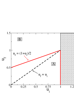
Figure 1: Sketch of the phase diagram in the $u_{i},u_{f}$ plane for the quench dynamics of the single band Hubbard model within the Gutzwiller approximation at half-filling. Two different dynamical regimes corresponding to weak and strong coupling dynamics (A and B in the plot) are found depending whether the final interaction $u_{f}$ lies above or below the critical quench line $u_{fc}=\frac{1+u_{i}}{2}$. For quantum quenches along this line the dynamics features an exponential relaxation toward a steady state.

It is worth noticing that, apart from the trivial case in which $u_{f}=u_{i}$, the classical dynamics (28)-(29) admits a non-trivial stationary solution $D=0$ and $\cos^{2}\phi=u_{f}$, which is compatible with the initial conditions only at half-filling and $u_{f}=u_{fc}=(1+u_{i})/2$. It turns out that $u_{fc}$ identifies a dynamical critical point that separates two different regimes similarly to a simple pendulum. When $u_{f}<u_{fc}$, $2\phi(t)$ oscillates around the origin, while, for $u_{f}>u_{fc}$, it performs a cyclic motion around the whole circle. In order to characterize the different regimes, we focus on three physical quantities, the double occupancy $D(t)$, the quasiparticle residue $Z(t)$ and their period of oscillation, $\mathcal{T}$.

Before discussing in some detail the results of the classical dynamics (28)-(29), it is useful to cast it into a closed first-order differential equation for one of the two conjugate variables $D$ or $\phi$. Indeed the dynamics conserves the energy, namely

$$E(t)=u_{f}D(t)-\frac{\displaystyle n(2-n)}{\displaystyle 8}\,Z(t)\equiv E_{0}\,,\qquad t>0$$ (31)

where $E_{0}$ is the total energy soon after the quench, which reads

$$E_{0}=u_{f}\,D_{i}-\frac{\displaystyle n(2-n)}{\displaystyle 8}\,Z_{i}\,.$$ (32)

with $Z_{i}$ the equilibrium zero temperature quasiparticle weight for interaction $u_{i}$ and doping $\delta$. The simplest way to proceed is to eliminate $\phi$ from Eq.(31) in favor of the double occupancy $D(t)$. From Eq.(III.2) we obtain

$$\cos^{2}\phi=-\frac{E_{0}-u_{f}D+\left(n-2D\right)\left(\sqrt{D+\delta}-\sqrt{D}\right)^{2}/4}{\left(n-2D\right)\sqrt{D\left(D+\delta\right)}},$$ (33)

which can be inserted into (29) and leads, after some algebra, to the equation of motion

$$\dot{D}=\pm\sqrt{\Gamma(D)}\,.$$ (34)

Here $\Gamma(D)$ can be thought as an effective potential controlling the dynamical behavior of $D(t)$. We note that, since the problem is one dimensional, many properties of the solution (34) can be inferred directly from the knowledge of $\Gamma(D)$, without explicitly solving the dynamics. In the next two sections we will discuss in detail the structure of this solution, considering both the half filled and the doped case.

III.3 Quench Dynamics at Half-Filling

We start by considering half-filling, i.e. $\delta=0$, and for simplicity we fix $u_{f}>u_{i}$, see figure 1. As we already anticipated, the dynamical behavior of the system changes drastically when the final value of the interaction $u_{f}$ crosses the critical line $u_{fc}\equiv\left(1+u_{i}\right)/2$.

The existence of such a line of critical values clearly emerges from the structure of the effective potential $\Gamma\left(D\right)$ and in particular from the behavior of its positive roots, which are the inversion points of the one dimensional motion (34).

As one can see from figure 2, $\Gamma(D)$ has three simple zeros, two of them being positive. It turns out that the equilibrium Gutzwiller solution $D_{i}$ is always one of the roots of the effective potential, for any $u_{f}$, see figure 2 (top panels). The remaining two, $D_{\pm}$, depend strongly on $u_{f}$ as we show in the bottom panel of figure 2. Since the one dimensional motion is constrained to the interval $[D_{+},D_{i}]$, where $\Gamma(D)$ is positive, we expect to find periodic solution of the dynamics (34). However, the properties of this solution will largely depend on the behavior of $D_{+}$ as a function of $u_{f}$. As we see, $D_{+}$ first decreases linearly with $u_{f}$, vanishing at $u_{fc}$ where it becomes degenerate with $D_{-}$ (see figure 2). Then for $u_{f}>u_{fc}$ it starts increasing again, approaching $D_{i}$ in the infinite quench limit. It turns out that $D_{+}$ has a simple form, which reads

$$D_{+}=\left\{\begin{array}[]{ll}u_{f}<u_{fc}&\left(u_{fc}-u_{f}\right)/2\\ u_{f}>u_{fc}&D_{i}\left(1-\frac{u_{fc}}{u_{f}}\right)\\ \end{array}\right.$$ (35)

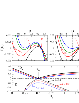
Figure 2: Top Panel: Effective potential $\Gamma\left(D\right)$ for $u_{f}=0.2,0.3,0.4,0.5$ (right) and $u_{f}=0.6,0.8,0.9,1.0$ (left). Bottom panel: Inversion points $D_{+},D_{-}$ as a function of $u_{f}$ at fixed $u_{i}=0$ for zero and finite doping.

Two different dynamical behaviors are therefore expected as a result of this peculiar dependence. In addition, due to the degeneracy of simple roots occurring at $u_{f}=u_{fc}$ we expect here a special trajectory, where relaxation to a steady state can exist. This qualitative picture is confirmed by the actual solution of the classical dynamics (34), whose results we are going to present, both for weak ($u_{f}<u_{fc}$) and strong ($u_{f}>u_{fc}$) quantum quenches.

Weak Quenches: $u_{f}<u_{fc}$

For weak quantum quenches to $u_{f}<u_{fc}$, the dynamics of both double occupation $D(t)$ and quasiparticle weight $Z(t)$ shows coherent oscillations, see figure 3, which do not die out. The lack of relaxation toward a steady state is clearly an artifact of our semiclassical approach that does not account for quantum fluctuations. This is particularly true for weak quenches starting from the gapless metallic phase, where fast damping of the oscillations is expected due to the available continuum of low-lying excitations.

Although oversimplified, the dynamics in the weak quench limit contains some interesting features that are worth to discuss. In particular, we focus on the period $\mathcal{T}$ of the coherent oscillations as a function of the final interaction $u_{f}$. It is easy to see that $\mathcal{T}$ is given by

$$\mathcal{T}=2\,\int_{D_{+}}^{D_{i}}\,\frac{dD}{\sqrt{\Gamma\left(D\right)}}=\frac{4\sqrt{2}\,K\left(k\right)}{\sqrt{Z_{i}}}\,,$$ (36)

where $K\left(k\right)$ is the complete elliptic integral of the first kind with argument $k^{2}=4u_{f}\left(u_{f}-u_{i}\right)/Z_{i}$.

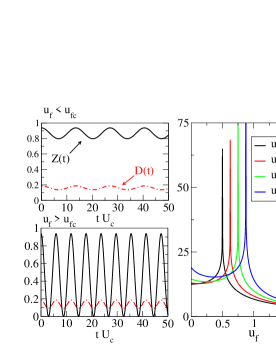
Figure 3: Left Panel: Mean-field dynamics for quantum quenches to $u_{f}$ below (top) and above (bottom) the critical line. Right Panel: Period of oscillation $\mathcal{T}_{D}$ as a function of $u_{f}$ for $u_{i}=0.0,0.25,0.5,0.75$. Notice the log-singularity at $u_{fc}$.

As we show in the right panel of figure 3, upon increasing $u_{f}$ the period $\mathcal{T}$ grows eventually diverging logarithmically as the critical quench line $u_{f}=u_{fc}$ is approached. This can be seen explicitly in Eq.(36). Indeed, for $u_{f}\rightarrow u_{fc}$, the argument of the complete elliptic integral approaches $k=1$

$$1-k^{2}=\left(u_{fc}-u_{f}\right)\left(1+\frac{u_{f}}{2\,u_{fc}\,D_{i}}\right)\,.$$ (37)

Therefore, using the known asymptotic result $K\left(k\right)\simeq\log\left(4/\sqrt{1-k^{2}}\right)$ we find

$$\mathcal{T}\sim\frac{4}{\sqrt{1-u_{i}^{2}}}\,\log\left(\frac{1}{u_{fc}-u_{f}}\right)\,.$$ (38)

Such a diverging time scale signals a sharp transition to a completely different dynamical regime for $u_{f}>u_{fc}$. Before moving to this strong coupling regime we briefly discuss the dynamics of the phase $\phi(t)$ in the weak quench case, which can be easily obtained by eliminating the double occupation $D(t)$ from the original system (28-29). As shown in figure 4, in the present weak quench regime ($u_{f}<u_{fc}$) the phase oscillates around the equilibrium fixed point $\phi=0$, with the same period $\mathcal{T}$. As we are going to discuss in the next paragraph, it is just the phase which shows the most striking change in the dynamics as the critical line is crossed.

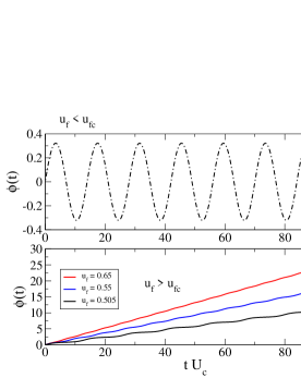
Figure 4: Dynamics of the phase in for quenches below and above the critical value $u_{fc}$. Notice that for small quenches the phase oscillates around zero while for $u_{f}>u_{fc}$ the dynamics is no more bounded since the energy is sufficient to overcome the potential barrier.

Strong Quenches: $u_{f}>u_{fc}$

As we anticipated, for quenches above the critical value $u_{fc}$ the dynamics of the system is qualitatively different, reflecting the change in the behavior of the effective potential inversion points, see equation (35). Let us start discussing the dynamics of double occupancy. Since the effective potential $\Gamma\left(D\right)$ has two simple roots, the motion of double occupation $D(t)$ is still periodic. However, the period $\mathcal{T}$ and the amplitude $\mathcal{A}$ of these strong coupling oscillations decrease upon increasing the strength of the quench, in contrast to the weak quench case. Indeed the latter simply reads $\mathcal{A}=D_{i}-D_{+}\sim 1/u_{f}$ while the period reads

$$\mathcal{T}=\frac{4\,K\left(1/k\right)}{\sqrt{u_{f}\left(u_{f}-u_{i}\right)}}\,,$$ (39)

with argument $1/k$ given by

$$\frac{1}{k}=\sqrt{\frac{2D_{i}\,u_{fc}}{u_{f}\left(u_{f}-u_{i}\right)}}\,.$$ (40)

Deep in the strong coupling regime, $u_{f}\gg\,u_{i}$, we get

$$\mathcal{T}\simeq\,\frac{2\pi}{u_{f}}\,,$$ (41)

smoothly matching the atomic limit result. Hence the resulting dynamics shows very fast oscillations with a reduced amplitude. In the strong quench limit the double occupation dynamics is completely frozen, doublons have no available elastic channel to decay Rosch et al. (2008).

As the critical quench line $u_{fc}$ is approached from above the period of oscillations shows the same logarithmic singularity found on the weak-coupling side. From equation (39) we immediately see that

$$\mathcal{T}\sim\frac{4}{\sqrt{1-u_{i}^{2}}}\,\log\left(\frac{1}{u_{f}-u_{fc}}\right)\,,$$ (42)

namely the same singularity, with the same prefactor, appears on the two side of the dynamical transition.

As already anticipated, it is interesting to discuss the dynamics of the phase $\phi(t)$ when the quench is above the critical line. As shown in figure 4, as soon as the critical line is crossed, the phase starts precessing around the whole circle $(0,2\pi)$. This transition from a localized phase with small oscillations around $\phi=0$ to a delocalized phase where the dynamics is unbounded is, from a mathematical point of view, completely analogous to what happen in a simple pendulum. Right at the critical quench line the dynamics is on the separatrix and the phase takes infinite time to reach its metastable configuration. As we are going to see in the next paragraph this metastable configuration corresponds to a featureless Mott Insulator. Before concluding, let’s briefly discuss the dynamics of quasiparticle weight $Z(t)$ in the strong quench regime. As we see in figure 3, similarly to the double occupation, also $Z(t)$ shows fast oscillations with a period $\mathcal{T}$ given by (41) at strong coupling. Interestingly, the amplitude $\mathcal{A}_{Z}$ of those oscillations goes all the way to zero and keeps finite even for very large $u_{f}$. This can be easily understood by looking at the dependence of the quasiparticle weight from the phase $\phi(t)$. At half filling this simply reads (III.2)

$$Z(t)=16\,D(t)\left(1/2-D(t)\right)\,\cos^{2}\phi(t)\,,$$ (43)

from which we can conclude that, although the double occupation is neither zero nor one half, the quasiparticle weight can vanish due to its phase dependence. As a result of this vanishing minimum we conclude that for $u_{f}\gg 1$, even though the dynamics of double occupancy gets frozen in the initial state, the amplitude of oscillations for $Z$ remains constant and equal to $\mathcal{A}_{Z}=1-u_{i}^{2}$.

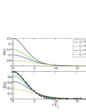
Figure 5: Dynamics after a quench at the critical interaction $u_{fc}$, for different initial conditions $u_{i}$. Both double occupation $D(t)$ and quasiparticle weight $Z(t)$ decay exponentially to zero with a relaxation time $\tau_{\star}\sim 1/\sqrt{Z_{i}}$ which increases with $u_{i}$ approaching the initial Mott Insulator. In the bottom panel we compare the Gutzwiller results with those of DMFT (points, from Ref. Eckstein et al. (2009)) for a quench starting from the non interacting limit.

Critical Line

Quite interestingly, the weak and the strong coupling regimes that we have so far discussed are separated by a critical quench line $u_{fc}$ at which mean-field dynamics exhibits exponential relaxation. This can be seen explicitly since in this limit the effective potential is simply given by $\Gamma\left(D\right)=\,D\sqrt{2u_{fc}\left(D_{i}-D\right)}$, thus the dynamics can be easily integrated to obtain the double occupation $D(t)$ at the critical quench line,

$$D(t)=D_{i}\left(1-\tanh^{2}\left(t/\tau_{\star}\right)\right)\,.$$ (44)

We notice that, independently on the initial value of the correlation $u_{i}$, for $u_{f}=u_{fc}$ the double occupancy relaxes toward zero with a characteristic time scale $\tau_{\star}=4/\sqrt{Z_{i}}$ that increases upon approaching the Mott insulator $u_{i}\rightarrow 1$. Analogously, also the quasiparticle weight $Z(t)$ approaches zero for long-time, with the same exponential behavior,

$$Z(t)=Z_{i}\left(1-\tanh^{2}\left(t/\tau_{\star}\right)\right)\,.$$

Since this is the only case in which our mean field dynamics features a long-time steady state it is worth to compare the above behavior to the DMFT results Eckstein et al. (2009, 2010). In figure 5 we plot the behavior of the quasiparticle residue $Z(t)$ in the two approaches for the case $u_{i}=0$. As we see they both vanishes at long times with a quite good agreement on the time scale. A similar comparison cannot be done for the double occupation $D(t)$ which vanishes at long times in our mean field theory while saturates to a finite small value in DMFT. This is not surprising but again reflects the fact that our mean field dynamics cannot capture the role of incoherent excitations. The long time vanishing of the quasiparticle weight has been interpreted in Refs. Eckstein et al., 2009, 2010 as a signature of thermalization. Although we cannot comment on this issue, since our mean field theory cannot account for thermalization, it is interesting to add some considerations. From our results we see that for quenches at the critical line $u_{fc}$ the system reaches a steady state featuring a complete suppression of charge fluctuations, namely $D=0$ and $Z=0$. This suggests that the above critical line $u_{fc}$ is obtained by tuning the initial energy $E_{0}$ of the quenched correlated metal to the energy of a collection of decoupled half filled sites, the ideal $t_{ij}=0$ Mott insulator. Indeed from this condition we immediately get

$$E_{0}\left(u_{fc},u_{i}\right)=E_{Mott}\longrightarrow u_{fc}=\frac{1+u_{i}}{2}\,.$$ (45)

Surprisingly enough we find that the above condition gives a remarkable good agreement for the dynamical critical point found in DMFT. Indeed if we use that latter criterium, we find an estimate for the critical $U_{fc}$ in units of the hopping integral $t$ and strating from $U_{i}=0$:

$$U_{fc}=4\left|E_{kin}\right|\simeq 3.3\,,$$ (46)

where $E_{kin}$ is the energy of a half-filled Fermi sea with a semielliptic density of states. Eq. (46) is surprisingly close to the result of Refs. Eckstein et al., 2009, 2010.

III.4 Long-time Averages

As we have seen so far, the mean field Gutzwiller dynamics is periodic in the main part of the phase diagram excluding the quench to the critical value $u_{fc}$ where an exponential behavior emerges. In spite of that, it is however worth to investigate a properly defined long-time behavior of the dynamics which, as we are going to show, features many interesting properties. To this extent we firstly introduce, for any given function $O(t)$ an integrated (average) dynamics defined through

$$\langle O\rangle_{t}=\frac{1}{t}\,\int_{0}^{t}\,dt^{\prime}\,O\left(t^{\prime}\right)\,.$$ (47)

Then it is natural to define the long-time average as

$$\bar{O}=\mbox{lim}_{t\rightarrow\infty}\,\langle O\rangle_{t}\,.$$ (48)

Notice that, since the relevant observables are periodic functions of time with period $\mathcal{T}_{O}$ admitting a Fourier decomposition the above definition (48) can be equivalently written as

$$\bar{O}=\frac{1}{\mathcal{T}_{O}}\,\int_{\mathcal{T}_{O}}\,dt\,O(t)\,.$$ (49)

We now study the behavior of steady state averages as a function of the initial and final values of the interaction. We consider the half filled case and for simplicity we assume $u_{f}>u_{i}$. Using equation (49) the average double occupation $\bar{D}$ can be written as which reads

$$\bar{D}=\frac{2}{\mathcal{T}}\,\int_{D_{+}}^{D_{i}}\,\frac{D\,dD}{\sqrt{\Gamma\left(D\right)}}\,,$$ (50)

where $D_{i}$ and $D_{+}$ has been defined in the previous section. In addition, due to energy conservation, the knowledge of the average double occupancy $\bar{D}$ completely fixes the average quasiparticle weight which reads

$$\bar{Z}=Z_{i}+8u_{f}\left(\bar{D}-D_{i}\right)\,.$$ (51)

We now evaluate the long-time average $\bar{D}$ and $\bar{Z}$ as given in Eq. (50-51) in the two different dynamical regimes we have previously identified.

Weak Quenches: $u_{f}<u_{fc}$

In the weak coupling regime and for $u_{f}>u_{i}$ the average double occupation at long times reads

$$\bar{D} = D_{i}\left(1-\frac{u_{fc}}{u_{f}}\right)+D_{i}\frac{u_{fc}}{u_{f}}\,\frac{E\left(k\right)}{K\left(k\right)}=$$ (52)

$$= D_{i}\left[1+\frac{u_{fc}}{u_{f}}\left(\frac{E(k)-K(k)}{K(k)}\right)\right]\,,$$

where $K(k)$ and $E(k)$ are, respectively, the complete elliptic integrals of the first and second kind with argument $k^{2}=\frac{u_{f}\left(u_{f}-u_{i}\right)}{2D_{i}\,u_{fc}}$. Similarly using the Eq. (51) we get for the average quasiparticle weight the result

$$\bar{Z}=Z_{i}\,\frac{E(k)}{K(k)}\,.$$ (53)

It is interesting to consider the asymptotic regime of a small quantum quench $\delta u=u_{f}-u_{i}\rightarrow 0$. Then we can expand the elliptic integrals for small $k$ to get

$$\bar{D}\simeq D_{i}-\frac{\delta u}{4}=\frac{1-u_{f}}{4}\,.$$ (54)

We see therefore that for small quenches the double occupation follows the zero temperature equilibrium curve, independently on the initial value of the interaction $u_{i}$. This is clearly shown in figure 6. Since to lowest order in $\delta u$ no heating effects arise, this result implies that after a small quench of the interaction the average double occupation $\bar{D}$ is thermalized.

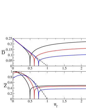
Figure 6: Average double occupation $\bar{D}$ (top) and quasiparticle weight $\bar{Z}$ (bottom) as a function of $u_{f}$ at fixed $u_{i}=0.0,0.25,0.5$ compared to the zero temperature equilibrium result (dashed lines).

In addition, this result has an interesting consequence for what concerns the behavior of the quasiparticle weight $\bar{Z}$. A simple calculation to lowest order in $\delta u$ gives

$$\bar{Z}\simeq Z_{i}-2\,u_{f}\,\left(u_{f}-u_{i}\right)\,,$$ (55)

from which we conclude that, as opposite to the double occupation $\bar{D}$, the long-time average quasiparticle weight differs from the zero temperature equilibrium result even at lowest order in the quench $\delta u$. In particular if we evaluate $\bar{Z}$ for the special case of a quench from a non interacting Fermi Sea ($u_{i}=0$) for which $Z_{i}=1$ we get the result,

$$1-\bar{Z}\left(u_{f}\right)=2\left(1-Z_{eq}\left(u_{f}\right)\right)\,,$$ (56)

firstly obtained in Ref. Moeckel and Kehrein, 2008 within the flow equation approach. This peculiar mismatch between the zero temperature equilibrium quasiparticle residue and its non equilibrium counterpart is a general result of quenching a Fermi Sea Moeckel and Kehrein (2009); Moeckel (2009). It signals the onset of a prethermal regime where quasiparticle are well defined objects, momentum-averaged quantities such as kinetic and potential energy are thermalized while relaxation of distribution functions is delayed to later time scales. We note that our simple mean field theory correctly captures the onset of this long-lived state but fails in describing its subsequent relaxation towards equilibrium.

Interestingly, when approaching the critical quench line from below the average double occupation $\bar{D}$ vanishes logarithmically. Indeed for $k\rightarrow 1$ we have

$$K(k)\simeq\mbox{log}\left(4/\sqrt{1-k^{2}}\right)+O\left(1-k^{2}\right)\,,$$ (57)

and

$$E\left(k\right)\simeq 1+O\left(1-k^{2}\right)\,,$$ (58)

therefore

$$\bar{D}\simeq D_{i}\left(\frac{u_{f}-u_{fc}}{u_{f}}\right)+\frac{2D_{i}}{\mbox{log}\left(\frac{1}{u_{fc}-u_{f}}\right)}\,,$$ (59)

The leading term is therefore logarithmic as mentioned, with linear corrections in $\delta u=u_{fc}-u_{f}$

$$\bar{D}\simeq\frac{2D_{i}}{\mbox{log}\left(\frac{1}{u_{fc}-u_{f}}\right)}\left(1+\frac{\delta u\,\mbox{log}\,\delta u}{2u_{fc}}\right)\,,$$ (60)

A similar behavior is found for the quasiparticle weight $\bar{Z}$ which reads

$$\bar{Z}\simeq\frac{2Z_{i}}{\mbox{log}\left(\frac{1}{u_{fc}-u_{f}}\right)}\,,$$ (61)

Strong Quenches: $u_{f}>u_{fc}$

In the strong coupling regime the average double occupation reads

$$\bar{D}=\frac{u_{fc}-u_{f}}{2}+\frac{u_{f}-u_{i}}{2}\,\frac{E\left(k\right)}{K\left(k\right)}\,,$$ (62)

with the argument given by $k^{2}=\frac{2\,D_{i}\,u_{fc}}{u_{f}\left(u_{f}-u_{i}\right)}$.

Deep in the strong coupling regime, $u_{f}\gg u_{i}$, $k$ goes to zero and we can use the asymptotic for $E(k)$ and $K(k)$

$$\frac{E\left(k\right)}{K\left(k\right)}\simeq 1-\frac{k^{2}}{2}\,,$$ (63)

to obtain

$$\bar{D}\simeq D_{i}\left(1-\frac{u_{fc}}{2u_{f}}\right).$$ (64)

We see therefore that, for infinitely large quenches, $u_{f}\rightarrow\infty$, the dynamics is trapped into the initial state. Interestingly enough, for quenches starting from $u_{i}=0$ the scaling (64) exactly matches the strong coupling perturbative result obtained in Ref. Eckstein et al., 2009 for the prethermal plateau. Indeed using the fact that for $u_{i}=0$ we have $D_{i}\,u_{fc}=1/8=|\bar{\varepsilon}|$, where $\bar{\varepsilon}$ is the kinetic energy of the half-filled Fermi Sea, we find

$$\bar{D}\simeq D_{i}-\frac{|\bar{\varepsilon}|}{2U_{f}}\,,$$

in accordance with strong coupling perturbation theory. The agreement at strong coupling is remarkable if thought from the point of view of thermal equilibrium, where one knows the Gutzwiller wavefunction cannot capture the Hubbard bands, and suggests that our Gutzwiller ansatz can interpolate between the weak and the strong coupling dynamical regime.

As opposite, when approaching the critical quench line from above we obtain a vanishing long-time average, with the same logarithmic behavior we have found on the weak coupling side. Indeed for $u_{f}\rightarrow\,u_{fc}$ from above we have that $k\rightarrow 1^{-}$ and therefore we can again make use of the asymptotic for the complete elliptic integrals. We thus obtain

$$\bar{D}\simeq\frac{2D_{i}}{\mbox{log}\left(\frac{1}{u_{f}-u_{fc}}\right)}\left(1+\frac{\delta u\,\mbox{log}\,\delta u}{4D_{i}}\right)\,.$$ (65)

Note that the approach to zero is the same in both sides of the phase diagram, while the corrections are slightly different.

For what concerns the quasiparticle weight $\bar{Z}$ to get the leading behavior $o\left(1/u_{f}\right)$ we need the double occupancy to next-to-leading order. Expanding the ratio between elliptic functions we get

$$\frac{E\left(k\right)}{K\left(k\right)}\simeq 1-\frac{k^{2}}{2}-\frac{k^{4}}{8}+O\left(k^{6}\right)\,,$$ (66)

and using the expression for $k\simeq Z_{i}/4u_{f}^{2}$ we obtain the following asymptotic behavior for $\bar{Z}$

$$\bar{Z}\simeq Z_{i}-2u_{f}^{2}\,k^{2}\left(1+k^{2}/4\right)\simeq\frac{Z_{i}}{2}\left(1-\frac{Z_{i}}{16u_{f}^{2}}\right)\,,$$ (67)

which shows that also $\bar{Z}$ increases from the critical line to large $u_{f}$ and deep in the strong coupling regime it saturates to a finite plateau which, however does not coincide with its initial value $Z_{i}$ but rather it is smaller by a factor of two due to energy conservation.

III.5 Quench Dynamics away from half-filling

An important outcome of previous sections has been the identification of a critical interaction quench $u_{fc}$ where an exponentially fast relaxation emerges. This value of quenches separates two different dynamical regimes where the system gets trapped into metastable prethermal states. In order to understand the origin of such a sharp transition and its possible relation to equilibrium critical point of the Hubbard model it is natural to extend the mean field analysis away from half-filling, where no transition between a Metal and a Mott Insulator exists in equilibrium. This can be done straightforwardly, for example, by a direct integration of the mean field equations of motion (28-29). It is however more instructive to proceed again by considering the effective dynamics for the double occupation, obtained using the conservation of energy, that we wrote as

$$\dot{D}=\sqrt{\Gamma(D)}\,,$$ (68)

We now argue that any finite doping $\delta$ is enough to wash out the dynamical critical point and turn it into a crossover. To see this, it is worth to consider again the effective potential $\Gamma\left(D\right)$ which enters the above dynamics. Indeed the qualitative analysis we have performed in section III.3 can be done even for finite doping $\delta$. As we will show explicitly in the Appendix A the effective potential keep the same structure for $\delta\neq 0$, with three inversion points respectively given by $D_{i}$ - the zero temperature finite doping Gutzwiller solution - and $D_{\pm}$.

Figure 7: Top Panel: amplitude $\mathcal{A}_{D}$ (left) and period $\mathcal{T}_{D}$ at $u_{i}=0$ and $\delta=0.0,0.05,0.10,0.20,0.30$. Bottom Panel: averages double occupancy $\bar{D}$ (left) and quasiparticle weight $\bar{Z}$ (right) at $u_{i}=0$ and $\delta=0.0,0.05,0.10,0.20,0.30$.

As a consequence, all the differences between the doped and the half-filled case are hidden in the behavior of the two non-trivial roots $D_{+},D_{-}$ as a function of $u_{f}$. Their explicit expression is quite lengthy and it is reported for completeness in Appendix A. As we can see from figure 2, those two roots, which at half-filling are degenerate at $u_{fc}$, are always distinct at finite doping. In particular at the half-filling critical quench line $u_{fc}$, we find at finite doping

$$D_{+}(u_{fc})-D_{-}(u_{fc})\simeq\delta\,.$$

As a consequence the dynamics of double occupancy (and hence of quasiparticle weight) always features a finite period given by

$$\mathcal{T}\simeq\frac{K\left(k\right)}{\sqrt{u_{f}\left(D_{i}-D_{-}\right)}}\,,$$ (69)

with the argument $k$ of the elliptic function defined in term of the inversion points as

$$k=\sqrt{\left(D_{i}-D_{+}\right)/\left(D_{i}-D_{-}\right)}\,.$$ (70)

Notice that, since the two inversion points never collapse $D_{+}>D_{-}$, the argument $k$ is always strictly lesser than one, $k<1$, and no singularity in $\mathcal{T}$ arises.

In figure 7 (top panels) we plot the period $\mathcal{T}$ and the amplitude $\mathcal{A}$ of the double occupancy oscillations in the doped case, as a function of $u_{f}$ at fixed $u_{i}$. We notice that both quantities are smooth across $u_{fc}$, and in particular the logarithmic singularity in the period turns into a sharp peak which broadens out as the doping increases.

We finally remark that a small doping not only affects the dynamics, but also drastically changes the long-time averages properties with respect to the results we have depicted in section III.3. This can be worked out explicitly by using the same equations we have obtained for the half-filling case, cfr. section III.4, provided the correct expression for the roots $D_{+},D_{-}$ is used. As we can see from figure 7 both double occupation and quasiparticle weight stay always finite as $u_{f}$ increases and only show a dip around the critical quench line which is gradually smoothed out as the doping increases.

In conclusion, we have shown that the dynamical transition described in section III.3 is a peculiar feature of the half-filled case, namely that any finite doping $\delta\neq 0$ is enough to wash out this dynamical transition, cutting off the logarithmic divergence in the oscillation period $\mathcal{T}$.

III.6 Discussion

We conclude this section by discussing the results of our time dependent mean field theory for the fermionic Hubbard model in light of those recently obtained in the literature using different approaches, such as the Flow Equation method  Moeckel and Kehrein (2008, 2009) and the Non Equilibrium Dynamical Mean Field Theory Eckstein et al. (2009, 2010), both of which considered a quantum quench starting from an half-filled non interacting Fermi Sea. As we already mentioned, our mean field results feature an oversimplified periodical dynamics that lacks relaxation to a steady state at long times. This can be traced back to the suppression of quantum fluctuations which is at the ground of our treatment. In this respect we notice that both approaches work much better, displayng some damping at long times. Beside this obvious drawback we can say that, quite remarkably, a mean field theory catches many interesting features of the problem.

First of all our variational ansatz is able to capture both regimes of pre-thermalization found at weak Moeckel and Kehrein (2008) and strong coupling Eckstein et al. (2009). Those long lived metastable regimes, which are, respectively, due to Fermi statistics and to long-lived double occupations, are quantitatively reproduced by our approach as it appears clearly from the analysis of long time averages (see Eqs. (55) and (64)). However, as generally expected in mean field theories, those metastable states are wrongly predicted to have infinite lifetime. A second interesting point that clearly emerges from our analysis is the existence of a dynamical critical line that separates those two distinct regimes, and where an exponentially fast relaxation emerges, as firstly shown in Ref. Eckstein et al., 2009. On one hand, the existence of a dynamical critical point could be anticipated since at equilibrium the model undergoes a quantum phase transition, the Mott transition. Indeed, as we have shown, any finite doping turns the dynamical transition into a crossover. On the other hand, it was noted in Ref. Eckstein et al., 2009 that the energy pumped in the quench at $U_{fc}$ with $U_{i}=0$ would correspond, should thermalization be assumed, to an effective temperature $T_{\star}$ higher than the Mott ending point, where no critical dynamics could have been foreseen. Such an observation points to a dynamical transition that could be associated with loss of ergodicity and which is not incompatible with our finding that the critical quench occurs when the correlated metal is initially prepared with the energy of the ideal Mott insulator, a collection of independent sites. Interestingly enough, such a condition gives a excellent match with the DMFT estimate of the dynamical critical point (see equation 46). Finally, we note that the issue of a non equilibrium dynamical transition in the quench dynamics of interacting quantum systems seems to be of more general interest. Indeed recent investigations on the fully connected Bose Hubbard model Sciolla and Biroli (2010) and the scalar $\phi^{4}$ mean field theory  Gambassi and Calabrese (2010) reveals that a very similar phenomenon is present in these models as well. Whether this is an artifact of the mean field approximation or rather a generic feature of the quench dynamics of interacting quantum systems in more than one dimension, as recent works would suggest, Gambassi and Calabrese (2010) is an interesting subject that requires further investigations. In this respect an interesting question is the role played by small quantum fluctuations on such a dynamical transition. We will try to partially address this issue in the remaining part of this paper.

IV $Z_{2}$ Slave Spin Formulation

We have shown that, within the Gutzwiller approximation, the variational principle when applied to the Shrœdinger equation amounts to determine the saddle point of an action $S\left[\phi_{i\alpha},O_{i\alpha},\Phi\right]$ that depends on pairs of conjugate fields, $\phi_{i\alpha}$ and $O_{i\alpha}$, and on a Slater determinant or BCS wavefunction. The saddle point reduces to a set of first order coupled differential equations for the conjugate fields and for the average values of single particle operators on $|\Phi(t)\rangle$. One could be tempted to interpret this result as the mean field decoupling of the Heisenberg equations of motion for the average values of a set of quantum operators corresponding to some effective quantum Hamiltonian. Identifying such a quantum Hamiltonian could then allow adding quantum fluctuations on top of the mean field results. This is right the same conceptual scheme invoked to associate the time-dependent Hartree-Fock equations to an effective Hamiltonian of non-interacting bosons that represent particle-hole excitations. In our case we would expect the quantum Hamiltonian to describe free electrons coupled to a set of conjugate Bose fields, $\phi_{i\alpha}$ and $O_{i\alpha}$, which in fact resembles the conventional slave-boson approaches to correlated systems.

We are going to show that this program can be easily accomplished in the simple Hubbard model, although in a different and more rigorous manner than simply quantizing the classical equations of motion. To this extent we formulate the original Hubbard model in terms of an auxiliary Quantum Ising Model in a transverse field coupled to free fermionic quasiparticles, in the framework of the recently introduced $Z_{2}$ slave spin theory Huber and Rüegg (2009); Rüegg et al. (2010).

IV.1 Mapping onto a Quantum Ising Model in a Transverse Field

The idea of writing the Hubbard model in terms of auxiliary spins coupled to free quasiparticles is not new.de’Medici et al. (2005); Hassan and de’ Medici (2010) A minimal formulation in terms of a single Ising spin and a fermionic degrees of freedom has been recently introduced,Huber and Rüegg (2009); Rüegg et al. (2010) based on a mapping between the local physical Hilbert space of the Hubbard Model and the Hilbert space of the auxiliary model subjected to a constraint. Here we derive the same mapping by showing that the identification holds for the partition functions as well, when evaluated order by order in perturbation theory in $U$. The advantage of this alternative formulation is that the role of the lattice coordination emerges more clearly.

We write the Hubbard interaction as

$$U\,n_{\uparrow}\,n_{\downarrow}=\frac{U}{4}\,\Big{[}2(n-1)^{2}-1\Big{]}+\frac{U}{4}\,(2n-1).$$

The last term can be absorbed into the chemical potential, so that we shall consider as interaction only the first term. We define

$$2(n-1)^{2}-1=\mathrm{e}^{i\pi\,n}\equiv\Omega,$$ (71)

where the operator $\Omega$ is real and unitary and has eigenvalues $-1$ for $n=1$ and $+1$ for $n=0,2$. It follows that

$$\Omega\,c^{\dagger}_{\sigma}\,\Omega=-c^{\dagger}_{\sigma},$$ (72)

namely it changes sign to the fermion operator.

Let us concentrate on a given site, with local energy $\epsilon$, whose Fermi operator we shall denote as $c^{\dagger}_{\sigma}$ and density operator $n$. The rest of the lattice sites, Fermi operators $d_{\mathbf{R}\sigma}$, are described by the generically interacting Hamiltonian $H_{bath}$ and are coupled to the site under investigation by

$$H_{tunn}=-\sum_{\mathbf{R}\sigma}\,t_{\mathbf{R}}\,c^{\dagger}_{\sigma}d^{\phantom{\dagger}}_{\mathbf{R}\sigma}+H.c..$$ (73)

We shall denote as

$$H_{0}=H_{bath}+\epsilon\,n+H_{tunn},$$

the unperturbed Hamiltonian and

$$\frac{\displaystyle U}{\displaystyle 4}\,\mathrm{e}^{i\pi\,n}=\frac{\displaystyle U}{\displaystyle 4}\,\Omega,$$

the perturbation. Suppose we calculate the partition function within perturbation theory. A generic $n$-th order correction to the partition function is

$$Z^{(n)} = \left(-\frac{\displaystyle U}{\displaystyle 4}\right)^{n}\,\int_{0}^{\beta}\,d\tau_{1}\,\int_{0}^{\tau_{1}}\,d\tau_{2}\,\dots\int_{0}^{\tau_{n-1}}\,d\tau_{n}\,\mathrm{Tr}\Bigg{[}\mathrm{e}^{-\left(\beta-\tau_{1}\right)\,H_{0}}\,\Omega\,\mathrm{e}^{-\left(\tau_{1}-\tau_{2}\right)\,H_{0}}\,\Omega\,\dots\,\Omega\,\mathrm{e}^{-\left(\tau_{n-1}-\tau_{n}\right)\,H_{0}}\,\Omega\,\mathrm{e}^{-\left(\tau_{n}-0\right)\,H_{0}}\Bigg{]}\,,$$

Because of (72) $\Omega\,H_{0}\,\Omega=H_{bath}+\epsilon\,n-H_{tunn}\equiv H_{1}$. We shall distinguish the two cases of $n$ even or odd. In the even case one easily realizes that

$$Z^{(2n)} = \left(\frac{\displaystyle U}{\displaystyle 4}\right)^{2n}\,\int_{0}^{\beta}\,d\tau_{1}\,\int_{0}^{\tau_{1}}\,d\tau_{2}\,\dots\int_{0}^{\tau_{2n-1}}\,d\tau_{2n}\,$$ (74)

$$~{}~{}~{}~{}~{}~{}~{}~{}\mathrm{Tr}\Bigg{[}\mathrm{e}^{-\left(\beta-\tau_{1}\right)\,H_{0}}\,\mathrm{e}^{-\left(\tau_{1}-\tau_{2}\right)\,H_{1}}\,\mathrm{e}^{-\left(\tau_{2}-\tau_{3}\right)\,H_{0}}\,\dots\,\mathrm{e}^{-\left(\tau_{2n-1}-\tau_{2n}\right)\,H_{1}}\,\mathrm{e}^{-\left(\tau_{2n}-0\right)\,H_{0}}\Bigg{]},$$

which resembles an iterated X-ray edge problem, like in the Anderson-Yuval representation of the Kondo model. We note that, since $\Omega^{2}=1$, Eq. (74) is invariant under $H_{0}\leftrightarrow H_{1}$. For the odd case, one finds instead

$$Z^{(2n+1)}=-\left(\frac{\displaystyle U}{\displaystyle 4}\right)^{2n+1}\,\int_{0}^{\beta}\,d\tau_{1}\,\int_{0}^{\tau_{1}}\,d\tau_{2}\,\dots\int_{0}^{\tau_{2n}}\,d\tau_{2n+1}\,$$

$$\mathrm{Tr}\Bigg{[}\mathrm{e}^{-\left(\beta-\tau_{1}\right)\,H_{0}}\,\mathrm{e}^{-\left(\tau_{1}-\tau_{2}\right)\,H_{1}}\,\mathrm{e}^{-\left(\tau_{2}-\tau_{3}\right)\,H_{0}}\,\dots\,\mathrm{e}^{-\left(\tau_{2n-1}-\tau_{2n}\right)\,H_{1}}\,\mathrm{e}^{-\left(\tau_{2n}-\tau_{2n+1}\right)\,H_{0}}\,\mathrm{e}^{-\left(\tau_{2n+1}-0\right)\,H_{1}}\,\Omega\Bigg{]}.$$

(75)

Once again the above expression is also equal to that one where $H_{0}$ is interchanged with $H_{1}$.

Can one reproduce the same perturbative expansion with some other model? Let us consider an Ising-like Hamiltonian $H_{Ising}=H_{*}+H_{transv}$ where the unperturbed term is

$$H_{*}=H_{bath}+\epsilon\,n+\sigma^{x}\,H_{tunn},$$ (76)

the perturbation is

$$H_{transv}=-\frac{\displaystyle U}{\displaystyle 4}\,\sigma^{z},$$ (77)

and $\sigma^{a}$, $a=x,y,z$, are Pauli matrices. If we take the trace over eigenstates of $\sigma^{x}$ – note that for $\sigma^{x}=1$ $H_{*}=H_{0}$, while for $\sigma^{x}=-1$ $H_{*}=H_{1}$ – the perturbation (77) may act only an even number of times and one easily find that the final result is just twice (74). In other words, $Z^{(2n)}$ is half of the $2n$-th order term in the perturbative expansion of the Ising model $H_{Ising}$. How do we get the odd order terms in the expansion? Let us consider the perturbative expansion of

$$-\mathrm{Tr}\Bigg{(}\mathrm{e}^{-\beta\,H_{Ising}}\,\sigma^{z}\,\Omega\Bigg{)}.$$

It is clear that now only odd terms in the expansion over eigenstates of $\sigma^{x}$ will contribute and one easily realizes that the final result is twice (75).

Therefore, the partition function of the original model is also equal to

$$Z=\mathrm{Tr}\Bigg{[}\mathrm{e}^{-\beta\,H_{Ising}}\,\left(\frac{\displaystyle 1-\sigma^{z}\,\Omega}{\displaystyle 2}\right)\Bigg{]}.$$ (78)

We note that

$$\mathcal{Q}=\frac{\displaystyle 1-\sigma^{z}\,\Omega}{\displaystyle 2},$$ (79)

is actually a projector of the enlarged Hilbert space onto the subspace where if $n=1$ then $\sigma^{z}=+1$ while, if $n=0,2$, then $\sigma^{z}=-1$. As a matter of fact, $\mathcal{Q}$ is just the constraint introduced in Ref. Rüegg et al., 2010 as a basis of the $Z2$ slave-spin representation of the Hubbard model. In fact, what we have done here is simply re-deriving the mapping of Ref. Rüegg et al., 2010 in a different way. There are however some interesting aspects of the mapping that emerge clearly at the level of the partition functions and were not discussed in Ref. Rüegg et al., 2010.

We note that what we have shown so far is that, given an Anderson impurity model with Hamiltonian

$$H_{AIM} = H_{bath}+H_{tunn}+\epsilon\,n+\frac{U}{2}\,(n-1)^{2}$$ (80)

$$= H_{bath}+H_{tunn}+\epsilon\,n+\frac{U}{4}\,\left(1+\Omega\right),$$

its partition function can be also written as

$$Z_{AIM} = \frac{1}{2}\,\mathrm{Tr}\Bigg{[}\mathrm{e}^{-\beta\,H_{Ising}}\,\bigg{(}1-\sigma^{z}\,\Omega\bigg{)}\Bigg{]}$$ (81)

$$= \frac{1}{2}\,Z_{Ising}\,\bigg{(}1-\langle\sigma^{z}\,\Omega\rangle\bigg{)},$$

where

$$H_{Ising}=H_{bath}+\epsilon\,n+\sigma^{x}\,H_{tunn}+\frac{U}{4}\,\left(1-\sigma^{z}\right),$$ (82)

and

$$Z_{Ising}=\mathrm{Tr}\left(\mathrm{e}^{-\beta H_{Ising}}\right).$$

As mentioned above, $Z_{Ising}$ is even in $U$, while $\langle\sigma^{z}\,\Omega\rangle$ is odd. As a simple byproduct, we note that, if particle-hole symmetry holds, the partition function must be even in $U$, so that

$$Z_{AIM}\equiv\frac{1}{2}\,Z_{Ising},$$ (83)

hence the constraint is uneffective and the mapping holds trivially. It was noticed in Ref. Rüegg et al., 2010 that $H_{Ising}$ in (82) possesses a local $Z_{2}$ gauge symmetry, $c^{\dagger}_{\sigma}\to-c^{\dagger}_{\sigma}$ and $\sigma^{x}\to-\sigma^{x}$, which can not be broken. Indeed, the factor $1/2$ in (83) avoids the consequent double counting.

One can straightforwardly extend the above procedure to a collection of interacting sites, hence to the Hubbard model, with the final result that

$$Z=\mathrm{Tr}\Bigg{[}\mathcal{Q}\;\mathrm{e}^{-\beta\,H_{Ising}}\Bigg{]},$$ (84)

where now

$$H_{Ising}=-t\sum_{<\mathbf{R},\mathbf{R^{\prime}}>\,\sigma}\,\sigma^{x}_{\mathbf{R}}\,\sigma^{x}_{\mathbf{R^{\prime}}}\,c^{\dagger}_{\mathbf{R}\sigma}c^{\phantom{\dagger}}_{\mathbf{R^{\prime}}\sigma}+\frac{U}{4}\sum_{\mathbf{R}}\,\left(1-\sigma^{z}_{\mathbf{R}}\right).$$ (85)

and the constraint is

$$\mathcal{Q}=\prod_{\mathbf{R}}\left(\frac{\displaystyle 1-\sigma^{z}_{\mathbf{R}}\Omega_{\mathbf{R}}}{\displaystyle 2}\right).$$ (86)

We note that, if $\tau\to-it$, the mapping still holds and shows that the time-evolution of the Hubbard model can be mapped onto the time evolution of $H_{Ising}$. In particular, since $\left[\mathcal{Q},H_{Ising}\right]=0$, the two evolutions are exactly the same on a state that satisfies the constraint.

IV.2 Recovering the Gutzwiller approximation at equilibrium

Let us now consider a lattice whose coordination tends to infinity in a such a way that the hopping energy per site remains well defined. In this limit, it is well knownGeorges et al. (1996) that the Hubbard model maps onto an Anderson impurity model self-consistently coupled to a conduction bath. We showed earlier that when particle-hole symmetry holds, the constraint is uneffective for the mapping of the Anderson impurity model to the Ising model. It follows that the same holds also for the Hubbard model, in which case

$$Z_{Hubbard}=\left(\frac{1}{2}\right)^{N}\,Z_{Ising},$$ (87)

where $N$ is the number of sites.

Therefore, in infinite coordination lattices and at particle-hole symmetry, we could calculate the partition function of the model

$$H_{Ising}=-\frac{\displaystyle t}{\displaystyle\sqrt{z}}\sum_{<\mathbf{R},\mathbf{R^{\prime}}>\,\sigma}\,\sigma^{x}_{\mathbf{R}}\,\sigma^{x}_{\mathbf{R^{\prime}}}\,c^{\dagger}_{\mathbf{R}\sigma}c^{\phantom{\dagger}}_{\mathbf{R^{\prime}}\sigma}+\frac{U}{4}\sum_{\mathbf{R}}\,\left(1-\sigma^{z}_{\mathbf{R}}\right),$$ (88)

and obtain that of the Hubbard model through (87). The factor $z$ in (88) is the lattice coordination and must be sent to infinity at the end of the calculation.Georges et al. (1996) It turns out that the Gutzwiller approximation is nothing but the mean field decoupling of $H_{Ising}$, assuming a wavefunction product of an Ising part times a fermionic one. The degeneracy of the solution that derives from the local $Z_{2}$ gauge symmetry, $\sigma^{x}_{\mathbf{R}}\to-\sigma^{x}_{\mathbf{R}}$ and $c^{\dagger}_{\mathbf{R}\sigma}\to-c^{\dagger}_{\mathbf{R}\sigma}$ is canceled out by the $(1/2)^{N}$ factor in (87).

To recover the Gutzwiller result for the Mott transition, let us consider a trial translationally-invariant wavefunction $|\Psi\rangle=|\Phi_{\sigma}\rangle\,|\Phi_{c}\rangle$, where $|\Phi_{\sigma}\rangle$ is a Ising-spin state and $|\Phi_{c}\rangle$ an electron one. If we define

$$-t\frac{\displaystyle 1}{\displaystyle\sqrt{z}}\,\sum_{\sigma}\,\langle\Phi_{c}|\,c^{\dagger}_{\mathbf{R}\sigma}c^{\phantom{\dagger}}_{\mathbf{R^{\prime}}\sigma}+H.c.\,|\Phi_{c}\rangle=-\frac{2}{z}\,\varepsilon,$$

where $-\varepsilon$ is the average hopping energy per site of $|\Phi_{c}\rangle$, then the average value per site of the Hamiltonian (88) is

$$E=\langle\Phi_{\sigma}|\,-\varepsilon\,\frac{\displaystyle 2}{\displaystyle z}\sum_{<\mathbf{R},\mathbf{R^{\prime}}>}\sigma^{x}_{\mathbf{R}}\,\sigma^{x}_{\mathbf{R^{\prime}}}+\frac{U}{4}\sum_{\mathbf{R}}\left(1-\sigma^{z}_{\mathbf{R}}\right)\,|\Phi_{\sigma}\rangle,$$

i.e. the energy of an Ising model in a transverse field. We assume $|\Phi_{\sigma}\rangle=\mathcal{U}\,|\Phi_{0}\rangle$ where the unitary operator

$$\mathcal{U}=\exp\left(i\frac{\beta}{2}\sum_{\mathbf{R}}\,\sigma^{y}_{\mathbf{R}}\right),$$ (89)

so that $E$ becomes the average value on $|\Phi_{0}\rangle$ of the Hamiltonian

$$H_{*} = \frac{U}{4}\sum_{\mathbf{R}}\,1-\cos\beta\,\sigma^{z}_{\mathbf{R}}-\sin\beta\,\sigma^{x}_{\mathbf{R}}$$ (90)

$$-\varepsilon\,\frac{2}{z}\sum_{<\mathbf{R},\mathbf{R^{\prime}}>}\,\Big{(}\cos\beta\,\sigma^{x}_{\mathbf{R}}-\sin\beta\,\sigma^{z}_{\mathbf{R^{\prime}}}\Big{)}$$

$$\phantom{-\varepsilon\,\frac{2}{z}\sum_{<i,j>}}\;\Big{(}\cos\beta\,\sigma^{x}_{\mathbf{R^{\prime}}}-\sin\beta\,\sigma^{z}_{\mathbf{R^{\prime}}}\Big{)}.$$

We assume that $|\Phi_{0}\rangle$ is so close to the fully ferromagnetic state with all spins oriented along $x$ that we can set

$$\sigma^{x}_{\mathbf{R}} \simeq 1-\left(x_{\mathbf{R}}^{2}+p_{\mathbf{R}}^{2}-1\right)\equiv 1-\Pi_{\mathbf{R}},$$ (91)

$$\sigma^{y}_{\mathbf{R}} \simeq -\sqrt{2}\,p_{\mathbf{R}},$$ (92)

$$\sigma^{z}_{\mathbf{R}} \simeq \sqrt{2}\,x_{\mathbf{R}},$$ (93)

where $x_{\mathbf{R}}$ and $p_{\mathbf{R}}$ are conjugate variables. If we substitute the above expressions in (90) and fix $\beta$ in such a way that all terms linear in $x_{\mathbf{R}}$ vanish, we find

$$\sin\beta=\frac{\displaystyle U}{\displaystyle 8\varepsilon},$$ (94)

for $U<8\varepsilon\equiv U_{c}$, while $\sin\beta=1$ otherwise. $U_{c}$ is the mean-field value of critical transverse field that separates the ordered phase from the disordered one in the Ising model. It also identifies the Mott transition in the original Hubbard model, and, in fact, the value of $U_{c}$ coincides with that of the Gutzwiller approximation. Because of the above choice of $\beta$, once we expand the Hamiltonian (90) up to second order in $x_{\mathbf{R}}$ and $p_{\mathbf{R}}$ we find, apart from constant terms and in units of $U_{c}$,

$$H_{*}\simeq\frac{a}{2}\sum_{i}\Big{(}x_{\mathbf{R}}^{2}+p_{\mathbf{R}}^{2}\Big{)}-\frac{b}{2}\,\frac{2}{z}\sum_{<\mathbf{R},\mathbf{R^{\prime}}>}\,x_{\mathbf{R}}\,x_{\mathbf{R^{\prime}}},$$ (95)

where $a=1/2$ and $b=u^{2}/2$ for $u=(U/U_{c})<1$, the metallic phase, while $a=u/2$ and $b=1/2$ for $u>1$, the Mott insulator. The spectrum of the excitations on both side of the transition is that of acoustic modes with dispersion in momentum space

$$\omega_{\mathbf{q}}=\sqrt{a\left(a-b\gamma_{\mathbf{q}}\right)},$$ (96)

where, assuming a hypercubic lattice in $d=z/2$ dimensions,

$$\gamma_{\mathbf{q}}=\frac{1}{d}\sum_{a=1}^{d}\,\cos q_{a}\in[-1,1],$$ (97)

with $q_{a}$ the components of the wavevector $\mathbf{q}$. At the transition $a=b$ and the spectrum becomes gapless at ${\mathbf{q}}=0$. In principle, at the same level of approximation one should also take into account the coupling between the spin-waves of the Ising model and the conduction electrons via the hopping term in (88). We just mention that, deep in the insulating side, where $\omega_{\mathbf{q}}\sim u/2\gg 1$, one can integrate out the acoustic modes and obtain the antiferromagnetic Heisenberg model known to be the large $U$ limit of the half-filled Hubbard model. A thorough analysis of the role of quantum fluctuations at equilibrium has been presented in Ref. Rüegg et al., 2010 in connection with the $Z_{2}$-slave-spin theory for correlated fermions, to which we refer for further details. In what follows, we shall instead discuss a way to add quantum fluctuations in an out-of-equilibrium situation.

IV.3 Recovering the Gutzwiller approximation out-of-equilibrium

Because the two models can be mapped onto each other, a quantum quench in the Hubbard model is equivalent to suddenly change the transverse field in the Ising-like model (88) at particle-hole symmetry and in the limit of infinite coordination lattices. We shall keep assuming a factorized time-dependent trial wavefunction $|\Phi_{\sigma}(t)\rangle\,|\Phi_{c}(t)\rangle$, each component $|\Phi_{\sigma}(t)\rangle$ and $|\Phi_{c}(t)\rangle$ being translationally invariant. The electron wavefunction will evolve under the action of a time-dependent hopping, which is however still translationally invariant. Hence, if $|\Phi_{c}(t=0)\rangle$ is eigenstate of the hopping at $t<0$, in particular its ground state state, it will stay unchanged under the time evolution. Therefore we shall only focus on the evolution of the Ising component. Its Hamiltonian at positive times and in units of $U_{c}$ is

$$H=-\frac{u_{f}}{4}\sum_{\mathbf{R}}\,\Big{(}1-\sigma^{z}_{\mathbf{R}}\Big{)}-\frac{1}{8}\,\frac{2}{z}\sum_{<\mathbf{R}\,\mathbf{R^{\prime}}>}\,\sigma^{x}_{\mathbf{R}}\,\sigma^{x}_{\mathbf{R^{\prime}}},$$ (98)

and we assume that at time $t=0$ $|\Phi_{\sigma}(t=0)\rangle$ is the approximate ground state defined in the previous section IV.2 for a different transverse field $u_{i}$. The time-evolution is thus described by the Schrœdinger equation

$$i\partial_{t}\,|\Phi_{\sigma}(t)\rangle=H\,|\Phi_{\sigma}(t)\rangle.$$ (99)

We assume

$$|\Phi_{\sigma}(t)\rangle=\mathcal{U}(t)\,|\Phi_{0}(t)\rangle,$$ (100)

where now

$$\mathcal{U}(t)=\exp\left(i\frac{\alpha(t)}{2}\sum_{i}\,\sigma^{x}_{\mathbf{R}}\right)\,\exp\left(i\frac{\beta(t)}{2}\sum_{\mathbf{R}}\,\sigma^{y}_{\mathbf{R}}\right).$$ (101)

It follows that $|\Phi_{0}\rangle$ must satisfy the equation of motion

$$i\partial_{t}\,|\Phi_{0}(t)\rangle=H_{*}(t)\,|\Phi_{0}(t)\rangle,$$ (102)

where, apart from constants,

$$H_{*}(t) = -i\,\mathcal{U}(t)^{\dagger}\,\dot{\mathcal{U}}(t)+\mathcal{U}(t)^{\dagger}\,H\,\mathcal{U}(t)$$

$$= \sum_{\mathbf{R}}\,\Bigg{[}\frac{\displaystyle\dot{\alpha}}{\displaystyle 2}\,\cos\beta\,\sigma^{x}_{\mathbf{R}}-\frac{\displaystyle\dot{\alpha}}{\displaystyle 2}\,\sin\beta\,\sigma^{z}_{\mathbf{R}}+\frac{\displaystyle\dot{\beta}}{\displaystyle 2}\,\sigma^{y}_{\mathbf{R}}$$

$$-\frac{\displaystyle u_{f}}{\displaystyle 4}\bigg{(}\cos\alpha\,\cos\beta\,\sigma^{z}_{\mathbf{R}}+\cos\alpha\,\sin\beta\,\sigma^{x}_{\mathbf{R}}$$

$$~{}~{}~{}~{}~{}~{}~{}~{}~{}~{}~{}~{}~{}~{}~{}~{}~{}~{}~{}~{}-\sin\alpha\,\sigma^{y}_{\mathbf{R}}\bigg{)}\Bigg{]}$$

$$-\frac{1}{8}\,\frac{2}{z}\sum_{<\mathbf{R},\mathbf{R^{\prime}}>}\,\Big{(}\cos\beta\,\sigma^{x}_{\mathbf{R}}-\sin\beta\,\sigma^{z}_{\mathbf{R}}\Big{)}$$

$$\phantom{-\frac{1}{8}\,\frac{2}{z}\sum_{<i,j>}}\;\;\;\Big{(}\cos\beta\,\sigma^{x}_{\mathbf{R^{\prime}}}-\sin\beta\,\sigma^{z}_{\mathbf{R^{\prime}}}\Big{)}.$$

In the same spirit of the spin-wave approximation above, we shall assume that $|\Phi_{0}(t)\rangle$ is at any time close to a fully polarized state along $x$, so that we can safely use the approximate expressions (91)–(93) for the spin operators. Just like before, we fix $\alpha(t)$ and $\beta(t)$ in such a way that all linear terms in $x_{\mathbf{R}}$ and $p_{\mathbf{R}}$ vanish and find the following set of equations

$$\dot{\beta} = -\frac{u_{f}}{2}\,\sin\alpha,$$ (104)

$$\dot{\alpha} = \frac{1}{2}\,\cos\beta-\frac{u_{f}}{2}\,\cos\alpha\,\cot\beta.$$ (105)

These equations have to be solved starting from the initial condition appropriate to the approximate ground state with transverse field $u_{i}$, i.e. $\alpha(0)=0$ and $\sin\beta(0)=u_{i}$ if $u_{i}<1$ otherwise $\sin\beta(0)=1$, see Eq. (94). In addition, as noticed before, the equations admit a constant of motion, which can be regarded as the classical energy,

$$E=-\frac{u_{f}}{4}\,\cos\alpha\,\sin\beta-\frac{1}{8}\,\cos^{2}\beta.$$

One can readily recognize that the dynamical system (104)–(105) is equivalent to that one we previously obtained within the time-dependent Gutzwiller approximation. However, as we are going to see in the next section, this alternative formulation however allows us to access quantum fluctuations, assuming they are small.

IV.4 Quantum Fluctuations beyond mean field dynamics

The time dependent hamiltonian $H_{\star}(t)$ we have obtained in the previous section, Eq (IV.3), accounts in principle for quantum fluctuation effects. A simple way to proceed is to fix the parameters $\alpha(t)$ and $\beta(t)$ in such a way Eqs. (104) and (105) are satisfied, and expand the hamiltonian up to second order in $x_{\mathbf{R}}$ and $p_{\mathbf{R}}$. The result has no more linear terms and simply describes coupled harmonic oscillators with time-dependent parameters.

$$H_{*}(t) \simeq \frac{\displaystyle u_{f}\cos\alpha(t)}{\displaystyle 4\sin\beta(t)}\,\sum_{\mathbf{R}}\Big{(}x_{\mathbf{R}}^{2}+p_{\mathbf{R}}^{2}\Big{)}$$ (106)

$$-\frac{\displaystyle\sin^{2}\beta(t)}{\displaystyle 4}\,\frac{2}{z}\,\sum_{<\mathbf{R},\mathbf{R^{\prime}}>}\,x_{\mathbf{R}}\,x_{\mathbf{R^{\prime}}},\,$$

We note that such a treatment, similar to what we have done in equilibrium, is equivalent to include gaussian fluctuations without renormalizing the transition point. In other words, we are studying the effect of quantum fluctuations around the semiclassical trajectory without allowing any feedback of these on the latter, which could be dangerous, as we shall see. We shall analyze the time dependent problem (106) separately in the two different cases of quenching from the correlated metal or from the Mott insulator, starting from the latter that is simpler.

IV.4.1 Quenching from the Mott insulator

In this case $u_{i}>1$ and the initial values of the Euler angles are $\alpha(0)=0$ and $\sin\beta(0)=1$. It follows from Eqs. (105) and (104) that these angles will not evolve in time so that $H_{*}$ in (106) does not depend on time and coincides with (95) for $a=u_{f}/2$ and $b=1/2$. This Hamiltonian is well defined provided $u_{f}>1$, which simply reflects that our assumption of weak quantum fluctuations loses its validity if the quench is too big. Therefore we shall assume $u_{f}>1$, namely a quench withing the Mott insulator domain.

Initially the system is described by the Hamiltonian (95) with $a=u_{i}/2$. We assume that the initial state is the ground state of such a Hamiltonian. At times $t>0$, this state is let evolve with the same Hamiltonian, but now with $a=u_{f}/2$. This problem can be readily solved, being equivalent to starting from the ground state of a harmonic oscillator and evolving it with a Hamiltonian having different mass and spring constant. We find that the time-dependent average value of the double occupancy is

$$D(t) = \frac{1}{16V}\sum_{\mathbf{q}}\,\Bigg{[}\left(K_{i\mathbf{q}}+\frac{\displaystyle 1}{\displaystyle K_{i\mathbf{q}}}+\frac{\displaystyle K_{f\mathbf{q}}^{2}}{\displaystyle K_{i\mathbf{q}}}+\frac{\displaystyle K_{i\mathbf{q}}}{\displaystyle K_{f\mathbf{q}}^{2}}-4\right)$$ (107)

$$+ \left(K_{i\mathbf{q}}+\frac{\displaystyle 1}{\displaystyle K_{i\mathbf{q}}}-\frac{\displaystyle K_{f\mathbf{q}}^{2}}{\displaystyle K_{i\mathbf{q}}}-\frac{\displaystyle K_{i\mathbf{q}}}{\displaystyle K_{f\mathbf{q}}^{2}}\right)\,\cos 2\omega_{\mathbf{q}}t\Bigg{]},$$

where

$$\omega_{\mathbf{q}}=\frac{1}{2}\sqrt{u_{f}\Big{(}u_{f}-\gamma_{q}\Big{)}},$$

see (96) and (97), while

$$K_{i\mathbf{q}}^{2}=\frac{\displaystyle u_{i}}{\displaystyle u_{i}-\gamma_{\mathbf{q}}},\qquad K_{f\mathbf{q}}^{2}=\frac{\displaystyle u_{f}}{\displaystyle u_{f}-\gamma_{\mathbf{q}}},$$

are the parameters of the canonical transformation to find the normal modes of the initial and final Hamiltonians, i.e. $x\to\sqrt{K}\,x$ and $p\to p/\sqrt{K}$. Seemingly, the hopping renormalization factor $Z(t)$ turns out to be

$$Z(t) = \langle\sigma^{x}_{i}\sigma^{x}_{j}\rangle$$ (108)

$$= \frac{1}{2V}\sum_{\mathbf{q}}\,\gamma_{\mathbf{q}}\Bigg{[}\left(K_{i\mathbf{q}}+\frac{\displaystyle K_{f\mathbf{q}}^{2}}{\displaystyle K_{i\mathbf{q}}}\right)$$

$$+\left(K_{i\mathbf{q}}-\frac{\displaystyle K_{f\mathbf{q}}^{2}}{\displaystyle K_{i\mathbf{q}}}\right)\,\cos 2\omega_{\mathbf{q}}t\Bigg{]}.$$

We note that the sum of the oscillatory terms in (107) and (108) vanishes for $t\to\infty$, unless $u_{f}\to\infty$, so that asymptotically $D(t\to\infty)$ and $Z(t\to\infty)$ approach values that do not corresponds either to the initial ones nor to the equilibrium values for $u=u_{f}$.

We remark that the above time evolution derives just by the quantum fluctuations. Should we neglect these latter, we would not find any dynamics for these quantities.

IV.4.2 Quenching from the metal

We now consider the case in which $u_{i}<1$ so that initially $\alpha(0)=0$ and $\sin\beta(0)=u_{i}$. With such initial values, the time evolution controlled by (105) and (104) is non trivial, unlike the previous example of a Mott insulating initial state. As we mentioned before, the Hamiltonian $H_{*}$ describes coupled harmonic oscillators with time dependent parameters. The time dependent frequency of these oscillations reads

$$\omega^{2}_{\mathbf{q}}(t)=\frac{u_{f}\,\cos\alpha(t)}{\sin^{2}\beta(t)}-\gamma_{\mathbf{q}}\,\sin^{2}\beta(t)\,,$$ (109)

with $\gamma_{\mathbf{q}}$ defined in Eq. (97). Since the minimum frequency is obtained for $\mathbf{q}=0$ we immediately realize that in order to have stable fluctuations the condition $u_{f}\,cos\alpha(t)>cos^{3}\beta(t)$ has to hold.

In figure 8 we plot the behavior of $\omega^{2}_{\mathbf{q}=0}(t)$ as obtained from the semiclassical dynamics. We notice that for suitable values of $u_{f}$ it exist multiple time intervals at which $\omega^{2}_{\mathbf{q}=0}(t)<0$ and fluctuations become unstable.

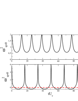
Figure 8: Behavior of the frequency $\omega^{2}_{\mathbf{q=0}}$ as a function of time for $u_{i}=0.1$ and $u_{f}=0.2$ (top panel) and $u_{f}=0.6$ (bottom panel). We see that for suitable values of $u_{f}$ the frequency can become negative for some time intervals.

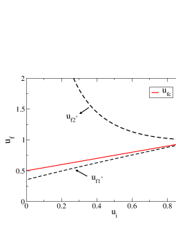
Figure 9: Behavior of the instability lines $u_{f1,2}^{\star}$ defined in the main text, as a function of $0<u_{i}<1$. We see that these lines bound a region of the phase diagram around the mean field critical line $u_{fc}$ where fluctuations grows exponentially in time. This region shrinks upon approaching $u_{i}\rightarrow 1$ while becoming wider and wider in the opposite regime of quenches from a non interacting Fermi system.

In particular, by looking at the mean field dynamics, it is easy to realize that there is a whole region of quenches, just around the dynamical transition, for which an instability in the fluctuation spectrum may occur. This region of unstable modes is bounded by two lines $u_{f1}^{\star}$, $u_{f2}^{\star}$ whose behavior is plotted in figure 9. The line $u_{f2}^{\star}$ can be obtained analytically by simple means and reads

$$u_{f2}^{\star}=\frac{\displaystyle 1+u_{i}^{2}}{\displaystyle 2u_{i}}\,.$$ (110)

As a result of this analyis we conclude that for quenches below and above these instability lines we can use the spin wave approximation to compute corrections to quantum dynamics, since all $\mathbf{q}$-modes are stable. As opposite for quenches around the critical mean field line part of the spectrum becomes unstable. Conversely, we previously found that the same method is, at least, well defined when quenching from the Mott insulator down to the Mott transition. We believe that this difference is not accidental and that the dynamics of quantum fluctuations quenching from the metallic side is poorly described by the Hamiltonian (106). The metallic phase corresponds in our language to the ordered phase of the Ising model, where a finite order parameter is spontaneously generated. The equations of motion (104) and (105) describe the dynamics of the condensate alone. The approach in section IV.3 implicitly assumes quantum fluctuations that follow adiabatically the evolution of the condensate. However, the quantum fluctuations must in turn affect the evolution of the condensate, a feedback that is absent in the above scheme and explains why the latter fails if the quench is big enough. Anyway, the fact that the Hamiltonian (106) become unstable before the dynamical critical point is encountered suggests that the effect of quantum fluctuations grows and it is not unlikely to modify substantially the dynamics.

V Conclusions

We have introduced a variational approach to strongly correlated electrons out of equilibrium. The idea is to give an ansatz on the time dependent many-body wave function and to obtain dynamical equations for the parameters by imposing a saddle point on the real-time action. While this strategy is widely used for non interacting fermionic systems, in the spirit of time dependent Hartree-Fock, its extension to strongly correlated electrons represents a novelty with many possibilities for further developments. Applications of this method can range from dynamics in closed quantum systems to non equilibrium transport in correlated quantum dots, for which a related variational approach for the steady has been recently proposed Lanatà (2010).

In this paper we have applied this variational scheme to the single band Hubbard model using a proper generalization of the Gutzwiller wavefunction. It is worth mentioning, however, that the method is general and can be applied also to other correlated wavefunctions, as long as a suitable numerical or analytical approach is available to calculate the variational energy controlling the classical dynamics of the variational parameters. As a first application we have studied the dynamics of the Hubbard model after a quantum quench of the interaction. This is an interesting open problem for which results have been obtained only very recently using sophisticated non equilibrium many body techniques. Remarkably, although extremely simple, our approach seems to capture many non trivial effects of the problem and shows a good overall agreement with the picture provided by DMFT. From this perspective it can be seen as a simple and intuitive mean field theory for quench dynamics in interacting Fermi systems.

Acknowledgment

We would like to acknowledge interesting discussions with G. Biroli, M. Capone, C. Castellani, E. Demler, A. Georges, D. Huse, S. Kehrein, C. Kollath, A. Mitra, D. Pekker and E. Tosatti. This work has been supported by Italian Ministry of University and Research, through a PRIN-COFIN award.

Appendix A Details on the Gutzwiller calculations at finite doping

In this appendix we describe in some detail the analyis of the mean field dynamics at finite doping. We start from the equation (33) where the phase $\phi$ is expressed in terms of $D$ using energy conservation

$$cos^{2}\phi=\frac{E_{0}-UD-2\bar{\varepsilon}\left(n-2D\right)\left(\sqrt{D+\delta}-\sqrt{D}\right)^{2}}{8\bar{\varepsilon}\left(n-2D\right)\sqrt{D\left(D+\delta\right)}}\,.$$ (111)

This result can be inserted into the equation for $D(t)$, which reads after simple differentiation

$$\frac{dD}{dt}=-8\bar{\varepsilon}\left(n-2D\right)\sqrt{D\left(D+\delta\right)}\,sin\phi\,cos\phi\,.$$ (112)

After some simple algebra we end up with a differential equation for the time-dependent double occupation whose general structure is

$$\frac{dD}{dt}=\pm\sqrt{\Gamma(D)}\,,$$ (113)

where $\Gamma(D)$ can be thought as an effective potential controlling the dynamics of $D(t)$. Its explicit expression reads $\Gamma\left(D\right)=\Gamma_{+}\left(D\right)\Gamma_{-}\left(D\right)$ where

$$\Gamma_{\pm}\left(D\right)=\pm\left[E_{0}-UD-2\bar{\varepsilon}\left(n-2D\right)\left(\sqrt{D+\delta}\pm\sqrt{D}\right)^{2}\right]\,.$$ (114)

After some lengthy but straightforward calculations it is possible to bring the function $\Gamma\left(D\right)$ to a polinomial form, namely to

$$\Gamma\left(D\right)=\gamma_{3}\,D^{3}+\gamma_{2}\,D^{2}+\gamma_{1}\,D+\gamma_{0}\,,$$ (115)

where $\gamma_{a}$’s are coefficients depending on the initial $U_{i}$ and final $U_{f}$ interactions as well as on the doping $\delta$. We first notice that for $\delta=0$ the expression for $\Gamma$ simplifies to read

$$\Gamma_{\delta=0}\left(D\right)=\left(u_{f}D-E_{0}\right)\left(E_{0}-u_{f}D+2D\left(1/2-D\right)\right)\,,$$ (116)

where the initial energy $E_{0}$ reads as in Eq. (32). It is easy to very that the effective potential has three roots $D_{i}$, $D_{\pm}$, the former corresponding to the equilibrium Gutzwiller solution at $T=0$, $D_{i}=\left(1-u_{i}\right)/4$ while the latters given respectively by

$$D_{+}=\left\{\begin{array}[]{ll}u_{f}<u_{fc}&\frac{u_{fc}-u_{f}}{2}\,,\\ u_{f}>u_{fc}&D_{i}\left(1-\frac{u_{fc}}{u_{f}}\right).\\ \end{array}\right.$$

and

$$D_{-}=\left\{\begin{array}[]{ll}u_{f}<u_{fc}&D_{i}\left(1-\frac{u_{fc}}{u_{f}}\right)\,,\\ u_{f}>u_{fc}&\frac{u_{fc}-u_{f}}{2}\,.\\ \end{array}\right.$$

In the doped case we cannot obtain expressions as simple. However we notice that $\Gamma_{+}\left(D_{i}\right)=0$, since by construction

$$E_{0}=u_{f}\,D_{i}+2\bar{\varepsilon}\left(n-2D_{i}\right)\left(\sqrt{D_{i}+\delta}+\sqrt{D_{i}}\right)^{2}\,.$$ (117)

As a consequence we can write the effective potential as

$$\Gamma\left(D\right)\equiv\left(D-D_{i}\right)\Phi\left(D\right)\,,$$ (118)

with $\Phi(D)$ that can be formally written as

$$\Phi\left(D\right)=\gamma_{3}\,D^{2}+\left(\gamma_{2}+D_{0}\gamma_{3}\right)D+\left(\gamma_{1}+D_{0}\gamma_{2}+D_{0}^{2}\gamma_{3}\right)$$ (119)

once the definition of the effective potential as a polynomial in $D$, Eq (115), is considered. From this result we obtain for the other two inversion points $D_{\pm}$ the following result

$$D_{\mp}=\frac{\left(\gamma_{2}+D_{i}\gamma_{3}\right)\mp\sqrt{\Delta}}{4u_{f}}\,,$$ (120)

with $\Delta=\left(\gamma_{2}+D_{i}\gamma_{3}\right)^{2}-4\gamma_{3}\left(\gamma_{1}+D_{i}\gamma_{2}+D_{i}^{2}\gamma_{3}\right)$. The explicit expression for the coefficients $\gamma_{a}$ can be easily found after some simple but lengthy algebra. These read

$$\left\{\begin{array}[]{lll}\gamma_{3}&=&-2u_{f}\\ \gamma_{2}&=&-u_{f}^{2}+2E_{0}+u_{f}\left(1-2\delta\right)-\delta^{2}/4\\ \gamma_{1}&=&2u_{f}E_{0}+\frac{n\delta^{2}}{4}+\frac{u_{f}n\delta}{2}-E_{0}\left(1-2\delta\right)\end{array}\right.$$

with $E_{0}$ given by Eq. (117). It is interesting to note that all the dependence from the initial interaction $u_{i}$ is hidden into the Gutzwiller equilibrium solution $D_{i}$. The qualitative analysis can proceed along the same lines as in the previous section, the only difference being that $D_{i}$ is not known analytically. By solving the equilibrium Gutzwiller problem at finite doping (see appendix) we can easily obtain $D_{i}$, hence $D_{\mp}$ through Eq (120). When inserted back into the previous results for $\mathcal{T}$ and $\mathcal{A}$ we find further evidence that no singularity emerges for any finite $\delta$ in those quantities, which nevertheless features some signature of the zero doping criticality. In particular both $\mathcal{T}$ and $\mathcal{A}$ are smooth functions displayng a sharp peak around $u_{fc}$.

References

- Bloch et al. (2008) I. Bloch, J. Dalibard, and W. Zwerger, Rev. Mod. Phys. 80, 885 (2008).
- Jordens et al. (2008) R. Jordens, N. Strohmaier, K. Gunter, H. Moritz, and T. Esslinger, Nature 451 (2008).
- Schneider et al. (2008) U. Schneider, L. Hackermuller, S. Will, T. Best, I. Bloch, T. A. Costi, R. W. Helmes, D. Rasch, and A. Rosch, Science 322, 1520 (2008).
- Strohmaier et al. (2010) N. Strohmaier et al., Phys. Rev. Lett. 104, 080401 (2010).
- Rosch et al. (2008) A. Rosch, D. Rasch, B. Binz, and M. Vojta, Phys. Rev. Lett. 101, 265301 (2008).
- Rapp et al. (2010) A. Rapp, S. Mandt, and A. Rosch, Phys. Rev. Lett. 105, 220405 (2010).
- Calabrese and Cardy (2006) P. Calabrese and J. Cardy, Phys. Rev. Lett. 96, 136801 (2006).
- Barmettler et al. (2009) P. Barmettler, M. Punk, V. Gritsev, E. Demler, and E. Altman, Phys. Rev. Lett. 102, 130603 (2009).
- Kollath et al. (2007) C. Kollath, A. M. Läuchli, and E. Altman, Phys. Rev. Lett. 98, 180601 (2007).
- Rigol et al. (2008) M. Rigol, V. Dunjko, and M. Olshanii, Nature 452 (2008).
- Biroli et al. (2010) G. Biroli, C. Kollath, and A. M. Läuchli, Phys. Rev. Lett. 105, 250401 (2010).
- Gogolin et al. (2011) C. Gogolin, M. P. Müller, and J. Eisert, Phys. Rev. Lett. 106, 040401 (2011).
- Eckstein, M. et al. (2009) Eckstein, M., Hackl, A., Kehrein, S., Kollar, M., Moeckel, M., Werner, P., and Wolf, F.A., Eur. Phys. J. Special Topics 180, 217 (2009).
- Barmettler et al. (2010) P. Barmettler, M. Punk, V. Gritsev, E. Demler, and E. Altman, New Journal of Physics 12, 055017 (2010).
- Cazalilla and Rigol (2010) M. A. Cazalilla and M. Rigol, New Journal of Physics 12, 055006 (2010).
- Polkovnikov et al. (2010) A. Polkovnikov, K. Sengupta, A. Silva, and M. Vengalattore, arXiv:1007.5331 (2010).
- Hubbard (1963) J. Hubbard, Proceedings of the Royal Society of London. Series A. Mathematical and Physical Sciences 276, 238 (1963).
- Gutzwiller (1963) M. C. Gutzwiller, Phys. Rev. Lett. 10, 159 (1963).
- Kanamori (1963) J. Kanamori, Progress of Theoretical Physics 30, 275 (1963).
- Moeckel and Kehrein (2008) M. Moeckel and S. Kehrein, Phys. Rev. Lett. 100, 175702 (2008).
- Moeckel and Kehrein (2009) M. Moeckel and S. Kehrein, Annals of Physics 324, 2146 (2009), ISSN 0003-4916.
- Eckstein et al. (2009) M. Eckstein, M. Kollar, and P. Werner, Phys. Rev. Lett. 103, 056403 (2009).
- Eckstein et al. (2010) M. Eckstein, M. Kollar, and P. Werner, Phys. Rev. B 81, 115131 (2010).
- Schiró and Fabrizio (2010) M. Schiró and M. Fabrizio, Phys. Rev. Lett 105, 076401 (2010).
- Huber and Rüegg (2009) S. D. Huber and A. Rüegg, Phys. Rev. Lett. 102, 065301 (2009).
- Rüegg et al. (2010) A. Rüegg, S. D. Huber, and M. Sigrist, Phys. Rev. B 81, 155118 (2010).
- Sciolla and Biroli (2010) B. Sciolla and G. Biroli, Phys. Rev. Lett 105, 220401 (2010).
- Gambassi and Calabrese (2010) A. Gambassi and P. Calabrese, arXiv:1012.5294 (2010).
- Bünemann et al. (1998) J. Bünemann, W. Weber, and F. Gebhard, Phys. Rev. B 57, 6896 (1998).
- Fabrizio (2007) M. Fabrizio, Phys. Rev. B 76, 165110 (2007).
- Negele and Orland (1998) J. W. Negele and H. Orland, Quantum Many-Particle Systems (Advanced Book Classics, 1998).
- Seibold and Lorenzana (2001) G. Seibold and J. Lorenzana, Phys. Rev. Lett. 86, 2605 (2001).
- Moeckel (2009) M. Moeckel, PhD Thesis (2009).
- de’Medici et al. (2005) L. de’Medici, A. Georges, and S. Biermann, Phys. Rev. B 72, 205124 (2005).
- Hassan and de’ Medici (2010) S. R. Hassan and L. de’ Medici, Phys. Rev. B 81, 035106 (2010).
- Georges et al. (1996) A. Georges, G. Kotliar, W. Krauth, and M. J. Rozenberg, Rev. Mod. Phys. 68, 13 (1996).
- Lanatà (2010) N. Lanatà, Phys. Rev. B 82, 195326 (2010).