Absorbing State Phase Transition in presence of Conserved Continuous Local Field

Abstract

We study absorbing state phase transition in one dimension in presence of a conserved continuous local field (CCLF) called energy. A pair of sites on a lattice is said to be active if one or both sites posses more energy than a pre-defined threshold. The active pair of sites are allowed to redistribute their energy following a stochastic rule. We show that, the CCLF model undergoes a continuous absorbing state transition when energy per site is decreased below a critical value. The critical exponents are found to be different from those of DP.

A state is called absorbing if it is impossible to leave the state. Existence of one or more absorbing configurations in a system raises a possibility of non-equilibrium phase transition between an active and an absorbing state AAPTBook . Such absorbing state phase transitions (APT) are encountered in a variety of fields, which includes percolation, spreading and chemical kinetics DPBook . Numerous physical phenomena, like forest fire ff , epidemics epi , transport in random media rm , synchronization sync and chromatography can be modeled as APT. The corresponding critical behaviour forms a universality class of APT, formally known as the directed percolation (DP)-class, which has been realized DPexp convincingly in ($2+1$) dimension.

Long ago, it has been conjectured by Grassberger and Janssen DPconj that in absence of any special symmetry or conservation law, a continuous phase transition into a single absorbing state governed by a fluctuating scalar order parameter, belongs to the DP universality class. Special symmetries, like particle-hole symmetry u9 , conservation of parity u10 , and symmetry between different absorbing states u11 lead to different universalities. Also, conserved lattice gas models u14 and conserved threshold transfer process (CTTP)cttp , where the activity field is coupled to the conserved density, show critical behaviour different from DP. The DP-conjecture has raised the question, ‘can systems with multiple absorbing states be in DP universality class?’ In the pair contact process (PCP), initially introduced by Jensen pcp , the number of absorbing configurations grow to infinity with the system size. However, numerical simulations show that the critical behaviour is same as that of DP, which is further supported by phenomenological theories pcpMunoz . Other models, like the threshold transfer process m13, and dimer reaction ̵͓ models m14, which have infinitely many absorbing states(IMAS), also show static critical exponent same as DP, whereas the dynamical exponents (that characterize the spreading of localized perturbations) are non-universal staticDP; they depend on the nature of the absorbing states and initial conditionsOdor. Additional conservation laws, like parity mendes, can change the static exponents.

More recent studies of Dickman and coworkers fes-soc have renewed the interest in APT in systems having IMAS. They were able to show that the scaling behavior observed in sandpile models of self-organized criticality soc, is entirely governed by an underlying absorbing state transition into IMAS existing in equivalent fixed energy sand pile models (FES)doubt. Corresponding universal behaviour, which are different from DP, are attributed to the presence of coupling of the order parameter to the conserving height field fes. However certain specific perturbations, like “stickiness” dd-pk, can drive these models to have critical behaviour same as DP.

In all these models discussed above, the number of absorbing states in a finite system is countable and grow exponentially to infinity in the thermodynamic limit. Models with continuous local field variable may show critical behaviour different from DP as (i) there is a possibility of having uncountably infinite number of absorbing states in these systems (even when the system size is finite) and (ii) as argued by Grassberger a9, while for continuous variables one has “incomplete death” discrete systems do not allow such a process. However, the biological evolution model (BEM) lipowsky, which has a continuous dynamical variable, show DP-critical behaviour. Whereas the coupled map lattice models, where phase transition occurs to a synchronized (absorbing) phase, follow either DP or Karder-Parisi-Zhang universality class kpz, or a first order transition pkFOT depending on the non-linearity of the map pk6. Exactly which microscopic ingredients can make an absorbing state transition not belong to the DP class is an open and challenging problem.

In this article we study a model in one dimensional lattice where the dynamical variables at the lattice sites, called energy, are continuous and their sum is conserved. They are updated pairwise, when one of the variable crosses a threshold value. We show that the system undergoes an absorbing state phase transition when the total energy crosses a critical value. Study of several variations of the models show that the critical behaviour of these systems is robust and forms a new universality class different from DP.

The model is defined on a one dimensional lattice with periodic boundary condition with sites labeled by $i=1,2\dots L.$ The dynamical variable called energy $E_{i}$, at each site $i$, is continuous and satisfies $E_{i}=E_{i+L}$ (periodic boundary condition). A pair of neighbouring sites are called active when energy of one or both the sites cross a threshold value $w$. Otherwise, $i.e.$ when both sites have energy less than $w$, they are inactive. Only the active pairs are allowed to exchange energy through an energy conserving dynamics,

$$E_{i} \to \lambda E_{i}+\epsilon(1-\lambda)(E_{i}+E_{j})$$ (1)

$$E_{j} \to \lambda E_{j}+(1-\epsilon)(1-\lambda)(E_{i}+E_{j}),$$ (2)

where $\lambda$ is a parameter of the model and $\epsilon$ is a random number distributed uniformly in $(0,1)$. Clearly the total energy $E=\sum_{i}E_{i}$ is conserved by this dynamics.

A special case of the model, $w=0$ corresponds to the kinetic model of markets introduced by Chakraborti and Chakrabarti (CC) cc in the literature of econophysics, where $E_{i}$ is considered as wealth of an agent $i$ who can interact with any other agent $j$ (not necessarily its neighbour). Naturally, in this mean-field model the parameter $\lambda$ denotes the savings propensity. Variations of these models with variable savings propensity CCM, provide the first explanation pkCCM ‘why tails of the wealth distribution follow a power law called Pareto law Pareto’. Again, when $\lambda=0$, the distribution of energy (or wealth) follows a Gibb’s distribution yv which has been observed in distribution of income-tax return of individuals in several countries tax.

In fact $\lambda=0$ case has been studied earlier Kipnis on a lattice, in context of heat conduction, as a model of collisional dynamics of particles. First we consider this case $\lambda=0$ with a finite threshold $w$ (taken as $w=1$, without loss of generality). Note, that a different threshold $w\neq 1$ would shift the transition point linearly.

To study the properties of this model, particularly possibility of phase transition and critical behaviour, we used Monte Carlo simulations. First let us define local activity field $s_{i}=0$ when the neighbouring sites $i$ and $i+1$ are inactive, $i.e.$ when both the sites have less than unit amount of energy. Or otherwise $s_{i}=1$ (the bond joining $i$ and $i+1$ is active). Clearly, the activity (or the energy exchange) does not die out when energy density $e=\frac{1}{L}\sum_{i}E_{i}$ is larger than $1$, as in this case the system has at least one active bond; starting from any arbitrary configuration, the density of active bonds $\rho(t)=\langle s_{i}\rangle$, reaches a stationary value $\rho_{s}$ as $t\to\infty$. Whereas for small energy density $e\ll 1$, the activity is expected to die out, because it is highly improbable to have macroscopic number of sites with energy larger than $w$. This indicates that there may be an absorbing state phase transition at $e_{c}<1$.

Figure 1: (Color online) The order parameter $\rho_{s}$ as a function of $e$. In log scale, $\rho_{s}$ is found to be linear in $(e-e_{c})$ by choosing $e_{c}=0.750(8).$ Any small change (in steps of $\delta=0.0005$) gives deviation from linearity (see inset (b)). Inset (a) shows that the orderparameter vanishes as $\rho_{s}\sim(e-e_{c})^{\beta}$, with $\beta=0.465$, which is visibly different from $\beta_{CTTP}=0.382.$ Here, the system size is $L=10^{4}.$

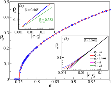
In Fig. 1, we have plotted the steady state density of active sites $\rho_{s}$ as a function of energy density $e.$ It is evident that $\rho_{s}$ takes a nonzero value as $e$ crosses $e_{c}$. $\rho_{s}$ is plotted in log scale as a function of $(e-e_{c})$ show a straight line by choosing the critical value $e_{c}=0.750(8)$ (see Fig. 1(b)). The orderparameter exponent $\beta=0.46(5)$, defined from the relation $\rho_{s}\sim(e-e_{c})^{\beta}$, is clearly different (Fig.1(a)) from that of $\beta_{CTTP}=0.382$.

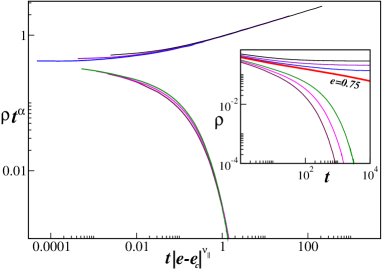
One can obtain a few other exponents from the decay of $\rho(t)$ from a fully active configuration with $\rho(0)=1.$ After an initial decay $\rho(t)\sim t^{-\alpha}$ it approaches the steady state value $\rho_{s}$ in the $t\to\infty$ limit. So $\rho$ must scale as

$$\rho(t,e)=t^{-\alpha}{\cal F}\left(t^{1/\nu_{\parallel}}(e-e_{c})\right).$$ (3)

Thus, one expects that $\rho(t)$ for different values of $e$ (shown in the Fig. 2) collapse into a single scaling function ${\cal F}$, when $t^{\alpha}\rho(t)$ is plotted against $t|e-e_{c}|^{\nu_{\parallel}}$ in log scale. The main figure here shows the data collapse when we use $\alpha=0.19(5)$, $\nu_{\parallel}=2.64.$ Since at the critical point $\rho(t,e_{c})=t^{-\alpha}{\cal F}(0)$, one can obtain both $e_{c}$ and $\alpha$ directly. Resulting $e_{c}$ and $\alpha$ are consistent with those obtained from the data collapse. Again, in $t\to\infty$ limit, $\rho$ vanishes as $|e-e_{c}|^{\beta}$. This can happen only when ${\cal F}(x)\sim x^{\beta/\nu_{\parallel}}$; thus

$$\alpha=\beta/\nu_{\parallel}.$$

Since all three exponents $\beta$, $\alpha$ and $\nu_{\parallel}$ are calculated independently, one can check if the above scaling relation holds. In fact, it holds to a great accuracy for the values of $\beta$, $\alpha$ and $\nu_{\parallel}$ calculated here.

Figure 2: (Color online) Inset : Decay of $\rho(t)$ from a fully active state to the steady state value $\rho_{s}$ is shown in the inset for $L=1000$ and $e=0.65,0.67,0.69,0.75,0.77,0.8,$ and $0.85$ . Main figure : Data collapse for off-critical simulations according to the scaling form Eq. (3) is obtained for $\alpha=0.19(5)$ and $\nu_{\parallel}=2.64.$

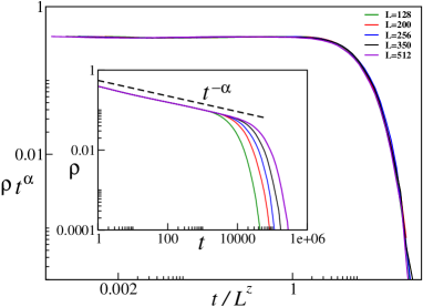
Now we turn our attention to the finite size scaling of $\rho(t)$ at the critical point. Again, from a fully active state $\rho(t,L)$ decays as $t^{-\alpha}$, indicating a scaling form

$$\rho(t,L)=t^{-\alpha}{\cal G}(t/L^{z}),$$ (4)

where $z$ is the dynamic exponent. Thus, one expects that $\rho(t)$ for different values of $L$ collapse to a single function when plotted against $t/L^{z}$. This is described in Fig. 3. The inset there shows variation of $\rho(t)$ for different $L=128,200,256,350,512$, which were made to collapse to a single function using $\alpha=0.19(5)$ and $z=1.38(1)$. Now, assuming the scaling relation $z=\nu_{\parallel}/\nu_{\perp},$ one can obtain $\nu_{\perp}=\beta/\alpha z.$

The exponents we obtained using Monte-Carlo simulations are listed in Table 1, along with the exponents of DP, BEM and CTTP. Clearly, the exponents of CCLF model are quite different from the DP. Even the static exponents, which are believed staticDP to be same as that of DP for models with multiple absorbing sates, are now different. Though some of the exponents are close to the same obtained for CTTP, particularly the order parameter exponent $\beta$, and the spreading exponent $\alpha$ are very different. Since the value of $\beta$ crucially relies on the estimation of the critical point, we provide a careful study of $e_{c}$ based on Ref. note1 in Appendix-I. From this analysis it is concluded, beyond reasonable doubts, that $\beta=0.46(5)$ and thus the phase transition in CCLF model belong to a new universality class.

One can possibly reason it to the existence of a continuous conserved field. Further study in this direction is required to identify, what made this absorbing state phase transition different from the usual ones.

Figure 3: (Color online) The decay of $\rho(t)$ at $e_{c}=0.750$ from a fully active state, averaged over $10^{4}$ ensembles, is shown in the inset for different $L=128,200,256,350,$ and $512$. A line with slope $\alpha=0.195$ is drawn to emphasize that $\rho(t)\sim t^{-\alpha}.$ The main figure shows the data collapse for finite size scaling Eq. (4) using $z=1.381.$

Table 1: Critical exponents of DP, BEM and CCLF model.

	$\beta$	$\nu_{\parallel}$	$\alpha$	$z$
DP DPBook	0.276	1.733	0.159	1.581
BEM lipowsky	0.276	1.067	.259	1.364
CCLF	0.46(5)	2.6(4)	0.19(5)	1.38(1)
CTTP cttp	0.382	2.45	0.141	1.393

In the following we discuss some possible directions of studies which may explain the new universality. The model studied here, is quite similar to the sandpile models soc of self organized criticality, except that the local field variables in CCLF model are continuous. It has been pointed out in Ref. dd-pk, that although the critical behaviour of sandpile models crucially depends on the details of the dynamics and the spatial dimension, they are unstable to certain specific perturbation (called stickiness) and flow generically to the DP universality class. It would be interesting to ask, if the model studied here is unstable to perturbations. Some generic variations, which may change the critical behaviour of CCLF, are discussed below.

The bulk dynamics of CC model ($\lambda\neq 0$) does not satisfy detailed balance, as for any arbitrary $(E_{i},E_{j})\to(E_{i}^{\prime},E_{j}^{\prime})$ it is not possible to have $(E_{i}^{\prime},E_{j}^{\prime})\to(E_{i},E_{j}).$ Thus, $\lambda\neq 0$ is a singular perturbation and it may change the universality class. The quenched disorder, introduced by taking a distributed savings propensity $\{\lambda_{i}\}$ CCM may also change the critical behaviour.

In conclusion, we have studied absorbing state phase transition in a model with conserved continuous local field (CCLF). In one dimension, the model is defined on a lattice with sites $i$ having continuous variable $E_{i}$ called energy. Two neighbouring sites $i$ and $i+1$ can exchange energy when one or both sites have energy larger than a predefined threshold $w.$ The exchange dynamics is similar to the wealth exchange model cc studied earlier, by considering $E_{i}$ as wealth of the agent $i$. Clearly, the system is active (i. e. surely some of the neighbouring sites keep exchanging their wealth) when the energy density $e$ is larger than $w$ (set to be unity, without loss of generality). Whereas for $e\ll 1$ it is improbable to get macroscopic number of sites which have wealth larger than $w$ indicating that the system falls into one of the uncountably infinite number of absorbing states. We show that, CCLF model undergoes a continuous phase transition at $e_{c}=0.750(8)$ with critical exponents $\beta=0.46(5)$, $\nu_{\parallel}=2.6(4)$, $\alpha=0.19(5)$, and $z=1.38(1)$, which are very different from those of DP. However earlier studies staticDP, both numerical and analytical, have shown that the static exponents of absorbing state transition to infinitely many absorbing states are same as those of DP, whereas dynamic exponents differ. It is surprising, that in CCLF model, even the static exponents differ from DP and form a new universality class. One may argue that the existence of the conserved field is responsible for this behaviour. But, this can not be the sole argument as recent studies dd-pk show that it is possible to get DP behaviour in presence of conserved field(s).

Appendix-I

The numerical estimation of the critical exponents of CCLF model are listed in Table-I. The critical exponents $\nu_{\parallel}$ and $z$ are quite close to that of CTTP, whereas $\beta$ and $\alpha$ are substantially different. The main claim of this article, that CCLF model form a new universality class, is based on this difference. Since the value of $\beta$ strongly depends on the the critical point , here we estimate $e_{c}$ through a careful and systematic numerical analysis based on Ref. note1.

Figure 4: (Color online) (a) $\rho$ versus $t$ for $e=0.76$ and $0.765$ are fitted with the scaling form (6). (b) $A^{-1}\rho t^{\alpha}-1$ as a function $t$ in log scale is linear for both $e=0.76$ and $0.765$ when $A=2.64$; the solid lines indicates a power-law $t^{1/\nu_{\parallel}}$ with $\nu_{\parallel}=2.64$ and coefficients $0.0178$ and $0.0269$ respectively. From these coefficients we find that $B=1.82$ and $e_{c}=0.75022.$ The inset of (a) shows that $\rho(t,e_{c})$ obtained from $\rho(t,e=0.76)$ using Eq. (7) varies as $t^{-\alpha}$ with $\alpha=0.19$, when $e_{c}$ is taken as $0.7503.$ Here $L=1024$.

Near the critical point, the order parameter $\rho(t,e)$ follow Eq. (3); thus

$$\rho(t,e) = At^{-\alpha}(1+B(e-e_{c})~{}t^{1/\nu_{\parallel}})$$ (5)

$$\simeq \rho(t,e_{c})(1+B(e-e_{c})~{}t^{1/\nu_{\parallel}})$$ (6)

where we have used the Taylor’s expansion of scaling function ${\cal F}(x)$ at $x=0$ upto the first term, $i.e.~{}{\cal F}(x)=A(1+Bx).$ Clearly, this functional form is valid for $t\ll|e-e_{c}|^{-\nu_{\parallel}}.$

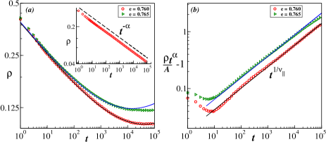
Using this functional form, which is valid for $t\ll|e-e_{c}|^{-\nu_{\parallel}},$ one can obtain $\nu_{\parallel}$ by suitably choosing $A$ such that $A^{-1}\rho(t,e)t^{\alpha}-1$, as a function of $t$, is linear in log scale; the slope and the $y$-intercept determine the $\nu_{\parallel}$ and $B(e-e_{c})$ respectively. For a system of size $L=1024$, $\rho$ is shown in Fig. 4 (a) for two different values of $e=0.76$ and $0.765$. Figure 4(b) shows that $A^{-1}\rho(t,e)t^{\alpha}-1$ is linear in log scale for both values of $e$, with $\alpha=0.19$ and $A^{-1}=2.64$. The slope of both the straight-lines turns out to be $1/\nu_{\parallel}=0.379$, which is consistent with $\nu_{\parallel}=2.6(4)$ obtained earlier from the data-collapse. From their $y$-intercepts we get, $B(e-e_{c})=0.0178,0.0269$ respectively for $e=0.76$ and $0.765,$ which provide $e_{c}=0.75022$ and $B=1.82.$ Using these parameters, we have calculated $\rho(t,e)$ as a function of $t$ for $e=0.76,0.765$ (shown as solid lines in Fig. 4(a)). The discrepancy for large $t$, in case of $e=0.765$ is due to the fact that we have approximated ${\cal F}(x)$ in Eq. (6) up to the linear order.

A better estimation of $e_{c}$ can be done now by using Eq. (6),

$$\rho(t,e_{c})=\frac{\rho(t,e)}{1+B(e-e_{c})~{}t^{1/\nu_{\parallel}}}.$$ (7)

Since we know the value of $B$ and $\nu_{\parallel}$, $e_{c}$ can be used as a fitting parameter in the above equation such that $\rho(t,e_{c})$ obtained from the numerical values of $\rho(t,e)$ using Eq. (7) shows a power-law. The inset of Fig. 4 (a) shows that $\rho(t,e_{c})$, obtained from $\rho(t,e=0.76)$ by choosing $e_{c}=0.7503$, decays algebraically for four decades with exponent $\alpha=0.19.$ Thus the final estimate of the critical point for $L=1024$ is $e_{c}=0.7503.$

Figure 5: (Color online) (a) $\rho_{s}$ as a function of $e$ for different $L=128,256,512,1024$ and $10^{4}$. Difference in $\rho_{s}$ is visible only after sufficient magnification. (b) $\rho_{s}$ for different $L$ are merged onto the same for $L=10^{4}$ by using Eq. (8). The inset here show variation of $e_{c}(L)$ with $1/L$, which is linear. The critical value obtained for $L=1024$ following Ref. note1 is shown as a circle. The asymptotic value of the critical point, extrapolated for $L\to\infty$ is $e_{c}=0.7508.$

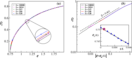
In general, the order parameter and thus the critical point depends strongly on system size $L$. In Fig. 5 (a), we have plotted $\rho_{s}$ as a function of $e$, for $L=128,256,512,1024$ and $10^{4}$. These curves do not show any significant dependence on $L$. The small difference can be adjusted by shifting the $x$-axis by a small amount $\delta_{L}$, which results in

$$\rho_{s}^{L}(e)=\rho_{s}^{\infty}(e+\delta_{L})\sim(e-e_{c}(L))^{\beta},$$ (8)

where $e_{c}(L)=e_{c}(\infty)-\delta_{L}.$ We calculate $e_{c}(L)$ as the value, where the log scale plot of $\rho_{s}$ versus $e-e_{c}(L)$ is linear. In fact, with these choice of $e_{c}(L)$, all the different curves of $\rho_{s}^{L}$ could be merged on to the curve for $L=10^{4}$ (see Fig. 5 (b)). The inset of Fig. 5 (b) shows the small variation of $e_{c}(L)$ with $1/L$, which asymptotically approach to $e_{c}=0.7508$ as $L\to\infty.$ Again, the value of $e_{c}$ obtained in this Appendix for $L=1024$, using a method described in Ref. note1, consistently fall on this curve (denoted by a circle in the inset of Fig. 5 (b)) .

These analysis suggest that the estimates of $e_{c}$ and the critical exponents $\beta$ and $\alpha$ do not change appreciably with system size. The current values of exponents obtained for system size $L=10^{4}$ are sufficient to conclude that the critical behaviour in CCLF model belongs a universality class different from CTTP.

References

- (1) J. Marro and R. Dickman, Non-equilibrium phase transitions in lattice models (Cambridge University Press, Cambridge, 1999);
- (2) H. Hinrichsen, Non-equilibrium Critical Phenomena and Phase Transitions into Absorbing States, Advances in Physics 49, 815 (2000); M. Henkel, H. Hinrichsen, and S. Lübeck, Non-Equilibrium Phase Transitions, Berlin: Springer (2008).
- (3) E. V. Albano, J. Phys. A 27, L881 (1994).
- (4) D. Mollison, J. Roy. Stat. Soc. B 39, 283 (1977).
- (5) S. Havlin and D. ben Avraham, Adv. Phys. 36, 695 (1987); J. P. Bouchad and A. Georges, Phys. Rep. 195, 127 (1990).
- (6) P. Grassberger, Phys. Rev. E59, R2520 (1999); V. Ahlers and A. Pikovsky, Phys. Rev. Lett. 88, 254101 (2002).
- (7) K. A. Takeuchi, M. Kuroda, H. Chaté, and M. Sano Phys. Rev. E 80, 051116 (2009); H. Hinrichsen, Physics 2, 96 (2009).
- (8) P. Grassberger, Z. Phys. B 47, 365 (1982); H. K. Janssen, Z. Phys. B 42, 151 (1981).
- (9) J. W. Essam, J. Phys. A 22, 4927 (1989).
- (10) I. Jensen, J. Phys. A 26, 3921 (1993).
- (11) H. Hinrichsen, Phys. Rev. E 55, 219 (1997).
- (12) M. Rossi, R. Pastor-Satorras, and A. Vespignani, Phys. Rev. Lett. 85, 1803 (2000).
- (13) S. Lubeck and P. C. Heger, Phys. Rev. E 68, 56102 (2003).
- (14) I. Jensen, Phys. Rev. Lett. 70, 1465, (1993); I. Jensen, Phys. Rev. E 47, R1 (1993); I. Jensen and R. Dickman, Phys. Rev. E 48, 1710 (1993).
- (15) M. A. Munoz, G. Grinstein, R. Dickman and R. Livi, Phys. Rev. Lett. 76, 451,(1996).