A spectral comparison of (379) Huenna and its satellite

Abstract

We present near-infrared spectral measurements of Themis family asteroid (379) Huenna (D$\sim$98 km) and its 6 km satellite using SpeX on the NASA IRTF. The companion was farther than 1.5^′′ from the primary at the time of observations and was approximately 5 magnitudes dimmer. We describe a method for separating and extracting the signal of a companion asteroid when the signal is not entirely resolved from the primary. The spectrum of (379) Huenna has a broad, shallow feature near 1 $\mu$m and a low slope, characteristic of C-type asteroids. The secondary’s spectrum is consistent with the taxonomic classification of C-complex or X-complex. The quality of the data was not sufficient to identify any subtle feature in the secondary’s spectrum.

1 Introduction

Since the discovery of the small moon Dactyl around (243) Ida by the Galileo spacecraft more than a decade ago, many more systems have been discovered by either indirect methods (lightcuves, e.g. Pravec et al. 2006) or direct detection (direct imaging or radar echoes, e.g. Merline et al. 1999; Margot et al. 2002; Ostro et al. 2006; Marchis et al. 2008). The study of the physical and orbital characteristics of these systems is of high importance, as it provides density measurements and clues on formation processes through models (e.g. Durda et al. 2004; Walsh et al. 2008). Primary formation scenarios include capture (from collision or close approach), and fission and mass-loss from either YORP spin up for small binary asteroids (D$<$20 km, Pravec and Harris 2007; Walsh et al. 2008) or from oblique impacts for large asteroids (D$>$100 km, Descamps and Marchis 2008).

Spectroscopic measurements of each component of multiple systems are fundamental to understand the relationship between small bodies and their companions. From high quality measurements, differences in slope and band depths provide information on composition, grain sizes, or effects of space weathering on each surface and help constrain formation scenarios. Obtaining photometric colors or spectra of the secondaries, however, is rarely possible due to the small (sub arcsecond, often less than a few tenths of an arcsecond) separation and relative faintness (often several magnitudes dimmer) of the satellites. Photometric colors of TNO binaries, which are typically of comparable size, have revealed their colors to be the same and are indistinguishable from the non-binary population (Benecchi et al. 2009). The first spectroscopic measurements of a resolved asteroid system, (22) Kalliope, are presented by Laver et al. (2009) using the Keck AO system and its integral field spectrograph OSIRIS. They find the spectra of the primary and secondary to be similar, suggesting a common origin. More recently Marchis et al. (2009) presented a comparative spectroscopic analysis of (90) Antiope based on data collected using the 8m-VLT and its integral field spectrograph SINFONI. This binary asteroid is composed of two large (D$\sim$85 km) components. A comparison of Antiope’s component spectra suggest that the components are identical in surface composition and most likely formed from the same material.

In November 2009, main-belt asteroid (379) Huenna reached perihelion, and the system had a separation of over 1.5^′′. The primary is a large (D$\sim$98 km, Marchis et al. 2008; Tedesco et al. 2002) C-type (Bus and Binzel 2002) and a member of the Themis family (Zappala et al. 1995). Its secondary (S/2003 (379) 1) was discovered by Margot (2003). With an estimated diameter of 6 km, the secondary is $\sim$5 magnitudes fainter at optical wavelengths than the primary, and it has a highly eccentric orbit (e $\sim$ 0.22) with a period of 87.60 $\pm$0.026 days (Marchis et al. 2008). This irregular orbit suggests mutual capture from disruption of a parent body or even an interloper (Marchis et al. 2008). It is not likely that the secondary formed by fragmentation of Huenna due to the YORP spinup effect, because the primary is too large for this process to be efficient (Rubincam 2000; Walsh et al. 2008). Here we present near-infrared spectral measurements of the primary and secondary and as well as a new spectral extraction method to separate them.

2 Observation and Data Reduction

2.1 Spectroscopy

We observed the (379) Huenna system on 2009 November 28 UT, and obtained near-infrared spectral measurements from 0.8 to 2.5 $\mu$m using SpeX, the low- to medium-resolution near-IR spectrograph and imager (Rayner et al. 2003), on the 3-meter NASA IRTF located on Mauna Kea, Hawaii. Observations were performed remotely from the Centre d’Observation à Distance en Astronomie à Meudon (CODAM, Birlan et al. 2004) in Meudon, France. Using the Binary Orbit Fit (BOF) algorithm from Descamps (2005) and the orbital parameters provided in Marchis et al. (2008), the secondary was expected to be located about 1.88^′′ W and 0.17^′′ N with respect to the primary at the time of our observations. The configuration of the slit (shown in Fig. 1) was thus chosen as following. The slit was first centered on the primary (position “P” in Fig. 1) and 8 spectra of 120 seconds were taken, alternated between two different positions (usually noted as ‘A’ and ‘B’) on a 0.8^′′$\times$15^′′ slit aligned in the north–south direction. We chose not to align the slit along the parallactic angle to facilitate the positioning of the slit on the secondary for these challenging observations. Next, the slit was shifted west $\sim$1.8^′′ (15 pixels; position “S” in Fig. 1) to maximize the flux from the bulge on the southwest portion of the guider image, the secondary, and minimize contamination from the light of the primary. We continued to guide on the primary while taking spectra of the secondary. Because of the long period ($\sim$87 day) of the secondary, its motion relative to the primary during our observations was negligible. We spent two hours taking spectra of 120 seconds of the secondary, although we combine and present only the 11 spectra toward the end of the night, when the seeing was lowest and the signal of the secondary was detectable. The solar-type standard star Landolt 102-1081 (Landolt 1983) was observed to remove the solar contribution from the reflected light, and an argon arc lamp spectrum was taken for wavelength calibration.

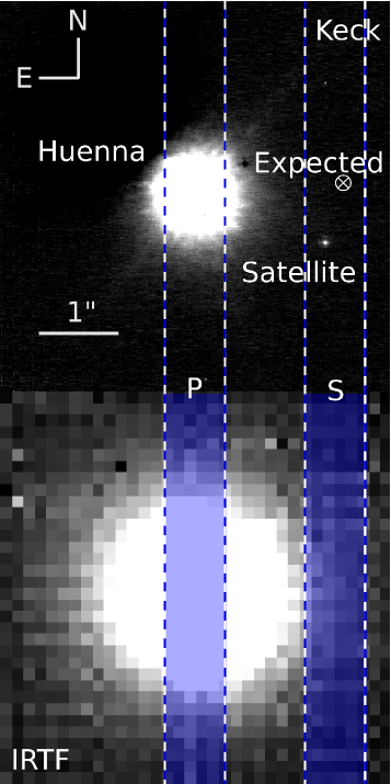
Figure 1: Observing configuration: P marks the position of the slit for observations of the primary using the IRTF observations. S marks the position for the secondary which was chosen based on the expected position of the secondary. Top: Adaptive-optics image obtained with NIRC2 at the Keck telescope. Bottom: Image obtained at the IRTF with SpeX slit-viewer, displayed at the same scale. Both images are oriented with north up and east left. The plate scale of the IRTF spectrograph and IRTF guider (slit-viewer) are 0.15 and 0.12^′′/pixel, respectively.

The dome was closed for the first two hours of the observations due to high humidity. During the beginning of the observations the seeing was around 1^′′ and humidity was high. The data we present here, however, were taken toward the end of the night when the humidity had dropped to 10% and the seeing was down to about 0.5^′′.

Reduction was performed using a combination of routines within the Image Reduction and Analysis Facility (IRAF), provided by the National Optical Astronomy Observatories (NOAO) (Tody 1993), and Interactive Data Language (IDL). A software tool called Autospex was used to streamline reduction procedures to create a bad pixel map from flat field images, apply a flat field correction to all images and perform the sky subtraction between AB image pairs. The primary spectra were combined and the final spectrum was extracted with a large aperture centered on the peak of the spectrum using the apall procedure in IRAF. The spectral extraction procedure of the satellite is described in Section 3. A wavelength calibration was performed using an argon arc lamp spectrum. The spectra were then divided by that of the standard star to determine the relative reflectance and normalized to unity at 1.215 $\mu$m.

2.2 Imaging

On the same night (see Table 1), we also observed Huenna using the Adaptive Optics system of the Keck-II telescope and its NIRC2 infrared camera (1024$\times$1024 pixels with a pixel scale of 9.94 $\times$ 10^-3 arcsec/pixel). Two Kp-band (bandwidth of 0.351 $\mu$m centered on 2.124 $\mu$m) images made of 4 coadded frames each with an integration time of 40 seconds were basic-processed using classical methods (sky subtraction, flat-field correction and bad pixel removal). In the resulting frame shown in Fig. 1 (averaged observing time 13:49:05), obtained after shift-adding these two frames, the primary is not resolved and slightly saturated. The satellite is detected with a peak SNR$\sim$23 and no motion with respect to the primary was detected over the 6 minutes of observation.

The position of the satellite as measured on the NIRC2 image (Fig. 1) is 1.67^′′$\pm$0.05^′′ W and 0.62^′′$\pm$0.05^′′ S, significantly offset from the predicted position based on the Marchis et al. (2008) orbital model (1.88^′′ W and 0.17^′′ N). This highlights the need for a refined period and adjustment for precession effects due to the irregular shape of the primary. Additional astrometric measurements are necessary to better constrain the orbital period and precession. For the spectroscopic observations on the IRTF, because the slit was oriented N-S and the displacement of the satellite in the E-W direction with respect to its expected position was only 0.2^′′ (compared to a 0.8^′′ slit), the slit was well-positioned on the satellite (see Fig. 1).

Table 1: Observations on 28 November 2009

Target	Time (UT)	Airmass	Instrument
(379) Huenna	12:56-13:08	1.31-1.37	Spex, IRTF
S/2003 (379) 1	13:13-13:56	1.40-1.75	Spex, IRTF
L102-1081	14:19-14:26	1.34-1.31	Spex, IRTF
(379) Huenna	13:46-13:52	1.6-1.75	NIRC2, Keck-II

3 Spectral Extraction of the Satellite

Given the spatial resolution of SpeX, which is limited by the atmospheric seeing, and the angular separation of (379) Huenna and its satellite at the time of our observations ($\sim$1.5^′′), the spectrum of the secondary was contaminated by diffuse light from the primary. We thus extracted both spectra (the companion and the diffuse light of the primary) at once, by adjusting a fit function at each wavelength composed of the sum of two Gaussian functions (one for each component) on top of a linear background:

$$\textrm{fit}=\frac{f_{p}}{\sqrt{2\pi\sigma^{2}}}~{}.~{}\textrm{exp}\left(\frac{-(x-c_{p})^{2}}{2\sigma^{2}}\right)+\frac{f_{s}}{\sqrt{2\pi\sigma^{2}}}~{}.~{}\textrm{exp}\left(\frac{-(x-c_{s})^{2}}{2\sigma^{2}}\right)+ax+b$$ (1)

where $x$ describes the pixels perpendicular to the wavelength dispersion direction. The 7 free parameters are: $a$ and $b$, the slope and absolute level of the background, $f_{p}$ and $f_{s}$, the maximal flux of each component centered on $c_{p}$ and $c_{s}$, respectively, and $\sigma$ the Gaussian standard deviation. In Fig. 2 we present an example of the adjustment showing both components and their sum plotted with the data.

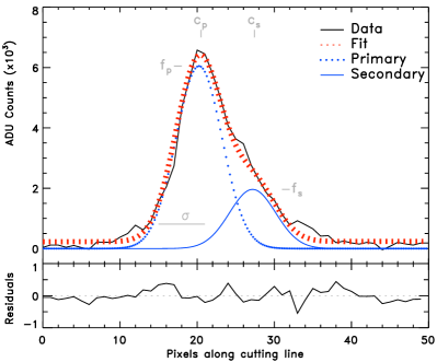
Figure 2: A cut of the (379) Huenna spectrum along a wavelength-constant line ($\lambda=1.23$ $\mu$m). Acquired data (observing time 13:58 UT) is plotted as a black solid line, and the corresponding best-fit curve is drawn as a dotted red line. Individual Gaussian functions for Huenna (primary) and its satellite (secondary) are drawn in bulleted and solid blue curves, respectively. Central positions ($c_{p}$, $c_{s}$), peak amplitudes ($f_{p}$, $f_{s}$), and Gaussian standard deviation ($\sigma$), accordingly to notation in Eq.1, are labeled for clarity. Residuals of the fit are plotted on the bottom panel.

We verified the accuracy and robustness of the extraction by examining the residuals of the fit and the evolution of the free parameters according to wavelength shown in Fig. 3. First, the angular separation between the two components, the peak of the diffuse primary light and the secondary, ($c_{p}$$-$$c_{s}$) is nearly constant, with a value of $1.04\pm 0.25$^′′, the uncertainty being mostly due to the uncertainty of the position of the secondary ($c_{s}$, see Fig. 3). This separation is the order of magnitude expected (0.62^′′ along the North-South direction, see Fig. 1).
Second, the Gaussian standard deviation ($\sigma$) follows the expected trend due to the seeing power-law dependence with wavelength. Indeed, the seeing is proportional to $\lambda^{-1/5}$, which means that the amount of diffused light from Huenna entering the slit is not the same at short (e.g. J) and long (e.g. K) wavelengths. The same effect occurs with the slit-dispersed light: in the direction perpendicular to the wavelength dispersion, the spectrum is broader at shorter wavelengths and narrower at longer wavelengths. The combined effect is a $\lambda^{-2/5}$ dependence of the standard deviation ($\sigma$). We plot in Fig. 3 the theoretical wavelength dependence function of the Gaussian standard deviation, labeled “seeing”, for a seeing value of 0.5^′′ at 0.5 $\mu$m.
We set the standard deviation of the satellite Gaussian function equal to Huenna’s to simplify the fitting algorithm. However, from the discussion above, we can expect a wavelength dependence in $\lambda^{-1/5}$ for the satellite (which is entirely covered by SpeX slit). This implies we slightly underestimate the size of the satellite Gaussian function toward longer wavelength, and thus the satellite flux, and therefore its spectral slope.
Third, the peak-to-peak amplitude measured for Huenna and its satellite corresponds to the value of $\Delta m\approx 6$ reported by Marchis et al. (2008): the ratio $f_{s}/f_{p}$ measured for the spectra is $0.4\pm 0.1$, and the amount of diffused light from Huenna entering the slit is about 1% of the overall peak amplitude of Huenna ($f_{H}$), calculated using a Gaussian profile for Huenna due to $\sim$0.5–0.6^′′ seeing, conditions similar to what we had at the end of the night. Note that $f_{H}$ is Huenna’s overall maximum, not the local peak we measure for dispersed light that we call $f_{p}$.
Finally, the background level ($b$), mimics the spectral behavior of Huenna, whose diffused light dominated the light entering the slit, as expected. The amount of diffused light entering the slit 1^′′ from $c_{p}$ (a separation corresponding to 2 $\sigma$) is about 10^-5 $\times f_{H}$, corresponding to $\approx f_{p}$/250 (under the same seeing assumptions).

We also test our extraction method by comparing the high quality spectrum of the primary while centered on the primary extracted by both methods. In the IRAF reduction, the center peak is identified, an aperture width is chosen, and all the flux within that region is summed. In our method we fit Gaussian functions to the flux. An additional error is introduced in our extraction method because the fit functions can slightly over or underestimate the flux. The largest error is introduced before 1 $\mu$m and past 2.3 $\mu$m as is shown in the top panel of Fig. 3. The spectra are generally consistent, although the slope of the spectrum from the new extraction method is lower (0.70$\pm$0.09 vs. 1.04$\pm$0.05) and we do not see the 1 micron band as clearly because of the poorer fit of the function at shorter wavelengths. This suggests that the errors in the slope from the Gaussian extraction are greater than the formal errors listed. The spectra of the diffuse primary and the secondary have a low signal-to-noise ratio and thus high errors due to the low flux and the limited time when the seeing was sufficiently low.

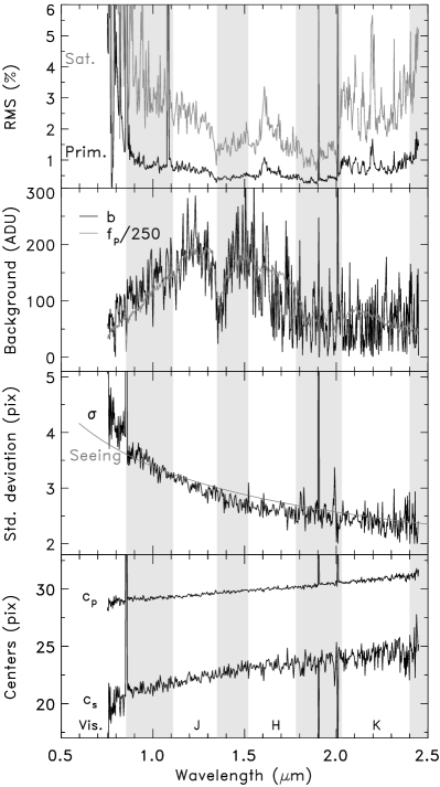
Figure 3: Parameters of the spectral extraction plotted as function of the wavelength.The gray areas represent the wavelength ranges affected by telluric absorptions, and we labeled the atmospheric windows with their usual designation (visible, J, H, and K). From bottom to top. Sub-panel 1: position of the two Gaussian centers, Huenna ($c_{p}$) and its satellite ($c_{s}$). Sub-panel 2: the Gaussian standard deviation ($\sigma$) compared to the atmospheric theoretical seeing (see text). Sub-panel 3: the background level ($b$) compared to a fraction of Huenna flux ($f_{p}$). Sub-panel 4: the residual of the fit, displayed as percent of the peak value of the spectra ($f_{p}$ and $f_{s}$ for Huenna and its satellite respectively).

4 Results

Table 2: Slope Measurements

Object1	Slope 0.9-2.4 $\mu$m	Slope 0.9-1.3 $\mu$m	Slope 1.4-2.4 $\mu$m
	[%/(103 Å)]	[%/(103 Å)]	[%/(103 Å)]
(379) IRAF	1.04$\pm$0.05	0.70$\pm$0.02	1.29$\pm$0.02
(379) Gauss	0.70$\pm$0.09	-1.20$\pm$0.05	0.86$\pm$0.05
(379) Diffuse	2.34$\pm$0.59	2.53$\pm$0.38	1.45$\pm$0.38
S/2003 (379) 1	2.51$\pm$1.17	3.41$\pm$0.77	1.20$\pm$0.77

The spectra of Huenna and its companion are presented in Figure 4. Slopes are calculated between 0.9 and 2.4 $\mu$m using a chi-square minimizing linear model (using the IDL routine linfit) and are listed in Table 2 with their formal errors for various wavelength ranges. The telluric regions from 1.3 to 1.4 $\mu$m and from 1.8 to 2.0 $\mu$m were excluded from the calculation. A spectrum of the primary published by Clark et al. (2010) is taxonomically in agreement with our spectrum, also a C-type, however the band minima positions differ (1.020 $\mu$m versus 1.045 $\mu$m for our data). The slope of our spectrum is also lower than the previously published data, although they agree within the errors, 1.04$\pm$0.55 and 1.94$\pm$0.53 %/10³ Å. An additional error of 0.5 %/10³ Å is added to these slopes because in this case we are comparing data from different nights using different standard stars.

Figure 4: Top section: From top to bottom: The spectrum of the primary with the slit centered on the primary reduced using IRAF; the same data reduced using the new Gaussian method presented here; the spectrum of the primary with the slit centered on the secondary measuring the diffused light; and the spectrum of the secondary. The spectra are plotted with one sigma errors and are normalized to unity at 1.215 $\mu$m and are shifted by -0.5,+1.5,+2.5, and +2.8, respectively. Bottom section: The ratio of the secondary and diffuse primary spectra both with the slit centered on the secondary.

The spectrum of the secondary is consistent with a C-complex or X-complex spectrum. The C- and X-complexes are broad umbrella terms for B-, C-, Cb-, Cg-, Cgh-, Ch-types and X-, Xc-, Xe-, and Xk- types, respectively. Without accompanying visible data, C-complex and X-complex spectra are indistinguishable except in the case of the presence of a broad 1 $\mu$m feature indicating C-type (DeMeo et al. 2009). As can be seen in Table 2 the slopes of the spectra of the secondary and the diffuse light of the primary are greater than the slope of the primary spectrum even considering the large error. Particularly, the slopes are much greater in the shorter wavelength region, while the slopes are all relatively consistent in the higher wavelength region. Because this slope effect is seen for both spectra, we suspect it is not due to any compositional differences but rather to the observational circumstances.

Differences in slope could be caused by atmospheric differential refraction which varies as a function of wavelength and is stronger at shorter wavelengths (Filippenko 1982). For our observations, the slit was oriented in the north-south direction rather than along the parallactic angle. We chose this orientation to facilitate the positioning of the slit on the secondary while reducing the contamination of diffuse light from the primary. However, this slit orientation could introduce slope effects. Airmass differences at the times of the observations are likely the biggest contributor to slope effects. The airmass was 1.3 when centered on the primary and 1.4-1.7 when centered on the secondary. Because the airmass of the standard star was 1.34 at the time of observation, effects of atmospheric refraction were not entirely removed for the observations when centered on the secondary.

Considering the effects of airmass and parallactic angle that introduce an additional slope affect to the data, we are unable to be certain whether the slope of the secondary is consistent with the primary. This allows several possible formation scenarios. The satellite could be a fragment from a former parent body that was disrupted to form Huenna and the secondary. The satellite could be a member of the Themis family that was captured into an eccentric orbit around Huenna. Although more unlikely, it could also be a captured interloper of similar taxonomic type. We are confident, however, that the satellite is not of a significantly different taxonomic type.

We have presented the third resolved spectrum of a moonlet satellite of a multiple asteroid system, the first being (22) Kalliope from Laver et al. (2009) and the second, (90) Antiope (Marchis et al. 2009). Our innovative extraction method allows us to derive the spectra of the satellite (with a magnitude difference of 5 and distance of 1.5^′′) and the primary, and this method could be used for similar future projects. These results show the capability of a medium-size telescope to aid in the measurement of multiple system asteroids with large separations. Further observations with larger telescopes, particularly those equipped with adaptive optics, can be used to perform the similar measurements for multiple asteroid systems which are not easily separable (angular distance $<$1^′′), and will be useful to constrain formation scenarios.

5 Acknowledgments

We are grateful to Andy Boden, Gaspard Duchene, Shri Kulkarni, Bruce Macintosh, and Christian Marois for helpful discussions and for sharing results from their data. This research has made use of NASA’s Astrophysics Data System. FD y BC consideran que este proyecto fue una huenna oportunidad para trabajar juntos. The authors wish to recognize and acknowledge the very significant cultural role and reverence that the summit of Mauna Kea has always had within the indigenous Hawaiian community. We are most fortunate to have the opportunity to conduct observations from this mountain.

References

- Benecchi et al. (2009) Benecchi, S. D., Noll, K. S., Grundy, W. M., Buie, M. W., Stephens, D. C., Levison, H. F., Mar. 2009. The correlated colors of transneptunian binaries. Icarus 200, 292–303.
- Birlan et al. (2004) Birlan, M., Barucci, M. A., Vernazza, P., Fulchignoni, M., Binzel, R. P., Bus, S. J., Belskaya, I., Fornasier, S., 2004. Near-IR spectroscopy of asteroids 21 Lutetia, 89 Julia, 140 Siwa, 2181 Fogelin and 5480 (1989YK8), potential targets for the Rosetta mission; remote observations campaign on IRTF. New Astronomy 9, 343–351.
- Bus and Binzel (2002) Bus, S. J., Binzel, R. P., Jul. 2002. Phase II of the Small Main-Belt Asteroid Spectroscopic Survey, A Feature-Based Taxonomy. Icarus 158, 146–177.
- Clark et al. (2010) Clark, B. E., Ziffer, J., Nesvorny, D., Campins, H., S., R. A., Hiroi, T., Barucci, M. A., Fulchignoni, M., Binzel, R. P., Fornasier, S., DeMeo, F. E., Ockert-Bell, M. E., Licandro, J., Mothé-Diniz, T., 2010. Spectroscopy of b-type asteroids: Subgroups and meteorite analogs. Journal of Geophysical Research 115, E06005.
- DeMeo et al. (2009) DeMeo, F. E., Binzel, R. P., Slivan, S. M., Bus, S. J., 2009. An extension of the Bus asteroid taxonomy into the near-infrared. Icarus 202, 160–180.
- Descamps (2005) Descamps, P., 2005. Orbit of an Astrometric Binary System. Celestial Mechanics and Dynamical Astronomy 92, 381–402.
- Descamps and Marchis (2008) Descamps, P., Marchis, F., 2008. Angular momentum of binary asteroids: Implications for their possible origin. Icarus 193, 74–84.
- Durda et al. (2004) Durda, D. D., Bottke, W. F., Enke, B. L., Merline, W. J., Asphaug, E., Richardson, D. C., Leinhardt, Z. M., 2004. The formation of asteroid satellites in large impacts: results from numerical simulations. Icarus 170, 243–257.
- Filippenko (1982) Filippenko, A. V., 1982. The importance of atmospheric differential refraction in spectrophotometry. Astron. Soc. of the Pacific 94, 715–721.
- Landolt (1983) Landolt, A. U., 1983. UBVRI photometric standard stars around the celestial equator. Astronomical Journal 88, 439–460.
- Laver et al. (2009) Laver, C., de Pater, I., Marchis, F., Ádámkovics, M., Wong, M. H., 2009. Component-resolved near-infrared spectra of the (22) Kalliope system. Icarus 204, 574–579.
- Marchis et al. (2008) Marchis, F., Descamps, P., Berthier, J., Hestroffer, D., Vachier, F., Baek, M., Harris, A. W., Nesvorný, D., May 2008. Main belt binary asteroidal systems with eccentric mutual orbits. Icarus 195, 295–316.
- Marchis et al. (2009) Marchis, F., Enriquez, J. E., Emery, J. P., Berthier, J., Descamps, P., 2009. The origin of the double main belt asteroid (90) antiope by component-resolved spectroscopy. Bull. Am. Astron. Soc., 41, 56.10 (abstract)
- Margot (2003) Margot, J. L., Aug. 2003. S/2003 (379) 1. IAU Circular 8182, 1.
- Margot et al. (2002) Margot, J. L., Nolan, M. C., Benner, L. A. M., Ostro, S. J., Jurgens, R. F., Giorgini, J. D., Slade, M. A., Campbell, D. B., May 2002. Binary Asteroids in the Near-Earth Object Population. Science 296, 1445–1448.
- Merline et al. (1999) Merline, W. J., Close, L. M., Dumas, C., Chapman, C. R., Roddier, F., Menard, F., Slater, D. C., Duvert, G., Shelton, C., Morgan, T., Oct. 1999. Discovery of a moon orbiting the asteroid 45 Eugenia. Nature 401, 565–568.
- Ostro et al. (2006) Ostro, S. J., Margot, J., Benner, L. A. M., Giorgini, J. D., Scheeres, D. J., Fahnestock, E. G., Broschart, S. B., Bellerose, J., Nolan, M. C., Magri, C., Pravec, P., Scheirich, P., Rose, R., Jurgens, R. F., De Jong, E. M., Suzuki, S., Nov. 2006. Radar Imaging of Binary Near-Earth Asteroid (66391) 1999 KW4. Science 314, 1276–1280.
- Pravec and Harris (2007) Pravec, P., Harris, A. W., Sep. 2007. Binary asteroid population. 1. Angular momentum content. Icarus 190, 250–259.
- Pravec et al. (2006) Pravec, P., Scheirich, P., Kušnirák, P., Šarounová, L., Mottola, S., Hahn, G., Brown, P., Esquerdo, G., Kaiser, N., Krzeminski, Z., Pray, D. P., Warner, B. D., Harris, A. W., Nolan, M. C., Howell, E. S., Benner, L. A. M., Margot, J., Galád, A., Holliday, W., Hicks, M. D., Krugly, Y. N., Tholen, D., Whiteley, R., Marchis, F., Degraff, D. R., Grauer, A., Larson, S., Velichko, F. P., Cooney, W. R., Stephens, R., Zhu, J., Kirsch, K., Dyvig, R., Snyder, L., Reddy, V., Moore, S., Gajdoš, Š., Világi, J., Masi, G., Higgins, D., Funkhouser, G., Knight, B., Slivan, S., Behrend, R., Grenon, M., Burki, G., Roy, R., Demeautis, C., Matter, D., Waelchli, N., Revaz, Y., Klotz, A., Rieugné, M., Thierry, P., Cotrez, V., Brunetto, L., Kober, G., Mar. 2006. Photometric survey of binary near-Earth asteroids. Icarus 181, 63–93.
- Rayner et al. (2003) Rayner, J. T., Toomey, D. W., Onaka, P. M., Denault, A. J., Stahlberger, W. E., Vacca, W. E., Cushing, M. C., Wang, S., 2003. Spex: A medium-resolution 0.8-5.5 micron spectrograph and imager for the nasa infrared telescope facility. Astron. Soc. of the Pacific 115, 362–382.
- Rubincam (2000) Rubincam, D. P., Nov. 2000. Radiative Spin-up and Spin-down of Small Asteroids. Icarus 148, 2–11.
- Tedesco et al. (2002) Tedesco, E. F., Noah, P. V., Noah, M., Price, S. D., 2002. The Supplemental IRAS Minor Planet Survey. Astronomical Journal 123, 1056–1085.
- Tody (1993) Tody, D., 1993. Iraf in the nineties. in astronomical data. In Astronomical Data Analysis Software and Systems II.
- Walsh et al. (2008) Walsh, K. J., Richardson, D. C., Michel, P., Jul. 2008. Rotational breakup as the origin of small binary asteroids. Nature 454, 188–191.
- Zappala et al. (1995) Zappala, V., Bendjoya, P., Cellino, A., Farinella, P., Froeschle, C., Aug. 1995. Asteroid families: Search of a 12,487-asteroid sample using two different clustering techniques. Icarus 116, 291–314.