Recovery of Sparsely Corrupted Signals

Abstract

We investigate the recovery of signals exhibiting a sparse representation in a general (i.e., possibly redundant or incomplete) dictionary that are corrupted by additive noise admitting a sparse representation in another general dictionary. This setup covers a wide range of applications, such as image inpainting, super-resolution, signal separation, and recovery of signals that are impaired by, e.g., clipping, impulse noise, or narrowband interference. We present deterministic recovery guarantees based on a novel uncertainty relation for pairs of general dictionaries and we provide corresponding practicable recovery algorithms. The recovery guarantees we find depend on the signal and noise sparsity levels, on the coherence parameters of the involved dictionaries, and on the amount of prior knowledge about the signal and noise support sets.

I Introduction

We consider the problem of identifying the sparse vector $\mathbf{x}\in\mathbb{C}^{N_{a}}$ from $M$ linear and non-adaptive measurements collected in the vector

$$\mathbf{z}=\mathbf{A}\mathbf{x}+\mathbf{B}\mathbf{e}$$ (1)

where $\mathbf{A}\in\mathbb{C}^{M\times{N_{a}}}$ and $\mathbf{B}\in\mathbb{C}^{M\times{N_{b}}}$ are known deterministic and general (i.e., not necessarily of the same cardinality, and possibly redundant or incomplete) dictionaries, and $\mathbf{e}\in\mathbb{C}^{{N_{b}}}$ represents a sparse noise vector. The support set of $\mathbf{e}$ and the corresponding nonzero entries can be arbitrary; in particular, $\mathbf{e}$ may also depend on $\mathbf{x}$ and/or the dictionary $\mathbf{A}$.

This recovery problem occurs in many applications, some of which are described next:

• Clipping: Non-linearities in (power-)amplifiers or in analog-to-digital converters often cause signal clipping or saturation [2]. This impairment can be cast into the signal model eq:systemmodel by setting $\mathbf{B}=\mathbf{I}_{M}$, where $\mathbf{I}_{M}$ denotes the $M\times M$ identity matrix, and rewriting eq:systemmodel as $\mathbf{z}=\mathbf{y}+\mathbf{e}$ with $\mathbf{e}=g_{a}(\mathbf{y})-\mathbf{y}$. Concretely, instead of the $M$-dimensional signal vector $\mathbf{y}=\mathbf{A}\mathbf{x}$ of interest, the device in question delivers $g_{a}(\mathbf{y})$, where the function $g_{a}(\mathbf{y})$ realizes entry-wise signal clipping to the interval $[-a,+a]$. The vector $\mathbf{e}$ will be sparse, provided the clipping level is high enough. Furthermore, in this case the support set of $\mathbf{e}$ can be identified prior to recovery, by simply comparing the absolute values of the entries of $\mathbf{y}$ to the clipping threshold $a$. Finally, we note that here it is essential that the noise vector $\mathbf{e}$ be allowed to depend on the vector $\mathbf{x}$ and/or the dictionary $\mathbf{A}$.

• Impulse noise: In numerous applications, one has to deal with the recovery of signals corrupted by impulse noise [3]. Specific applications include, e.g., reading out from unreliable memory [4] or recovery of audio signals impaired by click/pop noise, which typically occurs during playback of old phonograph records. The model in eq:systemmodel is easily seen to incorporate such impairments. Just set $\mathbf{B}=\mathbf{I}_{M}$ and let $\mathbf{e}$ be the impulse-noise vector. We would like to emphasize the generality of eq:systemmodel which allows impulse noise that is sparse in general dictionaries $\mathbf{B}$.

• Narrowband interference: In many applications one is interested in recovering audio, video, or communication signals that are corrupted by narrowband interference. Electric hum, as it may occur in improperly designed audio or video equipment, is a typical example of such an impairment. Electric hum typically exhibits a sparse representation in the Fourier basis as it (mainly) consists of a tone at some base-frequency and a series of corresponding harmonics, which is captured by setting $\mathbf{B}=\mathbf{F}_{M}$ in eq:systemmodel, where $\mathbf{F}_{M}$ is the $M$-dimensional discrete Fourier transform (DFT) matrix defined below in eq:fouriermatrix.

• Super-resolution and inpainting: Our framework also encompasses super-resolution [5, 6] and inpainting [7] for images, audio, and video signals. In both applications, only a subset of the entries of the (full-resolution) signal vector $\mathbf{y}=\mathbf{A}\mathbf{x}$ is available and the task is to fill in the missing entries of the signal vector such that $\mathbf{y}=\mathbf{A}\mathbf{x}$. The missing entries are accounted for by choosing the vector $\mathbf{e}$ such that the entries of $\mathbf{z}=\mathbf{y}+\mathbf{e}$ corresponding to the missing entries in $\mathbf{y}$ are set to some (arbitrary) value, e.g., $0$. The missing entries of $\mathbf{y}$ are then filled in by first recovering $\mathbf{x}$ from $\mathbf{z}$ and then computing $\mathbf{y}=\mathbf{A}\mathbf{x}$. Note that in both applications the support set $\mathcal{E}$ is known (i.e., the locations of the missing entries can easily be identified) and the dictionary $\mathbf{A}$ is typically redundant (see, e.g., [8] for a corresponding discussion), i.e., $\mathbf{A}$ has more dictionary elements (columns) than rows, which demonstrates the need for recovery results that apply to general (i.e., possibly redundant) dictionaries.

• Signal separation: Separation of (audio or video) signals into two distinct components also fits into our framework. A prominent example for this task is the separation of texture from cartoon parts in images (see [9, 10] and references therein). In the language of our setup, the dictionaries $\mathbf{A}$ and $\mathbf{B}$ are chosen such that they allow for sparse representation of the two distinct features; $\mathbf{x}$ and $\mathbf{e}$ are the corresponding coefficients describing these features (sparsely). Note that here the vector $\mathbf{e}$ no longer plays the role of (undesired) noise. Signal separation then amounts to simultaneously extracting the sparse vectors $\mathbf{x}$ and $\mathbf{e}$ from the observation (e.g., the image) $\mathbf{z}=\mathbf{A}\mathbf{x}+\mathbf{B}\mathbf{e}$.

Naturally, it is of significant practical interest to identify fundamental limits on the recovery of $\mathbf{x}$ (and $\mathbf{e}$, if appropriate) from $\mathbf{z}$ in eq:systemmodel. For the noiseless case $\mathbf{z}=\mathbf{A}\mathbf{x}$ such recovery guarantees are known [11, 12, 13] and typically set limits on the maximum allowed number of nonzero entries of $\mathbf{x}$ or—more colloquially—on the “sparsity” level of $\mathbf{x}$. These recovery guarantees are usually expressed in terms of restricted isometry constants (RICs)[14, 15] or in terms of the coherence parameter [11, 12, 13, 16] of the dictionary $\mathbf{A}$. In contrast to coherence parameters, RICs can, in general, not be computed efficiently. In this paper, we focus exclusively on coherence-based recovery guarantees. For the case of unstructured noise, i.e., $\mathbf{z}=\mathbf{A}\mathbf{x}+\mathbf{n}$ with no constraints imposed on $\mathbf{n}$ apart from $\mathopen{}\left\lVert\mathbf{n}\right\rVert_{2}<\infty$, coherence-based recovery guarantees were derived in [17, 18, 19, 20, 16]. The corresponding results, however, do not guarantee perfect recovery of $\mathbf{x}$, but only ensure that either the recovery error is bounded above by a function of $\mathopen{}\left\lVert\mathbf{n}\right\rVert_{2}$ or only guarantee perfect recovery of the support set of $\mathbf{x}$. Such results are to be expected, as a consequence of the generality of the setup in terms of the assumptions on the noise vector $\mathbf{n}$.

I-A Contributions

In this paper, we consider the following questions: 1) Under which conditions can the vector $\mathbf{x}$ (and the vector $\mathbf{e}$, if appropriate) be recovered perfectly from the (sparsely corrupted) observation $\mathbf{z}=\mathbf{A}\mathbf{x}+\mathbf{B}\mathbf{e}$, and 2) can we formulate practical recovery algorithms with corresponding (analytical) performance guarantees? Sparsity of the signal vector $\mathbf{x}$ and the error vector $\mathbf{e}$ will turn out to be key in answering these questions. More specifically, based on an uncertainty relation for pairs of general dictionaries, we establish recovery guarantees that depend on the number of nonzero entries in $\mathbf{x}$ and $\mathbf{e}$, and on the coherence parameters of the dictionaries $\mathbf{A}$ and $\mathbf{B}$. These recovery guarantees are obtained for the following different cases: I) The support sets of both $\mathbf{x}$ and $\mathbf{e}$ are known (prior to recovery), II) the support set of only $\mathbf{x}$ or only $\mathbf{e}$ is known, III) the number of nonzero entries of only $\mathbf{x}$ or only $\mathbf{e}$ is known, and IV) nothing is known about $\mathbf{x}$ and $\mathbf{e}$. We formulate efficient recovery algorithms and derive corresponding performance guarantees. Finally, we compare our analytical recovery thresholds to numerical results and we demonstrate the application of our algorithms and recovery guarantees to an image inpainting example.

I-B Outline of the paper

The remainder of the paper is organized as follows. In sec:priorart, we briefly review relevant previous results. In sec:uncertainty_rel, we derive a novel uncertainty relation that lays the foundation for the recovery guarantees reported in sec:main. A discussion of our results is provided in sec:discussion and numerical results are presented in sec:simulations. We conclude in sec:conclusion.

I-C Notation

Lowercase boldface letters stand for column vectors and uppercase boldface letters designate matrices. For the matrix $\mathbf{M}$, we denote its transpose and conjugate transpose by $\mathbf{M}^{T}$ and $\mathbf{M}^{H}$, respectively, its (Moore–Penrose) pseudo-inverse by $\mathbf{M}^{\dagger}=\left(\mathbf{M}^{H}\mathbf{M}\right)^{\!-1}\mathbf{M}^{H}$, its $k$th column by $\mathbf{m}_{k}$, and the entry in the $k$th row and $\ell$th column by $[\mathbf{M}]_{k,\ell}$. The $k$th entry of the vector $\mathbf{m}$ is $[\mathbf{m}]_{k}$. The space spanned by the columns of $\mathbf{M}$ is denoted by $\mathcal{R}(\mathbf{M})$. The $M\times M$ identity matrix is denoted by $\mathbf{I}_{M}$, the $M\times N$ all zeros matrix by $\mathbf{0}_{M,N}$, and the all-zeros vector of dimension $M$ by $\mathbf{0}_{M}$. The $M\times M$ discrete Fourier transform matrix $\mathbf{F}_{M}$ is defined as

$$[\mathbf{F}_{M}]_{k,\ell}=\frac{1}{\sqrt{M}}\exp\!\left(\!-\frac{2\pi i(k-1)(\ell-1)}{M}\right)\!,\,\,k,\ell\!=\!1,\ldots,M$$ (2)

where $i^{2}=-1$. The Euclidean (or $\ell_{2}$) norm of the vector $\mathbf{x}$ is denoted by $\mathopen{}\left\lVert\mathbf{x}\right\rVert_{2}$, $\mathopen{}\left\lVert\mathbf{x}\right\rVert_{1}$ stands for the $\ell_{1}$-norm of $\mathbf{x}$, and $\mathopen{}\left\lVert\mathbf{x}\right\rVert_{0}$ designates the number of nonzero entries in $\mathbf{x}$. Throughout the paper, we assume that the columns of the dictionaries $\mathbf{A}$ and $\mathbf{B}$ have unit $\ell_{2}$-norm. The minimum and maximum eigenvalue of the positive-semidefinite matrix $\mathbf{M}$ is denoted by $\lambda_{\textrm{min}}(\mathbf{M})$ and $\lambda_{\textrm{max}}(\mathbf{M})$, respectively. The spectral norm of the matrix $\mathbf{M}$ is $\mathopen{}\left\lVert\mathbf{M}\right\rVert=\sqrt{\lambda_{\text{max}}(\mathbf{M}^{H}\mathbf{M})}$. Sets are designated by upper-case calligraphic letters; the cardinality of the set $\mathcal{T}$ is $\mathopen{}\left\lvert\mathcal{T}\right\rvert$. The complement of a set $\mathcal{S}$ (in some superset $\mathcal{T}$) is denoted by $\mathcal{S}^{c}$. For two sets $\mathcal{S}_{1}$ and $\mathcal{S}_{2}$, $s\in\big{(}\mathcal{S}_{1}+\mathcal{S}_{2}\big{)}$ means that $s$ is of the form $s=s_{1}+s_{2}$, where $s_{1}\in\mathcal{S}_{1}$ and $s_{2}\in\mathcal{S}_{2}$. The support set of the vector $\mathbf{m}$ is designated by $\textrm{supp}(\mathbf{m})$. The matrix $\mathbf{M}_{\mathcal{T}}$ is obtained from $\mathbf{M}$ by retaining the columns of $\mathbf{M}$ with indices in $\mathcal{T}$; the vector $\mathbf{m}_{\mathcal{T}}$ is obtained analogously. We define the $N\times N$ diagonal (projection) matrix $\mathbf{P}_{\mathcal{S}}$ for the set $\mathcal{S}\subseteq\{1,\ldots,N\}$ as follows:

$$[\mathbf{P}_{\mathcal{S}}]_{k,\ell}=\left\{\begin{array}[]{ll}1,&k=\ell\text{ and }k\in\mathcal{S}\\ 0,&\textrm{otherwise.}\end{array}\right.$$

For $x\in\mathbb{R}$, we set $\mathopen{}\left[x\right]^{+}\!=\max\{x,0\}$.

II Review of Relevant Previous Results

Recovery of the vector $\mathbf{x}$ from the sparsely corrupted measurement $\mathbf{z}=\mathbf{A}\mathbf{x}+\mathbf{B}\mathbf{e}$ corresponds to a sparse-signal recovery problem subject to structured (i.e., sparse) noise. In this section, we briefly review relevant existing results for sparse-signal recovery from noiseless measurements, and we summarize the results available for recovery in the presence of unstructured and structured noise.

II-A Recovery in the noiseless case

Recovery of $\mathbf{x}$ from $\mathbf{z}=\mathbf{A}\mathbf{x}$ where $\mathbf{A}$ is redundant (i.e., $M<N_{a}$) amounts to solving an underdetermined linear system of equations. Hence, there are infinitely many solutions $\mathbf{x}$, in general. However, under the assumption of $\mathbf{x}$ being sparse, the situation changes drastically. More specifically, one can recover $\mathbf{x}$ from the observation $\mathbf{z}=\mathbf{A}\mathbf{x}$ by solving

$$(\textrm{P0}) \quad\textrm{minimize }\mathopen{}\left\lVert\mathbf{x}\right\rVert_{0}\quad\textrm{subject to}\quad\mathbf{z}=\mathbf{A}\mathbf{x}.$$

This approach results, however, in prohibitive computational complexity, even for small problem sizes. Two of the most popular and computationally tractable alternatives to solving (P0) by an exhaustive search are basis pursuit (BP) [21, 22, 11, 12, 23, 13] and orthogonal matching pursuit (OMP) [13, 24, 25]. BP is essentially a convex relaxation of (P0) and amounts to solving

$$(\text{BP}) \quad\textrm{minimize }\mathopen{}\left\lVert\mathbf{x}\right\rVert_{1}\quad\textrm{subject to}\quad\mathbf{z}=\mathbf{A}\mathbf{x}.$$

OMP is a greedy algorithm that recovers the vector $\mathbf{x}$ by iteratively selecting the column of $\mathbf{A}$ that is most “correlated” with the difference between $\mathbf{z}$ and its current best (in $\ell_{2}$-norm sense) approximation.

The questions that arise naturally are: Under which conditions does (P0) have a unique solution and when do BP and/or OMP deliver this solution? To formulate the answer to these questions, define $n_{x}=\mathopen{}\left\lVert\mathbf{x}\right\rVert_{0}$ and the coherence of the dictionary $\mathbf{A}$ as

$$\mu_{a}=\max_{k,\ell,k\neq\ell}\,\mathopen{}\left\lvert\mathbf{a}^{H}_{k}\mathbf{a}_{\ell}\right\rvert.$$ (3)

As shown in [11, 12, 13], a sufficient condition for $\mathbf{x}$ to be the unique solution of (P0) applied to $\mathbf{z}=\mathbf{A}\mathbf{x}$ and for BP and OMP to deliver this solution is

$$n_{x}<\frac{1}{2}\Big{(}1+\mu_{a}^{-1}\Big{)}.$$ (4)

II-B Recovery in the presence of unstructured noise

Coherence-based recovery guarantees in the presence of unstructured (and deterministic) noise, i.e., for $\mathbf{z}=\mathbf{A}\mathbf{x}+\mathbf{n}$, with no constraints imposed on $\mathbf{n}$ apart from $\mathopen{}\left\lVert\mathbf{n}\right\rVert_{2}<\infty$, were derived in [17, 18, 19, 20, 16] and the references therein. Specifically, it was shown in [16] that a suitably modified version of BP, referred to as BP denoising (BPDN), recovers an estimate $\hat{\mathbf{x}}$ satisfying $\mathopen{}\left\lVert\mathbf{x}-\hat{\mathbf{x}}\right\rVert_{2}<C\mathopen{}\left\lVert\mathbf{n}\right\rVert_{2}$ provided that eq:classicalthreshold is met. Here, $C>0$ depends on the coherence $\mu_{a}$ and on the sparsity level $n_{x}$ of $\mathbf{x}$. Note that the support set of the estimate $\hat{\mathbf{x}}$ may differ from that of $\mathbf{x}$. Another result, reported in [17], states that OMP delivers the correct support set (but does not perfectly recover the nonzero entries of $\mathbf{x}$) provided that

$$n_{x}<\frac{1}{2}\Big{(}1+\mu_{a}^{-1}\Big{)}-\frac{\mathopen{}\left\lVert\mathbf{n}\right\rVert_{2}}{\mu_{a}\mathopen{}\left\lvert x_{\textrm{min}}\right\rvert}$$ (5)

where $\mathopen{}\left\lvert x_{\textrm{min}}\right\rvert$ denotes the absolute value of the component of $\mathbf{x}$ with smallest nonzero magnitude. The recovery condition eq:noisethreshold yields sensible results only if $\mathopen{}\left\lVert\mathbf{n}\right\rVert_{2}\!/\mathopen{}\left\lvert x_{\text{min}}\right\rvert$ is small. Results similar to those reported in [17] were obtained in [18, 19]. Recovery guarantees in the case of stochastic noise $\mathbf{n}$ can be found in [19, 20]. We finally point out that perfect recovery of $\mathbf{x}$ is, in general, impossible in the presence of unstructured noise. In contrast, as we shall see below, perfect recovery is possible under structured noise according to eq:systemmodel.

II-C Recovery guarantees in the presence of structured noise

As outlined in the introduction, many practically relevant signal recovery problems can be formulated as (sparse) signal recovery from sparsely corrupted measurements, a problem that seems to have received comparatively little attention in the literature so far and does not appear to have been developed systematically.

$$\mathopen{}\left\lvert\mathcal{P}\right\rvert\mathopen{}\left\lvert\mathcal{Q}\right\rvert\geq\frac{\mathopen{}\left[(1+\mu_{a})(1-\epsilon_{\mathcal{P}})-\mathopen{}\left\lvert\mathcal{P}\right\rvert\mu_{a}\right]^{+}\mathopen{}\left[(1+\mu_{b})(1-\epsilon_{\mathcal{Q}})-\mathopen{}\left\lvert\mathcal{Q}\right\rvert\mu_{b}\right]^{+}}{\mu_{m}^{2}}.$$ (10)

A straightforward way leading to recovery guarantees in the presence of structured noise, as in (1), follows from rewriting eq:systemmodel as

$$\mathbf{z}=\mathbf{A}\mathbf{x}+\mathbf{B}\mathbf{e}=\mathbf{D}\mathbf{w}$$ (6)

with the concatenated dictionary $\mathbf{D}=[\,\mathbf{A}\,\,\mathbf{B}\,]$ and the stacked vector $\mathbf{w}=[\,\mathbf{x}^{T}\,\,\mathbf{e}^{T}\,]^{T}$. This formulation allows us to invoke the recovery guarantee in eq:classicalthreshold for the concatenated dictionary $\mathbf{D}$, which delivers a sufficient condition for $\mathbf{w}$ (and hence, $\mathbf{x}$ and $\mathbf{e}$) to be the unique solution of (P0) applied to $\mathbf{z}=\mathbf{D}\mathbf{w}$ and for BP and OMP to deliver this solution [11, 12]. However, the so obtained recovery condition

$$n_{w}=n_{x}+n_{e}<\frac{1}{2}\Big{(}1+\mu_{d}^{-1}\Big{)}$$ (7)

with the dictionary coherence $\mu_{d}$ defined as

$$\mu_{d}=\max_{k,\ell,k\neq\ell}\,\mathopen{}\left\lvert\mathbf{d}^{H}_{k}\mathbf{d}_{\ell}\right\rvert$$ (8)

ignores the structure of the recovery problem at hand, i.e., is agnostic to i) the fact that $\mathbf{D}$ consists of the dictionaries $\mathbf{A}$ and $\mathbf{B}$ with known coherence parameters $\mu_{a}$ and $\mu_{b}$, respectively, and ii) knowledge about the support sets of $\mathbf{x}$ and/or $\mathbf{e}$ that may be available prior to recovery. As shown in sec:main, exploiting these two structural aspects of the recovery problem yields superior (i.e., less restrictive) recovery thresholds. Note that condition eq:straightforwardABcondition guarantees perfect recovery of $\mathbf{x}$ (and $\mathbf{e}$) independent of the $\ell_{2}$-norm of the noise vector, i.e., $\mathopen{}\left\lVert\mathbf{B}\mathbf{e}\right\rVert_{2}$ may be arbitrarily large. This is in stark contrast to the recovery guarantees for noisy measurements in [16] and eq:noisethreshold (originally reported in [17]).

Special cases of the general setup eq:systemmodel, explicitly taking into account certain structural aspects of the recovery problem were considered in [26, 27, 28, 14, 3, 29, 30]. Specifically, in [26] it was shown that for $\mathbf{A}=\mathbf{F}_{M}$, $\mathbf{B}=\mathbf{I}_{M}$, and knowledge of the support set of $\mathbf{e}$, perfect recovery of the $M$-dimensional vector $\mathbf{x}$ is possible if

$$2n_{x}n_{e}<M$$ (9)

where $n_{e}=\mathopen{}\left\lVert\mathbf{e}\right\rVert_{0}$. In [27, 28], recovery guarantees based on the RIC of the matrix $\mathbf{A}$ for the case where $\mathbf{B}$ is an orthonormal basis (ONB), and where the support set of $\mathbf{e}$ is either known or unknown, were reported; these recovery guarantees are particularly handy when $\mathbf{A}$ is, for example, i.i.d. Gaussian [31, 32]. However, results for the case of $\mathbf{A}$ and $\mathbf{B}$ both general (and deterministic) dictionaries taking into account prior knowledge about the support sets of $\mathbf{x}$ and $\mathbf{e}$ seem to be missing in the literature. Recovery guarantees for $\mathbf{A}$ i.i.d. non-zero mean Gaussian, $\mathbf{B}=\mathbf{I}_{M}$, and the support sets of $\mathbf{x}$ and $\mathbf{e}$ unknown were reported in [29]. In [30] recovery guarantees under a probabilistic model on both $\mathbf{x}$ and $\mathbf{e}$ and for unitary $\mathbf{A}$ and $\mathbf{B}=\mathbf{I}_{M}$ were reported showing that $\mathbf{x}$ can be recovered perfectly with high probability (and independently of the $\ell_{2}$-norm of $\mathbf{x}$ and $\mathbf{e}$). The problem of sparse-signal recovery in the presence of impulse noise (i.e., $\mathbf{B}=\mathbf{I}_{M}$) was considered in [3], where a particular nonlinear measurement process combined with a non-convex program for signal recovery was proposed. In [14], signal recovery in the presence of impulse noise based on $\ell_{1}$-norm minimization was investigated. The setup in [14], however, differs considerably from the one considered in this paper as $\mathbf{A}$ in [14] needs to be tall (i.e., $M>N_{a}$) and the vector $\mathbf{x}$ to be recovered is not necessarily sparse.

We conclude this literature overview by noting that the present paper is inspired by [26]. Specifically, we note that the recovery guarantee eq:donohostarkcondition reported in [26] is obtained from an uncertainty relation that puts limits on how sparse a given signal can simultaneously be in the Fourier basis and in the identity basis. Inspired by this observation, we start our discussion by presenting an uncertainty relation for pairs of general dictionaries, which forms the basis for the recovery guarantees reported later in this paper.

III A General Uncertainty Relation for $\epsilon$-Concentrated Vectors

We next present a novel uncertainty relation, which extends the uncertainty relation in [33, Lem. 1] for pairs of general dictionaries to vectors that are $\epsilon$-concentrated rather than perfectly sparse. As shown in sec:main, this extension constitutes the basis for the derivation of recovery guarantees for BP.

III-A The uncertainty relation

Define the mutual coherence between the dictionaries $\mathbf{A}$ and $\mathbf{B}$ as

$$\mu_{m}=\max_{k,\ell}\,\mathopen{}\left\lvert\mathbf{a}^{H}_{k}\mathbf{b}_{\ell}\right\rvert.$$

Furthermore, we will need the following definition, which appeared previously in [26].

Definition 1

A vector $\mathbf{r}\in\mathbb{C}^{N_{r}}$ is said to be $\epsilon_{\mathcal{R}}$-concentrated to the set $\mathcal{R}\subseteq\{1,\ldots,N_{r}\}$ if $\mathopen{}\left\lVert\mathbf{P}_{\mathcal{R}}\mathbf{r}\right\rVert_{1}\geq(1-\epsilon_{\mathcal{R}})\mathopen{}\left\lVert\mathbf{r}\right\rVert_{1}$, where $\epsilon_{\mathcal{R}}\in[0,1]$. We say that the vector $\mathbf{r}$ is perfectly concentrated to the set $\mathcal{R}$ and, hence, $\mathopen{}\left\lvert\mathcal{R}\right\rvert$-sparse if $\mathbf{P}_{\mathcal{R}}\mathbf{r}=\mathbf{r}$, i.e., if $\epsilon_{\mathcal{R}}=0$.

We can now state the following uncertainty relation for pairs of general dictionaries and for $\epsilon$-concentrated vectors.

Theorem 1

Let $\mathbf{A}\in\mathbb{C}^{M\times{N_{a}}}$ be a dictionary with coherence $\mu_{a}$, $\mathbf{B}\in\mathbb{C}^{M\times{N_{b}}}$ a dictionary with coherence $\mu_{b}$, and denote the mutual coherence between $\mathbf{A}$ and $\mathbf{B}$ by $\mu_{m}$. Let $\mathbf{s}$ be a vector in $\mathbb{C}^{M}$ that can be represented as a linear combination of columns of $\mathbf{A}$ and, similarly, as a linear combination of columns of $\mathbf{B}$. Concretely, there exists a pair of vectors $\mathbf{p}\in\mathbb{C}^{N_{a}}$ and $\mathbf{q}\in\mathbb{C}^{N_{b}}$ such that $\mathbf{s}=\mathbf{A}\mathbf{p}=\mathbf{B}\mathbf{q}$ (we exclude the trivial case where $\mathbf{p}=\mathbf{0}_{{N_{a}}}$ and $\mathbf{q}=\mathbf{0}_{{N_{b}}}$). If $\mathbf{p}$ is $\epsilon_{\mathcal{P}}$-concentrated to $\mathcal{P}$ and $\mathbf{q}$ is $\epsilon_{\mathcal{Q}}$-concentrated to $\mathcal{Q}$, then eq:uncertaintyconcentrated holds.

Proof:

The proof follows closely that of [33, Lem. 1], which applies to perfectly concentrated vectors $\mathbf{p}$ and $\mathbf{q}$. We therefore only summarize the modifications to the proof of [33, Lem. 1]. Instead of using $\sum_{p\in\mathcal{P}}\mathopen{}\left\lvert[\mathbf{p}]_{p}\right\rvert=\mathopen{}\left\lVert\mathbf{p}\right\rVert_{1}$ to arrive at [33, Eq. 29]

$$\mathopen{}\left[(1+\mu_{a})-\mathopen{}\left\lvert\mathcal{P}\right\rvert\mu_{a}\right]^{+}\mathopen{}\left\lVert\mathbf{p}\right\rVert_{1}\leq\mathopen{}\left\lvert\mathcal{P}\right\rvert\mu_{m}\mathopen{}\left\lVert\mathbf{q}\right\rVert_{1}$$

we invoke $\sum_{p\in\mathcal{P}}\mathopen{}\left\lvert[\mathbf{p}]_{p}\right\rvert\geq(1-\epsilon_{\mathcal{P}})\mathopen{}\left\lVert\mathbf{p}\right\rVert_{1}$ to arrive at the following inequality valid for $\epsilon_{\mathcal{P}}$-concentrated vectors $\mathbf{p}$:

$$\mathopen{}\left[(1+\mu_{a})(1-\epsilon_{\mathcal{P}})-\mathopen{}\left\lvert\mathcal{P}\right\rvert\mu_{a}\right]^{+}\mathopen{}\left\lVert\mathbf{p}\right\rVert_{1}\leq\mathopen{}\left\lvert\mathcal{P}\right\rvert\mu_{m}\mathopen{}\left\lVert\mathbf{q}\right\rVert_{1}.$$ (11)

Similarly, $\epsilon_{\mathcal{Q}}$-concentration, i.e., $\sum_{\mathcal{Q}}\mathopen{}\left\lvert[\mathbf{q}]_{q}\right\rvert\geq(1-\epsilon_{\mathcal{Q}})\mathopen{}\left\lVert\mathbf{q}\right\rVert_{1}$, is used to replace [33, Eq. 30] by

$$\mathopen{}\left[(1+\mu_{b})(1-\epsilon_{\mathcal{Q}})-\mathopen{}\left\lvert\mathcal{Q}\right\rvert\mu_{b}\right]^{+}\mathopen{}\left\lVert\mathbf{q}\right\rVert_{1}\leq\mathopen{}\left\lvert\mathcal{Q}\right\rvert\mu_{m}\mathopen{}\left\lVert\mathbf{p}\right\rVert_{1}.$$ (12)

The uncertainty relation eq:uncertaintyconcentrated is then obtained by multiplying eq:uncertain5 and eq:uncertain6 and dividing the resulting inequality by $\mathopen{}\left\lVert\mathbf{p}\right\rVert_{1}\mathopen{}\left\lVert\mathbf{q}\right\rVert_{1}$. ∎

In the case where both $\mathbf{p}$ and $\mathbf{q}$ are perfectly concentrated, i.e., $\epsilon_{\mathcal{P}}=\epsilon_{\mathcal{Q}}=0$, thm:uncertainty reduces to the uncertainty relation reported in [33, Lem. 1], which we restate next for the sake of completeness.

Corollary 2 (​​[33, Lem. 1])

If $\mathcal{P}=\textrm{supp}(\mathbf{p})$ and $\mathcal{Q}=\textrm{supp}(\mathbf{q})$, the following holds:

$$\mathopen{}\left\lvert\mathcal{P}\right\rvert\mathopen{}\left\lvert\mathcal{Q}\right\rvert\geq\frac{\mathopen{}\left[1-\mu_{a}\!\left(\mathopen{}\left\lvert\mathcal{P}\right\rvert-1\right)\right]^{+}\mathopen{}\left[1-\mu_{b}\!\left(\mathopen{}\left\lvert\mathcal{Q}\right\rvert-1\right)\right]^{+}}{\mu_{m}^{2}}.$$ (13)

As detailed in [33, 34], the uncertainty relation in cor:uncertainty generalizes the uncertainty relation for two orthonormal bases (ONBs) found in [23]. Furthermore, it extends the uncertainty relations provided in [35] for pairs of square dictionaries (having the same number of rows and columns) to pairs of general dictionaries $\mathbf{A}$ and $\mathbf{B}$.

III-B Tightness of the uncertainty relation

In certain special cases it is possible to find signals that satisfy the uncertainty relation eq:uncertaintyconcentrated with equality. As in [26], consider $\mathbf{A}=\mathbf{F}_{M}$ and $\mathbf{B}=\mathbf{I}_{M}$, so that $\mu_{m}=1/\sqrt{M}$, and define the comb signal containing equidistant spikes of unit height as

$$[\bm{\delta}_{t}]_{\ell}=\left\{\begin{array}[]{ll}1,&\textrm{if }(\ell-1)\textrm{ mod }t=0\\ 0,&\textrm{otherwise}\end{array}\right.$$

where we shall assume that $t$ divides $M$. It can be shown that the vectors $\mathbf{p}=\bm{\delta}_{\sqrt{M}}$ and $\mathbf{q}=\bm{\delta}_{\sqrt{M}}$, both having $\sqrt{M}$ nonzero entries, satisfy $\mathbf{F}_{M}\mathbf{p}=\mathbf{I}_{M}\mathbf{q}$. If $\mathcal{P}=\textrm{supp}(\mathbf{p})$ and $\mathcal{Q}=\textrm{supp}(\mathbf{q})$, the vectors $\mathbf{p}$ and $\mathbf{q}$ are perfectly concentrated to $\mathcal{P}$ and $\mathcal{Q}$, respectively, i.e., $\epsilon_{\mathcal{P}}=\epsilon_{\mathcal{Q}}=0$. Since $\mathopen{}\left\lvert\mathcal{P}\right\rvert=\mathopen{}\left\lvert\mathcal{Q}\right\rvert=\sqrt{M}$ and $\mu_{m}=1/\sqrt{M}$ it follows that $\mathopen{}\left\lvert\mathcal{P}\right\rvert\mathopen{}\left\lvert\mathcal{Q}\right\rvert=1/\mu_{m}^{2}=M$ and, hence, $\mathbf{p}=\mathbf{q}=\bm{\delta}_{\sqrt{M}}$ satisfies eq:uncertaintyconcentrated with equality.

We will next show that for pairs of general dictionaries $\mathbf{A}$ and $\mathbf{B}$, finding signals that satisfy the uncertainty relation eq:uncertaintyconcentrated with equality is NP-hard. For the sake of simplicity, we restrict ourselves to the case $\mathcal{P}=\textrm{supp}(\mathbf{p})$ and $\mathcal{Q}=\textrm{supp}(\mathbf{q})$, which implies $\mathopen{}\left\lvert\mathcal{P}\right\rvert=\mathopen{}\left\lVert\mathbf{p}\right\rVert_{0}$ and $\mathopen{}\left\lvert\mathcal{Q}\right\rvert=\mathopen{}\left\lVert\mathbf{q}\right\rVert_{0}$. Next, consider the problem

$$(\textrm{U}0)\quad\left\{\begin{array}[]{ll}\text{minimize}&\mathopen{}\left\lVert\mathbf{p}\right\rVert_{0}\mathopen{}\left\lVert\mathbf{q}\right\rVert_{0}\\[2.84544pt] \textrm{subject to}&\mathbf{A}\mathbf{p}=\mathbf{B}\mathbf{q},\,\,\mathopen{}\left\lVert\mathbf{p}\right\rVert_{0}\geq 1,\mathopen{}\left\lVert\mathbf{q}\right\rVert_{0}\geq 1.\end{array}\right.$$

Since we are interested in the minimum of $\mathopen{}\left\lVert\mathbf{p}\right\rVert_{0}\mathopen{}\left\lVert\mathbf{q}\right\rVert_{0}$ for nonzero vectors $\mathbf{p}$ and $\mathbf{q}$, we imposed the constraints $\mathopen{}\left\lVert\mathbf{p}\right\rVert_{0}\geq 1$ and $\mathopen{}\left\lVert\mathbf{q}\right\rVert_{0}\geq 1$ to exclude the case where $\mathbf{p}=\mathbf{0}_{N_{a}}$ and/or $\mathbf{q}=\mathbf{0}_{N_{b}}$. Now, it follows that for the particular choice $\mathbf{B}=\mathbf{z}\in\mathbb{C}^{M}$ and hence $\mathbf{q}=q\in\mathbb{C}\setminus\{0\}$ (note that we exclude the case $q=0$ as a consequence of the requirement $\mathopen{}\left\lVert\mathbf{q}\right\rVert_{0}\geq 1$) the problem $(\textrm{U}0)$ reduces to

$$(\textrm{U}0^{*}) \quad\textrm{minimize }\mathopen{}\left\lVert\mathbf{x}\right\rVert_{0}\quad\textrm{subject to}\quad\mathbf{A}\mathbf{x}=\mathbf{z}$$

where $\mathbf{x}=\mathbf{p}/q$. However, as $(\textrm{U}0^{*})$ is equivalent to (P0), which is NP-hard [36], in general, we can conclude that finding a pair $\mathbf{p}$ and $\mathbf{q}$ satisfying the uncertainty relation (10) with equality is NP-hard.

IV Recovery of Sparsely Corrupted Signals

Based on the uncertainty relation in thm:uncertainty, we next derive conditions that guarantee perfect recovery of $\mathbf{x}$ (and of $\mathbf{e}$, if appropriate) from the (sparsely corrupted) measurement $\mathbf{z}=\mathbf{A}\mathbf{x}+\mathbf{B}\mathbf{e}$. These conditions will be seen to depend on the number of nonzero entries of $\mathbf{x}$ and $\mathbf{e}$, and on the coherence parameters $\mu_{a}$, $\mu_{b}$, and $\mu_{m}$. Moreover, in contrast to eq:noisethreshold, the recovery conditions we find will not depend on the $\ell_{2}$-norm of the noise vector $\mathopen{}\left\lVert\mathbf{B}\mathbf{e}\right\rVert_{2}$, which is hence allowed to be arbitrarily large. We consider the following cases: I) The support sets of both $\mathbf{x}$ and $\mathbf{e}$ are known (prior to recovery), II) the support set of only $\mathbf{x}$ or only $\mathbf{e}$ is known, III) the number of nonzero entries of only $\mathbf{x}$ or only $\mathbf{e}$ is known, and IV) nothing is known about $\mathbf{x}$ and $\mathbf{e}$. The uncertainty relation in thm:uncertainty is the basis for the recovery guarantees in all four cases considered. To simplify notation, motivated by the form of the right-hand side (RHS) of eq:uncertainty, we define the function

$$f(u,v)=\frac{\mathopen{}\left[1-\mu_{a}\!\left(u-1\right)\right]^{+}\mathopen{}\left[1-\mu_{b}\!\left(v-1\right)\right]^{+}}{\mu_{m}^{2}}.$$

In the remainder of the paper, $\mathcal{X}$ denotes $\textrm{supp}(\mathbf{x})$ and $\mathcal{E}$ stands for $\textrm{supp}(\mathbf{e})$. We furthermore assume that the dictionaries $\mathbf{A}$ and $\mathbf{B}$ are known perfectly to the recovery algorithms. Moreover, we assume that $\mu_{m}>0$.

IV-A Case I: Knowledge of $\mathcal{X}$ and $\mathcal{E}$

We start with the case where both $\mathcal{X}$ and $\mathcal{E}$ are known prior to recovery. The values of the nonzero entries of $\mathbf{x}$ and $\mathbf{e}$ are unknown. This scenario is relevant, for example, in applications requiring recovery of clipped band-limited signals with known spectral support $\mathcal{X}$. Here, we would have $\mathbf{A}=\mathbf{F}_{M}$, $\mathbf{B}=\mathbf{I}_{M}$, and $\mathcal{E}$ can be determined as follows: Compare the measurements $[\mathbf{z}]_{i}$, $i=1,\ldots,M$, to the clipping threshold $a$; if $\mathopen{}\left\lvert[\mathbf{z}]_{i}\right\rvert=a$ add the corresponding index $i$ to $\mathcal{E}$.

Recovery of $\mathbf{x}$ from $\mathbf{z}$ is then performed as follows. We first rewrite the input-output relation in eq:systemmodel as

$$\mathbf{z}=\mathbf{A}_{\mathcal{X}}\mathbf{x}_{\mathcal{X}}+\mathbf{B}_{\mathcal{E}}\mathbf{e}_{\mathcal{E}}=\mathbf{D}_{\mathcal{X},\mathcal{E}}\mathbf{s}_{\mathcal{X},\mathcal{E}}$$

with the concatenated dictionary $\mathbf{D}_{\mathcal{X},\mathcal{E}}=\left[\,\mathbf{A}_{\mathcal{X}}\,\,\mathbf{B}_{\mathcal{E}}\,\right]$ and the stacked vector $\mathbf{s}_{\mathcal{X},\mathcal{E}}=\big{[}\,\mathbf{x}_{\mathcal{X}}^{T}\,\,\mathbf{e}_{\mathcal{E}}^{T}\,\big{]}^{T}$. Since $\mathcal{X}$ and $\mathcal{E}$ are known, we can recover the stacked vector $\mathbf{s}_{\mathcal{X},\mathcal{E}}=\big{[}\,\mathbf{x}_{\mathcal{X}}^{T}\,\,\mathbf{e}_{\mathcal{E}}^{T}\,\big{]}^{T}$, perfectly and, hence, the nonzero entries of both $\mathbf{x}$ and $\mathbf{e}$, if the pseudo-inverse $\mathbf{D}^{\dagger}_{\mathcal{X},\mathcal{E}}$ exists. In this case, we can obtain $\mathbf{s}_{\mathcal{X},\mathcal{E}}$, as

$$\mathbf{s}_{\mathcal{X},\mathcal{E}}=\mathbf{D}^{\dagger}_{\mathcal{X},\mathcal{E}}\mathbf{z}.$$ (14)

The following theorem states a sufficient condition for $\mathbf{D}_{\mathcal{X},\mathcal{E}}$ to have full (column) rank, which implies existence of the pseudo-inverse $\mathbf{D}^{\dagger}_{\mathcal{X},\mathcal{E}}$. This condition depends on the coherence parameters $\mu_{a}$, $\mu_{b}$, and $\mu_{m}$, of the involved dictionaries $\mathbf{A}$ and $\mathbf{B}$ and on $\mathcal{X}$ and $\mathcal{E}$ through the cardinalities $\mathopen{}\left\lvert\mathcal{X}\right\rvert$ and $\mathopen{}\left\lvert\mathcal{E}\right\rvert$, i.e., the number of nonzero entries in $\mathbf{x}$ and $\mathbf{e}$, respectively.

Theorem 3

Let $\mathbf{z}=\mathbf{A}\mathbf{x}+\mathbf{B}\mathbf{e}$ with $\mathcal{X}=\textrm{supp}(\mathbf{x})$ and $\mathcal{E}=\textrm{supp}(\mathbf{e})$. Define $n_{x}=\mathopen{}\left\lVert\mathbf{x}\right\rVert_{0}$ and $n_{e}=\mathopen{}\left\lVert\mathbf{e}\right\rVert_{0}$. If

$$n_{x}n_{e}<f(n_{x},n_{e}),$$ (15)

then the concatenated dictionary $\mathbf{D}_{\mathcal{X},\mathcal{E}}=\left[\,\mathbf{A}_{\mathcal{X}}\,\,\mathbf{B}_{\mathcal{E}}\,\right]$ has full (column) rank.

Proof:

See app:P1_bothknown_proof. ∎

For the special case $\mathbf{A}=\mathbf{F}_{M}$ and $\mathbf{B}=\mathbf{I}_{M}$ (so that $\mu_{a}=\mu_{b}=0$ and $\mu_{m}=1/\sqrt{M}$) the recovery condition eq:P1_bothknown_assump reduces to $n_{x}n_{e}<M$, a result obtained previously in [26]. Tightness of eq:P1_bothknown_assump can be established by noting that the pairs $\mathbf{x}=\lambda\bm{\delta}_{\sqrt{M}}$, $\mathbf{e}=(1-\lambda)\bm{\delta}_{\sqrt{M}}$ with $\lambda\in(0,1)$ and $\mathbf{x}^{\prime}=\lambda^{\prime}\bm{\delta}_{\sqrt{M}}$, $\mathbf{e}^{\prime}=(1-\lambda^{\prime})\bm{\delta}_{\sqrt{M}}$ with $\lambda^{\prime}\neq\lambda$ and $\lambda^{\prime}\in(0,1)$ both satisfy eq:P1_bothknown_assump with equality and lead to the same measurement outcome $\mathbf{z}=\mathbf{F}_{M}\mathbf{x}+\mathbf{e}=\mathbf{F}_{M}\mathbf{x}^{\prime}+\mathbf{e}^{\prime}$ [34].

It is interesting to observe that thm:P1_bothknown yields a sufficient condition on $n_{x}$ and $n_{e}$ for any $(M-n_{e})\times n_{x}$-submatrix of $\mathbf{A}$ to have full (column) rank. To see this, consider the special case $\mathbf{B}=\mathbf{I}_{M}$ and hence, $\mathbf{D}_{\mathcal{X},\mathcal{E}}=\left[\,\mathbf{A}_{\mathcal{X}}\,\,\mathbf{I}_{\mathcal{E}}\,\right]$. Condition eq:P1_bothknown_assump characterizes pairs ($n_{x},n_{e}$), for which all matrices $\mathbf{D}_{\mathcal{X},\mathcal{E}}$ with $n_{x}=\mathopen{}\left\lvert\mathcal{X}\right\rvert$ and $n_{e}=\mathopen{}\left\lvert\mathcal{E}\right\rvert$ are guaranteed to have full (column) rank. Hence, the sub-matrix consisting of all rows of $\mathbf{A}_{\mathcal{X}}$ with row index in $\mathcal{E}^{c}$ must have full (column) rank as well. Since the result holds for all support sets $\mathcal{X}$ and $\mathcal{E}$ with $\mathopen{}\left\lvert\mathcal{X}\right\rvert=n_{x}$ and $\mathopen{}\left\lvert\mathcal{E}\right\rvert=n_{e}$, all possible $(M-n_{e})\times n_{x}$-submatrices of $\mathbf{A}$ must have full (column) rank.

IV-B Case II: Only $\mathcal{X}$ or only $\mathcal{E}$ is known

Next, we find recovery guarantees for the case where either only $\mathcal{X}$ or only $\mathcal{E}$ is known prior to recovery.

IV-B1 Recovery when $\mathcal{E}$ is known and $\mathcal{X}$ is unknown

A prominent application for this setup is the recovery of clipped band-limited signals [37, 27], where the signal’s spectral support, i.e., $\mathcal{X}$, is unknown. The support set $\mathcal{E}$ can be identified as detailed previously in sec:bothknown. Further application examples for this setup include inpainting and super-resolution [5, 6, 7] of signals that admit a sparse representation in $\mathbf{A}$ (but with unknown support set $\mathcal{X}$). The locations of the missing elements in $\mathbf{y}=\mathbf{A}\mathbf{x}$ are known (and correspond, e.g., to missing paint elements in frescos), i.e., the set $\mathcal{E}$ can be determined prior to recovery. Inpainting and super-resolution then amount to reconstructing the vector $\mathbf{x}$ from the sparsely corrupted measurement $\mathbf{z}=\mathbf{A}\mathbf{x}+\mathbf{e}$ and computing $\mathbf{y}=\mathbf{A}\mathbf{x}$.

The setting of $\mathcal{E}$ known and $\mathcal{X}$ unknown was considered previously in [26] for the special case $\mathbf{A}=\mathbf{F}_{M}$ and $\mathbf{B}=\mathbf{I}_{M}$. The recovery condition eq:P0uk_assump in thm:P0_uk below extends the result in [26, Thms. 5 and 9] to pairs of general dictionaries $\mathbf{A}$ and $\mathbf{B}$.

Theorem 4

Let $\mathbf{z}=\mathbf{A}\mathbf{x}+\mathbf{B}\mathbf{e}$ where $\mathcal{E}=\textrm{supp}(\mathbf{e})$ is known. Consider the problem

$$(\textrm{P0},\mathcal{E})\quad\left\{\begin{array}[]{ll}\text{minimize}&\mathopen{}\left\lVert\tilde{\mathbf{x}}\right\rVert_{0}\\[2.84544pt] \textrm{subject to}&\mathbf{A}\tilde{\mathbf{x}}\in\left(\left\{\mathbf{z}\right\}+\mathcal{R}(\mathbf{B}_{\mathcal{E}})\right)\end{array}\right.$$ (18)

and the convex program

$$(\textrm{BP},\mathcal{E})\quad\left\{\begin{array}[]{ll}\text{minimize}&\mathopen{}\left\lVert\tilde{\mathbf{x}}\right\rVert_{1}\\[2.84544pt] \textrm{subject to}&\mathbf{A}\tilde{\mathbf{x}}\in\left(\left\{\mathbf{z}\right\}+\mathcal{R}(\mathbf{B}_{\mathcal{E}})\right).\end{array}\right.$$ (21)

If $n_{x}=\mathopen{}\left\lVert\mathbf{x}\right\rVert_{0}$ and $n_{e}=\mathopen{}\left\lVert\mathbf{e}\right\rVert_{0}$ satisfy

$$2n_{x}n_{e}<f(2n_{x},n_{e}),$$ (22)

then the unique solution of $(\textrm{P0},\mathcal{E})$ applied to $\mathbf{z}=\mathbf{A}\mathbf{x}+\mathbf{B}\mathbf{e}$ is given by $\mathbf{x}$ and $(\textrm{BP},\mathcal{E})$ will deliver this solution.

Proof:

See app:P0P1_uk_proof. ∎

Solving $(\textrm{P0},\mathcal{E})$ requires a combinatorial search, which results in prohibitive computational complexity even for moderate problem sizes. The convex relaxation $(\textrm{BP},\mathcal{E})$ can, however, be solved more efficiently. Note that the constraint $\mathbf{A}\tilde{\mathbf{x}}\in\left(\left\{\mathbf{z}\right\}+\mathcal{R}(\mathbf{B}_{\mathcal{E}})\right)$ reflects the fact that any error component $\mathbf{B}_{\mathcal{E}}\mathbf{e}_{\mathcal{E}}$ yields consistency on account of $\mathcal{E}$ known (by assumption). For $n_{e}=0$ (i.e., the noiseless case) the recovery threshold (22) reduces to $n_{x}<(1+1/\mu_{a})/2$, which is the well-known recovery threshold eq:classicalthreshold guaranteeing recovery of the sparse vector $\mathbf{x}$ through (P0) and BP applied to $\mathbf{z}=\mathbf{A}\mathbf{x}$. We finally note that RIC-based guarantees for recovering $\mathbf{x}$ from $\mathbf{z}=\mathbf{A}\mathbf{x}$ (i.e., recovery in the absence of (sparse) corruptions) that take into account partial knowledge of the signal support set $\mathcal{X}$ were developed in [38, 39].

Tightness of eq:P0uk_assump can be established by setting $\mathbf{A}=\mathbf{F}_{M}$ and $\mathbf{B}=\mathbf{I}_{M}$. Specifically, the pairs $\mathbf{x}=\bm{\delta}_{2\sqrt{M}}-\bm{\delta}_{\sqrt{M}}$, $\mathbf{e}=\bm{\delta}_{\sqrt{M}}$ and $\mathbf{x}^{\prime}=\bm{\delta}_{2\sqrt{M}}$, $\mathbf{e}^{\prime}=\mathbf{e}$ both satisfy eq:P0uk_assump with equality. One can furthermore verify that $\mathbf{x}$ and $\mathbf{x}^{\prime}$ are both in the admissible set specified by the constraints in $(\textrm{P0},\mathcal{E})$ and $(\textrm{BP},\mathcal{E})$ and $\mathopen{}\left\lVert\mathbf{x}^{\prime}\right\rVert_{0}=\mathopen{}\left\lVert\mathbf{x}\right\rVert_{0}$, $\mathopen{}\left\lVert\mathbf{x}^{\prime}\right\rVert_{1}=\mathopen{}\left\lVert\mathbf{x}\right\rVert_{1}$. Hence, $(\textrm{P0},\mathcal{E})$ and $(\textrm{BP},\mathcal{E})$ both cannot distinguish between $\mathbf{x}$ and $\mathbf{x}^{\prime}$ based on the measurement outcome $\mathbf{z}$. For a detailed discussion of this example we refer to [34].

Rather than solving $(\textrm{P0},\mathcal{E})$ or $(\text{BP},\mathcal{E})$, we may attempt to recover the vector $\mathbf{x}$ by exploiting more directly the fact that $\mathcal{R}(\mathbf{B}_{\mathcal{E}})$ is known (since $\mathbf{B}$ and $\mathcal{E}$ are assumed to be known) and projecting the measurement outcome $\mathbf{z}$ onto the orthogonal complement of $\mathcal{R}(\mathbf{B}_{\mathcal{E}})$. This approach would eliminate the (sparse) noise component and leave us with a standard sparse-signal recovery problem for the vector $\mathbf{x}$. We next show that this ansatz is guaranteed to recover the sparse vector $\mathbf{x}$ provided that condition (22) is satisfied. Let us detail the procedure. If the columns of $\mathbf{B}_{\mathcal{E}}$ are linearly independent, the pseudo-inverse $\mathbf{B}^{\dagger}_{\mathcal{E}}$ exists, and the projector onto the orthogonal complement of $\mathcal{R}(\mathbf{B}_{\mathcal{E}})$ is given by

$$\mathbf{R}_{\mathcal{E}}=\mathbf{I}_{M}-\mathbf{B}_{\mathcal{E}}\mathbf{B}^{\dagger}_{\mathcal{E}}.$$ (23)

Applying $\mathbf{R}_{\mathcal{E}}$ to the measurement outcome $\mathbf{z}$ yields

$$\mathbf{R}_{\mathcal{E}}\mathbf{z} =\mathbf{R}_{\mathcal{E}}\!\left(\mathbf{A}\mathbf{x}+\mathbf{B}_{\mathcal{E}}\mathbf{e}_{\mathcal{E}}\right)=\mathbf{R}_{\mathcal{E}}\mathbf{A}\mathbf{x}\triangleq\hat{\mathbf{z}}$$ (24)

where we used the fact that $\mathbf{R}_{\mathcal{E}}\mathbf{B}_{\mathcal{E}}=\mathbf{0}_{M,n_{e}}$. We are now left with the standard problem of recovering $\mathbf{x}$ from the modified measurement outcome $\hat{\mathbf{z}}=\mathbf{R}_{\mathcal{E}}\mathbf{A}\mathbf{x}$. What comes to mind first is that computing the standard recovery threshold eq:classicalthreshold for the modified dictionary $\mathbf{R}_{\mathcal{E}}\mathbf{A}$ should provide us with a recovery threshold for the problem of extracting $\mathbf{x}$ from $\hat{\mathbf{z}}=\mathbf{R}_{\mathcal{E}}\mathbf{A}\mathbf{x}$. It turns out, however, that the columns of $\mathbf{R}_{\mathcal{E}}\mathbf{A}$ will, in general, not have unit $\ell_{2}$-norm, an assumption underlying (4). What comes to our rescue is that under condition (22) we have (as shown in thm:P1uk_equivalence below) $\mathopen{}\left\lVert\mathbf{R}_{\mathcal{E}}\mathbf{a}_{\ell}\right\rVert_{2}>0$ for $\ell=1,\ldots,{N_{a}}$. We can, therefore, normalize the modified dictionary $\mathbf{R}_{\mathcal{E}}\mathbf{A}$ by rewriting (24) as

$$\hat{\mathbf{z}}=\mathbf{R}_{\mathcal{E}}\mathbf{A}\mathbf{\Delta}\hat{}\mathbf{x}$$ (25)

where $\mathbf{\Delta}$ is the diagonal matrix with elements

$$[\mathbf{\Delta}]_{\ell,\ell}=\frac{1}{\mathopen{}\left\lVert\mathbf{R}_{\mathcal{E}}\mathbf{a}_{\ell}\right\rVert_{2}},\quad\ell=1,\ldots,N_{a},$$

and $\hat{}\mathbf{x}\triangleq\mathbf{\Delta}^{\!-1}\mathbf{x}$. Now, $\mathbf{R}_{\mathcal{E}}\mathbf{A}\mathbf{\Delta}$ plays the role of the dictionary (with normalized columns) and $\hat{}\mathbf{x}$ is the unknown sparse vector that we wish to recover. Obviously, $\textrm{supp}(\hat{}\mathbf{x})=\textrm{supp}(\mathbf{x})$ and $\mathbf{x}$ can be recovered from $\hat{}\mathbf{x}$ according to $\mathbf{x}=\mathbf{\Delta}\hat{}\mathbf{x}$. The following theorem shows that eq:P0uk_assump is sufficient to guarantee the following: i) The columns of $\mathbf{B}_{\mathcal{E}}$ are linearly independent, which guarantees the existence of $\mathbf{B}^{\dagger}_{\mathcal{E}}$, ii) $\mathopen{}\left\lVert\mathbf{R}_{\mathcal{E}}\mathbf{a}_{\ell}\right\rVert_{2}>0$for $\ell=1,\ldots,{N_{a}}$, and iii) no vector $\mathbf{x}^{\prime}\in\mathbb{C}^{{N_{a}}}$ with $\mathopen{}\left\lVert\mathbf{x}^{\prime}\right\rVert_{0}\leq 2n_{x}$ lies in the kernel of $\mathbf{R}_{\mathcal{E}}\mathbf{A}$. Hence, eq:P0uk_assump enables perfect recovery of $\mathbf{x}$ from eq:projectednormalizeddict.

Theorem 5

If eq:P0uk_assump is satisfied, the unique solution of (P0) applied to $\hat{\mathbf{z}}=\mathbf{R}_{\mathcal{E}}\mathbf{A}\mathbf{\Delta}\hat{}\mathbf{x}$ is given by $\hat{}\mathbf{x}$. Furthermore, BP and OMP applied to $\hat{\mathbf{z}}=\mathbf{R}_{\mathcal{E}}\mathbf{A}\mathbf{\Delta}\hat{}\mathbf{x}$ are guaranteed to recover the unique (P0)-solution.

Proof:

See app:P1_uk_equivalence_proof. ∎

Since condition eq:P0uk_assump ensures that $[\mathbf{\Delta}]_{\ell,\ell}>0$, $\ell=1,\ldots,N_{a}$, the vector $\mathbf{x}$ can be obtained from $\hat{}\mathbf{x}$ according to $\mathbf{x}=\mathbf{\Delta}\hat{}\mathbf{x}$. Furthermore, eq:P0uk_assump guarantees the existence of $\mathbf{B}^{\dagger}_{\mathcal{E}}$ and hence the nonzero entries of $\mathbf{e}$ can be obtained from $\mathbf{x}$ as follows:

$$\mathbf{e}_{\mathcal{E}}=\mathbf{B}^{\dagger}_{\mathcal{E}}\!\left(\mathbf{z}-\mathbf{A}\mathbf{x}\right).$$

thm:P1uk_equivalence generalizes the results in [26, Thms. 5 and 9] obtained for the special case $\mathbf{A}=\mathbf{F}_{M}$ and $\mathbf{B}=\mathbf{I}_{M}$ to pairs of general dictionaries and additionally shows that OMP delivers the correct solution provided that eq:P0uk_assump is satisfied.

It follows from eq:projectednormalizeddict that other sparse-signal recovery algorithms, such as iterative thresholding-based algorithms [40], CoSaMP [41], or subspace pursuit [42] can be applied to recover $\mathbf{x}$. Finally, we note that the idea of projecting the measurement outcome onto the orthogonal complement of the space spanned by the active columns of $\mathbf{B}$ and investigating the effect on the RICs, instead of the coherence parameter $\mu_{a}$ (as was done in app:effectivecoherence) was put forward in [27, 43] along with RIC-based recovery guarantees that apply to random matrices $\mathbf{A}$ and guarantee the recovery of $\mathbf{x}$ with high probability (with respect to $\mathbf{A}$ and irrespective of the locations of the sparse corruptions).

IV-B2 Recovery when $\mathcal{X}$ is known and $\mathcal{E}$ is unknown

A possible application scenario for this situation is the recovery of spectrally sparse signals with known spectral support that are impaired by impulse noise with unknown impulse locations.

It is evident that this setup is formally equivalent to that discussed in sec:Eknown, with the roles of $\mathbf{x}$ and $\mathbf{e}$ interchanged. In particular, we may apply the projection matrix $\mathbf{R}_{\mathcal{X}}=\mathbf{I}_{M}-\mathbf{A}_{\mathcal{X}}\mathbf{A}_{\mathcal{X}}^{\dagger}$ to the corrupted measurement outcome $\mathbf{z}$ to obtain the standard recovery problem $\hat{\mathbf{z}}^{\prime}=\mathbf{R}_{\mathcal{X}}\mathbf{B}\mathbf{\Delta}^{\prime}\hat{\mathbf{e}}$, where $\mathbf{\Delta}^{\prime}$ is a diagonal matrix with diagonal elements $[\mathbf{\Delta}^{\prime}]_{\ell,\ell}=1/\mathopen{}\left\lVert\mathbf{R}_{\mathcal{X}}\mathbf{b}_{\ell}\right\rVert_{2}$. The corresponding unknown vector is given by $\hat{}\mathbf{e}\triangleq(\mathbf{\Delta}^{\prime})^{-1}\,\mathbf{e}$. The following corollary is a direct consequence of thm:P1uk_equivalence.

Corollary 6

Let $\mathbf{z}=\mathbf{A}\mathbf{x}+\mathbf{B}\mathbf{e}$ where $\mathcal{X}=\textrm{supp}(\mathbf{x})$ is known. If the number of nonzero entries in $\mathbf{x}$ and $\mathbf{e}$, i.e., $n_{x}=\mathopen{}\left\lVert\mathbf{x}\right\rVert_{0}$ and $n_{e}=\mathopen{}\left\lVert\mathbf{e}\right\rVert_{0}$, satisfy

$$2n_{x}n_{e}<f(n_{x},2n_{e})$$ (26)

then the unique solution of (P0) applied to $\hat{\mathbf{z}}^{\prime}=\mathbf{R}_{\mathcal{X}}\mathbf{B}\mathbf{\Delta}^{\prime}\hat{}\mathbf{e}$ is given by $\hat{}\mathbf{e}=(\mathbf{\Delta}^{\prime})^{-1}\,\mathbf{e}$. Furthermore, BP and OMP applied to $\hat{\mathbf{z}}^{\prime}=\mathbf{R}_{\mathcal{X}}\mathbf{B}\mathbf{\Delta}^{\prime}\hat{}\mathbf{e}$ recover the unique (P0)-solution.

Once we have $\hat{}\mathbf{e}$, the vector $\mathbf{e}$ can be obtained easily, since $\mathbf{e}=\mathbf{\Delta}^{\prime}\hat{}\mathbf{e}$ and the nonzero entries of $\mathbf{x}$ are given by

$$\mathbf{x}_{\mathcal{X}}=\mathbf{A}^{\dagger}_{\mathcal{X}}(\mathbf{z}-\mathbf{B}\mathbf{e}).$$

Since (26) ensures that the columns of $\mathbf{A}_{\mathcal{X}}$ are linearly independent, the pseudo-inverse $\mathbf{A}^{\dagger}_{\mathcal{X}}$ is guaranteed to exist. Note that tightness of the recovery condition eq:P1signaluk_assump can be established analogously to the case of $\mathcal{E}$ known and $\mathcal{X}$ unknown (discussed in sec:Eknown).

IV-C Case III: Cardinality of $\mathcal{E}$ or $\mathcal{X}$ known

We next consider the case where neither $\mathcal{X}$ nor $\mathcal{E}$ are known, but knowledge of either $\mathopen{}\left\lVert\mathbf{x}\right\rVert_{0}$ or $\mathopen{}\left\lVert\mathbf{e}\right\rVert_{0}$ is available (prior to recovery). An application scenario for $\mathopen{}\left\lVert\mathbf{x}\right\rVert_{0}$ unknown and $\mathopen{}\left\lVert\mathbf{e}\right\rVert_{0}$ known would be the recovery of a sparse pulse-stream with unknown pulse-locations from measurements that are corrupted by electric hum with unknown base-frequency but known number of harmonics (e.g., determined by the base frequency of the hum and the acquisition bandwidth of the system under consideration). We state our main result for the case $n_{e}=\mathopen{}\left\lVert\mathbf{e}\right\rVert_{0}$ known and $n_{x}=\mathopen{}\left\lVert\mathbf{x}\right\rVert_{0}$ unknown. The case where $n_{x}$ is known and $n_{e}$ is unknown can be treated similarly.

Theorem 7

Let $\mathbf{z}=\mathbf{A}\mathbf{x}+\mathbf{B}\mathbf{e}$, define $n_{x}=\mathopen{}\left\lVert\mathbf{x}\right\rVert_{0}$ and $n_{e}=\mathopen{}\left\lVert\mathbf{e}\right\rVert_{0}$, and assume that $n_{e}$ is known. Consider the problem

$$(\textrm{P0},n_{e})\quad\mathopen{}\left\{\begin{array}[]{ll}\text{minimize}&\mathopen{}\left\lVert\tilde{\mathbf{x}}\right\rVert_{0}\\ \textrm{subject to}&\mathbf{A}\tilde{\mathbf{x}}\in\Big{(}\{\mathbf{z}\}+\!\!\!\bigcup\limits_{\mathcal{E}^{\prime}\in\mathscr{P}}\!\!\mathcal{R}(\mathbf{B}_{\mathcal{E}^{\prime}})\Big{)}\end{array}\right.$$ (29)

where $\mathscr{P}=\wp_{n_{e}}(\{1,\ldots,{N_{b}}\})$ denotes the set of subsets of $\{1,\ldots,{N_{b}}\}$ of cardinality less than or equal to $n_{e}$. The unique solution of ($\textrm{P0},n_{e}$) applied to $\mathbf{z}=\mathbf{A}\mathbf{x}+\mathbf{B}\mathbf{e}$ is given by $\mathbf{x}$ if

$$4n_{x}n_{e}<f(2n_{x},2n_{e}).$$ (30)

Proof:

See app:P1_bothuk_proof. ∎

We emphasize that the problem $(\textrm{P0},n_{e})$ exhibits prohibitive (concretely, combinatorial) computational complexity, in general. Unfortunately, replacing the $\ell_{0}$-norm of $\tilde{}\mathbf{x}$ in the minimization in (29) by the $\ell_{1}$-norm does not lead to a computationally tractable alternative either, as the constraint $\mathbf{A}\tilde{\mathbf{x}}\in(\{\mathbf{z}\}+\bigcup_{\mathcal{E}^{\prime}\in\mathscr{P}}\mathcal{R}(\mathbf{B}_{\mathcal{E}^{\prime}}))$ specifies a non-convex set, in general. Nevertheless, the recovery threshold in (30) is interesting as it completes the picture on the impact of knowledge about the support sets of $\mathbf{x}$ and $\mathbf{e}$ on the recovery thresholds. We refer to sec:factortwoinguarantees for a detailed discussion of this matter. Note, though, that greedy recovery algorithms, such as OMP [13, 24, 25], CoSaMP [41], or subspace pursuit [42], can be modified to incorporate prior knowledge of the individual sparsity levels of $\mathbf{x}$ and/or $\mathbf{e}$. Analytical recovery guarantees corresponding to the resulting modified algorithms do not seem to be available.

We finally note that tightness of eq:P0_nothingknown_assump can be established for $\mathbf{A}=\mathbf{F}_{M}$ and $\mathbf{B}=\mathbf{I}_{M}$. Specifically, consider the pair $\mathbf{x}=\bm{\delta}_{2\sqrt{M}}$, $\mathbf{e}=-\bm{\delta}_{2\sqrt{M}}$ and the alternative pair $\mathbf{x}^{\prime}=\bm{\delta}_{2\sqrt{M}}-\bm{\delta}_{\sqrt{M}}$, $\mathbf{e}^{\prime}=-\bm{\delta}_{2\sqrt{M}}+\bm{\delta}_{\sqrt{M}}$. It can be shown that both $\mathbf{x}$ and $\mathbf{x}^{\prime}$ are in the admissible set of $(\textrm{P0},\,n_{e})$ in (29), satisfy $\mathopen{}\left\lVert\mathbf{x}^{\prime}\right\rVert_{0}=\mathopen{}\left\lVert\mathbf{x}\right\rVert_{0}$, and lead to the same measurement outcome $\mathbf{z}$. Therefore, (P0, $n_{e}$) cannot distinguish between $\mathbf{x}$ and $\mathbf{x}^{\prime}$ (we refer to [34] for details).

IV-D Case IV: No knowledge about the support sets

Finally, we consider the case of no knowledge (prior to recovery) about the support sets $\mathcal{X}$ and $\mathcal{E}$. A corresponding application scenario would be the restoration of an audio signal (whose spectrum is sparse with unknown support set) that is corrupted by impulse noise, e.g., click or pop noise occurring at unknown locations. Another typical application can be found in the realm of signal separation; e.g., the decomposition of images into two distinct features, i.e., into a part that exhibits a sparse representation in the dictionary $\mathbf{A}$ and another part that exhibits a sparse representation in $\mathbf{B}$. Decomposition of the image $\mathbf{z}$ then amounts to performing sparse-signal recovery based on $\mathbf{z}=\mathbf{A}\mathbf{x}+\mathbf{B}\mathbf{e}$ with no knowledge about the support sets $\mathcal{X}$ and $\mathcal{E}$ available prior to recovery. The individual image features are given by $\mathbf{A}\mathbf{x}$ and $\mathbf{B}\mathbf{e}$.

Recovery guarantees for this case follow from the results in [33]. Specifically, by rewriting (1) as $\mathbf{z}=\mathbf{D}\mathbf{w}$ as in eq:simpleconcatenation, we can employ the recovery guarantees in [33], which are explicit in the coherence parameters $\mu_{a}$ and $\mu_{b}$, and the dictionary coherence $\mu_{d}$ of $\mathbf{D}$. For the sake of completeness, we restate the following result from [33].

Theorem 8 (​​[33, Thm. 2])

Let $\mathbf{z}=\mathbf{D}\mathbf{w}$ with $\mathbf{w}=[\,\mathbf{x}^{T}\,\,\mathbf{e}^{T}\,]^{T}$ and $\mathbf{D}=[\,\mathbf{A}\,\,\mathbf{B}\,]$ with the coherence parameters $\mu_{a}\leq\mu_{b}$ and the dictionary coherence $\mu_{d}$ as defined in eq:coherenceAB. A sufficient condition for the vector $\mathbf{w}$ to be the unique solution of (P0) applied to $\mathbf{z}=\mathbf{D}\mathbf{w}$ is

$$n_{x}+n_{e}=n_{w}<\frac{f(\hat{x})+\hat{x}}{2}$$ (31)

where

$$f(x)=\dfrac{(1+\mu_{a})(1+\mu_{b})-x\mu_{b}(1+\mu_{a})}{x(\mu_{d}^{2}-\mu_{a}\mu_{b})+\mu_{a}(1+\mu_{b})}$$

and $\hat{x}=\min\{x_{b},x_{s}\}$. Furthermore, $x_{b}=(1+\mu_{b})/(\mu_{b}+\mu_{d}^{2})$ and

$$x_{s}=\left\{\begin{array}[]{l}1/\mu_{d},\,\,\text{if}\,\,\mu_{a}=\mu_{b}=\mu_{d},\\[8.5359pt] \dfrac{\mu_{d}\sqrt{(1+\mu_{a})(1+\mu_{b})}-\mu_{a}-\mu_{a}\mu_{b}}{\mu_{d}^{2}-\mu_{a}\mu_{b}},\,\,\text{otherwise.}\end{array}\right.$$

Obviously, once the vector $\mathbf{w}$ has been recovered, we can extract $\mathbf{x}$ and $\mathbf{e}$. The following theorem, originally stated in [33], guarantees that BP and OMP deliver the unique solution of (P0) applied to $\mathbf{z}=\mathbf{D}\mathbf{w}$ and the associated recovery threshold, as shown in [33], is only slightly more restrictive than that for (P0) in eq:P0bound.

Theorem 9 (​​[33, Cor. 4])

A sufficient condition for BP and OMP to deliver the unique solution of (P0) applied to $\mathbf{z}=\mathbf{D}\mathbf{w}$ is given by

$$n_{w}<\left\{\begin{array}[]{l}\dfrac{\delta\big{(}\epsilon-(\mu_{d}+3\mu_{b})\big{)}}{2(\mu_{d}^{2}-\mu_{b}^{2})},\,\,\text{if }\mu_{b}<\mu_{d}\text{ and }\kappa(\mu_{d},\mu_{b})>1,\vspace{0.2cm}\\[5.69046pt] \dfrac{1+2\mu_{d}^{2}+3\mu_{b}-\mu_{d}\delta}{2(\mu_{d}^{2}+\mu_{b})},\,\,\text{otherwise}\end{array}\right.$$ (34)

with $n_{w}=n_{x}+n_{e}$ and

$$\kappa(\mu_{d},\mu_{b})=\dfrac{\delta\sqrt{2\mu_{d}\left(\mu_{b}+3\mu_{d}+\epsilon\right)}-2\mu_{d}-2\mu_{b}(\delta+\mu_{d})}{2(\mu_{d}^{2}-\mu_{b}^{2})}$$

where $\delta=1+\mu_{b}$ and $\epsilon=2\sqrt{2}\sqrt{\mu_{d}(\mu_{b}+\mu_{d})}$.

We emphasize that both thresholds eq:P0bound and eq:l1_final are more restrictive than those in (15), (22), (26), and (30) (see also sec:factortwoinguarantees), which is consistent with the intuition that additional knowledge about the support sets $\mathcal{X}$ and $\mathcal{E}$ should lead to higher recovery thresholds. Note that tightness of eq:P0bound and eq:l1_final was established before in [44] and [33], respectively.

V Discussion of the Recovery Guarantees

The aim of this section is to provide an interpretation of the recovery guarantees found in sec:main. Specifically, we discuss the impact of support-set knowledge on the recovery thresholds we found, and we point out limitations of our results.

V-A Factor of two in the recovery thresholds

Comparing the recovery thresholds (15), (22), (26), and (30) (Cases I–III), we observe that the price to be paid for not knowing the support set $\mathcal{X}$ or $\mathcal{E}$ is a reduction of the recovery threshold by a factor of two (note that in Case III, both $\mathcal{X}$ and $\mathcal{E}$ are unknown, but the cardinality of either $\mathcal{X}$ or $\mathcal{E}$ is known). For example, consider the recovery thresholds (15) and (22). For given $n_{e}\in[0,1+1/\mu_{b}]$, solving (15) for $n_{x}$ yields

$$n_{x}<\frac{(1+\mu_{a})(1-\mu_{b}(n_{e}-1))}{n_{e}(\mu_{m}^{2}-\mu_{a}\mu_{b})+\mu_{a}(1+\mu_{b})}.$$

Similarly, still assuming $n_{e}\in[0,1+1/\mu_{b}]$ and solving (22) for $n_{x}$, we get

$$n_{x}<\frac{1}{2}\,\frac{(1+\mu_{a})(1-\mu_{b}(n_{e}-1))}{n_{e}(\mu_{m}^{2}-\mu_{a}\mu_{b})+\mu_{a}(1+\mu_{b})}.$$

Hence, knowledge of $\mathcal{X}$ prior to recovery allows for the recovery of a signal with twice as many nonzero entries in $\mathbf{x}$ compared to the case where $\mathcal{X}$ is not known. This factor-of-two penalty has the same roots as the well-known factor-of-two penalty in spectrum-blind sampling [45, 46, 47]. Note that the same factor-of-two penalty can be inferred from the RIC-based recovery guarantees in [39, 15], when comparing the recovery threshold specified in [39, Thm. 1] for signals where partial support-set knowledge is available (prior to recovery) to that given in [15, Thm. 1.1] which does not assume prior support-set knowledge.

We illustrate the factor-of-two penalty in Figs. 1 and 2, where the recovery thresholds (15), (22), (26), (30), and eq:l1_final are shown. In fig:th_th_ONB, we consider the case $\mu_{a}=\mu_{b}=0$ and $\mu_{m}=1/\sqrt{64}$. We can see that for $\mathcal{X}$ and $\mathcal{E}$ known the threshold evaluates to $n_{x}n_{e}<64$. When only $\mathcal{X}$ or $\mathcal{E}$ is known we have $n_{x}n_{e}<32$, and finally in the case where only $n_{e}$ is known we get $n_{x}n_{e}<16$. Note furthermore that in Case IV, where no knowledge about the support sets is available, the recovery threshold is more restrictive than in the case where $n_{e}$ is known.

In fig:th_th_sym, we show the recovery thresholds for $\mu_{a}=0.1258$, $\mu_{b}=0.1319$, and $\mu_{m}=0.1321$. We see that all threshold curves are straight lines. This behavior can be explained by noting that (in contrast to the assumptions underlying fig:th_th_ONB) the dictionaries $\mathbf{A}$ and $\mathbf{B}$ have $\mu_{a},\mu_{b}>0$ and the corresponding recovery thresholds are essentially dominated by the numerator of the RHS expressions in (15), (22), (26), and eq:P0_nothingknown_assump, which depends on both $n_{x}$ and $n_{e}$. More concretely, if $\mu_{a}=\mu_{b}=\mu_{m}=\mu_{d}>0$, then the recovery threshold for Case II (where the support set $\mathcal{E}$ is known) becomes

$$2n_{x}+n_{e}<\Big{(}1+\mu_{d}^{-1}\Big{)}$$ (35)

which reflects the behavior observed in fig:th_th_sym.

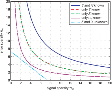
Figure 1: Recovery thresholds (15), (22), (26), (30), and eq:l1_final for $\mu_{a}=\mu_{b}=0$, and $\mu_{m}=1/\sqrt{64}$. Note that the curves for “only $\mathcal{E}$ known” and “only $\mathcal{X}$ known” are on top of each other.

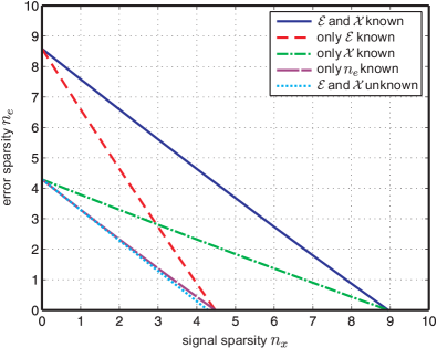
Figure 2: Recovery thresholds (15), (22), (26), (30), and eq:l1_final for $\mu_{a}=0.1258$, $\mu_{b}=0.1319$, and $\mu_{m}=0.1321$.

V-B The square-root bottleneck

The recovery thresholds presented in sec:main hold for all signal and noise realizations $\mathbf{x}$ and $\mathbf{e}$ and for all dictionary pairs (with given coherence parameters). However, as is well-known in the sparse-signal recovery literature, coherence-based recovery guarantees are—in contrast to RIC-based recovery guarantees—fundamentally limited by the so-called square-root bottleneck [48]. More specifically, in the noiseless case (i.e., for $\mathbf{e}=\mathbf{0}_{N_{b}}$), the threshold (4) states that recovery can be guaranteed only for up to $\sqrt{M}$ nonzero entries in $\mathbf{x}$. Put differently, for a fixed number of nonzero entries $n_{x}$ in $\mathbf{x}$, i.e., for a fixed sparsity level, the number of measurements $M$ required to recover $\mathbf{x}$ through (P0), BP, or OMP is on the order of $n_{x}^{2}$.

As in the classical sparse-signal recovery literature, the square-root bottleneck can be broken by performing a probabilistic analysis [48]. This line of work—albeit interesting—is outside the scope of the present paper and is further investigated in [49, 33, 50].

V-C Trade-off between $n_{x}$ and $n_{e}$

We next illustrate a trade-off between the sparsity levels of $\mathbf{x}$ and $\mathbf{e}$. Following the procedure outlined in [51, 12], we construct a dictionary $\mathbf{A}$ consisting of $A$ ONBs and a dictionary $\mathbf{B}$ consisting of $B$ ONBs such that $\mu_{a}=\mu_{b}=\mu_{m}=1/\sqrt{M}$, where $A+B\leq M+1$ with $M=p^{k}$, $p$ prime, and $k\in\mathbb{N}^{+}$. Now, let us assume that the error sparsity level scales according to $n_{e}=\alpha\sqrt{M}$ for some $0\leq\alpha\leq 1$. For the case where only $\mathcal{E}$ is known but $\mathcal{X}$ is unknown (Case II), we find from eq:P0uk_assump that any signal $\mathbf{x}$ with (order-wise) $(1-\alpha)\sqrt{M}/2$ non-zero entries (ignoring terms of order less than $\sqrt{M}$) can be reconstructed. Hence, there is a trade-off between the sparsity levels of $\mathbf{x}$ and $\mathbf{e}$ (here quantified through the parameter $\alpha$), and both sparsity levels scale with $\sqrt{M}$.

VI Numerical Results

We first report simulation results and compare them to the corresponding analytical results in the paper. We will find that even though the analytical thresholds are pessimistic in general, they do reflect the numerically observed recovery behavior correctly. In particular, we will see that the factor-of-two penalty discussed in sec:factortwoinguarantees can also be observed in the numerical results. We then demonstrate, through a simple inpainting example, that perfect signal recovery in the presence of sparse errors is possible even if the corruptions are significant (in terms of the $\ell_{2}$-norm of the sparse noise vector $\mathbf{e}$). In all numerical results, OMP is performed with a predetermined number of iterations [13, 24, 25], i.e., for Case II and Case IV, we set the number of iterations to $n_{x}$ and $n_{x}+n_{e}$, respectively. To implement BP, we employ SPGL1 [52, 53].

VI-A Impact of support-set knowledge on recovery thresholds

We first compare simulation results to the recovery thresholds (15), (22), (26), and eq:l1_final. For a given pair of dictionaries $\mathbf{A}$ and $\mathbf{B}$ we generate signal vectors $\mathbf{x}$ and error vectors $\mathbf{e}$ as follows: We first fix $n_{x}$ and $n_{e}$, then the support sets of the $n_{x}$-sparse vector $\mathbf{x}$ and the $n_{e}$-sparse vector $\mathbf{e}$ are chosen uniformly at random among all possible support sets of cardinality $n_{x}$ and $n_{e}$, respectively. Once the support sets have been chosen, we generate the nonzero entries of $\mathbf{x}$ and $\mathbf{e}$ by drawing from i.i.d. zero mean, unit variance Gaussian random variables. For each pair of support-set cardinalities $n_{x}$ and $n_{e}$, we perform 10 000 Monte-Carlo trials and declare success of recovery whenever the recovered vector $\hat{\mathbf{x}}$ satisfies

$$\mathopen{}\left\lVert\hat{\mathbf{x}}-\mathbf{x}\right\rVert_{2}<10^{-3}\mathopen{}\left\lVert\mathbf{x}\right\rVert_{2}.$$ (36)

We plot the 50% success-rate contour, i.e., the border between the region of pairs ($n_{x}$, $n_{e}$) for which (36) is satisfied in at least 50% of the trials and the region where (36) is satisfied in less than 50% of the trials. The recovered vector $\hat{}\mathbf{x}$ is obtained as follows:

• Case I: When $\mathcal{X}$ and $\mathcal{E}$ are both known, we perform recovery according to (14).

• Case II: When either only $\mathcal{E}$ or only $\mathcal{X}$ is known, we apply BP and OMP using the modified dictionary as detailed in thm:P1uk_equivalence and cor:P1_signal_known, respectively.

• Case IV: When neither $\mathcal{X}$ nor $\mathcal{E}$ is known, we apply BP and OMP to the concatenated dictionary $\mathbf{D}=[\,\mathbf{A}\,\,\mathbf{B}\,]$ as described in thm:l1_general.

Note that for Case III, i.e., the case where the cardinality $n_{e}$ of the support set $\mathcal{E}$ is known—as pointed out in sec:cardinalityKnown—we only have uniqueness results but no analytical recovery guarantees, neither for BP nor for greedy recovery algorithms that make use of the separate knowledge of $n_{x}$ or $n_{e}$ (whereas, e.g., standard OMP makes use of knowledge of $n_{x}+n_{e}$, rather than knowledge of $n_{x}$ and $n_{e}$ individually). This case is, therefore, not considered in the simulation results below.

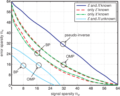
Figure 3: Impact of support-set knowledge on the 50% success-rate contour of OMP and BP for the Hadamard–identity pair.

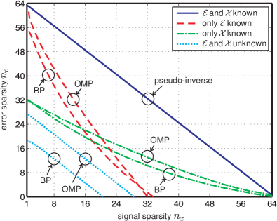
Figure 4: Impact of support-set knowledge on the 50% success-rate contour of OMP and BP performing recovery in pairs of approximate ETFs each of dimension $64\times 80$.

VI-A1 Recovery performance for the Hadamard–identity pair using BP and OMP

We take $M=64$, let $\mathbf{A}$ be the Hadamard ONB [54] and set $\mathbf{B}=\mathbf{I}_{M}$, which results in $\mu_{a}=\mu_{b}=0$ and $\mu_{m}=1/\sqrt{M}$. fig:pt_bpvsomp shows 50% success-rate contours, under different assumptions of support-set knowledge. For perfect knowledge of $\mathcal{X}$ and $\mathcal{E}$, we observe that the 50% success-rate contour is at about $n_{x}+n_{e}\approx M$, which is significantly better than the sufficient condition $n_{x}n_{e}<M$ (guaranteeing perfect recovery) provided in (15). When either only $\mathcal{X}$ or only $\mathcal{E}$ is known, the recovery performance is essentially independent of whether $\mathcal{X}$ or $\mathcal{E}$ is known. This is also reflected by the analytical thresholds (22) and (26) when evaluated for $\mu_{a}=\mu_{b}=0$ (see also fig:th_th_ONB). Furthermore, OMP is seen to outperform BP. When neither $\mathcal{X}$ nor $\mathcal{E}$ is known, OMP again outperforms BP.

It is interesting to see that the factor-of-two penalty discussed in sec:factortwoinguarantees is reflected in fig:pt_bpvsomp (for $n_{x}=n_{e}$) between Cases I and II. Specifically, we can observe that for full support-set knowledge (Case I) the 50% success-rate is achieved at $n_{x}=n_{e}\approx 31$. If either $\mathcal{X}$ or $\mathcal{E}$ only is known (Case II), OMP achieves 50% success-rate at $n_{x}=n_{e}\approx 23$, demonstrating a factor-of-two penalty since $31\cdot 31\approx 23\cdot 23\cdot 2$. Note that the results from BP in fig:pt_bpvsomp do not seem to reflect the factor-of-two penalty. For lack of an efficient recovery algorithm (making use of knowledge of $n_{e}$) we do not show numerical results for Case III.

VI-A2 Impact of $\mu_{a},\mu_{b}>0$

We take $M=64$ and generate the dictionaries $\mathbf{A}$ and $\mathbf{B}$ as follows. Using the alternating projection method described in [56], we generate an approximate equiangular tight frame (ETF) for $\mathbb{R}^{M}$ consisting of $160$ columns. We split this frame into two sets of $80$ elements (columns) each and organize them in the matrices $\mathbf{A}$ and $\mathbf{B}$ such that the corresponding coherence parameters are given by $\mu_{a}\approx 0.1258$, $\mu_{b}\approx 0.1319$, and $\mu_{m}\approx 0.1321$. fig:pt_orthvsrand_OMP shows the 50% success-rate contour under four different assumptions of support-set knowledge. In the case where either only $\mathcal{X}$ or only $\mathcal{E}$ is known and in the case where $\mathcal{X}$ and $\mathcal{E}$ are unknown, we use OMP and BP for recovery. It is interesting to note that the graphs for the cases where only $\mathcal{X}$ or only $\mathcal{E}$ are known, are symmetric with respect to the line $n_{x}=n_{e}$. This symmetry is also reflected in the analytical thresholds (22) and (26) (see also fig:th_th_sym and the discussion in sec:factortwoinguarantees).

We finally note that in all cases considered above, the numerical results show that recovery is possible for significantly higher sparsity levels $n_{x}$ and $n_{e}$ than indicated by the corresponding analytical thresholds (15), (22), (26), and eq:l1_final (see also Figs. 1 and 2). The underlying reasons are i) the deterministic nature of the results, i.e., the recovery guarantees in (15), (22), (26), and eq:l1_final are valid for all dictionary pairs (with given coherence parameters) and all signal and noise realizations (with given sparsity level), and ii) we plot the 50% success-rate contour, whereas the analytical results guarantee perfect recovery in 100% of the cases.

VI-B Inpainting example

In transform coding one is typically interested in maximally sparse representations of a given signal to be encoded [57]. In our setting, this would mean that the dictionary $\mathbf{A}$ should be chosen so that it leads to maximally sparse representations of a given family of signals. We next demonstrate, however, that in the presence of structured noise, the signal dictionary $\mathbf{A}$ should additionally be incoherent to the noise dictionary $\mathbf{B}$. This extra requirement can lead to very different criteria for designing transform bases (frames).

(a) Corrupted image
($\textsf{MSE}=-11.2$ dB)

(b) Recovery when $\mathcal{X}$ and $\mathcal{E}$ are known ($\textsf{MSE}=-184.6$ dB)

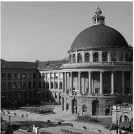
(c) Recovery when only $\mathcal{E}$ is known ($\textsf{MSE}=-113.3$ dB)

(d) Recovery for $\mathcal{X}$ and $\mathcal{E}$ unknown ($\textsf{MSE}=-13.0$ dB)

Figure 5: Recovery results using the DCT basis for the signal dictionary and the identity basis for the noise dictionary, for the cases where 6(b) $\mathcal{X}$ and $\mathcal{E}$ are known, 6(c) only $\mathcal{E}$ is known, and 6(d) no support-set knowledge is available. (Picture origin: ETH Zürich/Esther Ramseier).

(a) Corrupted image
($\textsf{MSE}=-11.2$ dB)

(b) Recovery when $\mathcal{X}$ and $\mathcal{E}$ are known ($\textsf{MSE}=-27.1$ dB)

(c) Recovery when only $\mathcal{E}$ is known ($\textsf{MSE}=-27.1$ dB)

(d) Recovery for $\mathcal{X}$ and $\mathcal{E}$ unknown ($\textsf{MSE}=-12.0$ dB)

Figure 6: Recovery results for the signal dictionary given by the Haar wavelet basis and the noise dictionary given by the identity basis, for the cases where 6(b) both $\mathcal{X}$ and $\mathcal{E}$ are known, 6(c) only $\mathcal{E}$ is known, and 6(d) no support-set knowledge is available. (Picture origin: ETH Zürich/Esther Ramseier).

To illustrate this point, and to show that perfect recovery can be guaranteed even when the $\ell_{2}$-norm of the noise term $\mathbf{B}\mathbf{e}$ is large, we consider the recovery of a sparsely corrupted 512$\times$512-pixel grayscale image of the main building of ETH Zurich. The dictionary $\mathbf{A}$ is taken to be either the two-dimensional discrete cosine transform (DCT) or the Haar wavelet decomposed on three octaves [58]. We first “sparsify” the image by retaining the 15% largest entries of the image’s representation $\mathbf{x}$ in $\mathbf{A}$. We then corrupt (by overwriting with text) 18.8% of the pixels in the sparsified image by setting them to the brightest grayscale value; this means that the errors are sparse in $\mathbf{B}=\mathbf{I}_{M}$ and that the noise is structured but may have large $\ell_{2}$-norm. Image recovery is performed according to eq:recoveryifeverythingisknown if $\mathcal{X}$ and $\mathcal{E}$ are known. (Note, however, that knowledge of $\mathcal{X}$ is usually not available in inpainting applications.) We use BP when only $\mathcal{E}$ is known and when neither $\mathcal{X}$ nor $\mathcal{E}$ are known. The recovery results are evaluated by computing the mean-square error (MSE) between the sparsified image and its recovered version.

Figs. 5 and 6 show the corresponding results. As expected, the MSE increases as the amount of knowledge about the support sets decreases. More interestingly, we note that even though Haar wavelets often yield a smaller approximation error in classical transform coding compared to the DCT, here the wavelet transform performs worse than the DCT. This behavior is due to the fact that sparsity is not the only factor determining the performance of a transform coding basis (or frame) in the presence of structured noise. Rather the mutual coherence between the dictionary used to represent the signal and that used to represent the structured noise becomes highly relevant. Specifically, in the example at hand, we have $\mu_{m}=1/2$ for the Haar-wavelet and the identity basis, and $\mu_{m}\approx 0.004$ for the DCT and the identity basis. The dependence of the analytical thresholds (15), (22), (26), (30), and eq:l1_final on the mutual coherence $\mu_{m}$ explains the performance difference between the Haar wavelet basis and the DCT basis. An intuitive explanation for this behavior is as follows: The Haar-wavelet basis contains only four non-zero entries in the columns associated to fine scales, which is reflected in the high mutual coherence (i.e., $\mu_{m}=1/2$) between the Haar-wavelet basis and the identity basis. Thus, when projecting onto the orthogonal complement of $(\mathbf{I}_{M})_{\mathcal{E}}$, it is likely that all non-zero entries of such columns are deleted, resulting in columns of all zeros. Recovery of the corresponding non-zero entries of $\mathbf{x}$ is thus not possible. In summary, we see that the choice of the transform basis (frame) for a sparsely corrupted signal should not only aim at sparsifying the signal as much as possible but should also take into account the mutual coherence between the transform basis (frame) and the noise sparsity basis (frame).

VII Conclusion

The setup considered in this paper, in its generality, appears to be new and a number of interesting extensions are possible. In particular, developing (coherence-based) recovery guarantees for greedy algorithms such as CoSaMP [41] or subspace pursuit [42] for all cases studied in the paper are interesting open problems. Note that probabilistic recovery guarantees for the case where nothing is known about the signal and noise support sets (i.e., Case IV) readily follow from the results in [33]. Probabilistic recovery guarantees for the other cases studied in this paper are in preparation [50]. Furthermore, an extension of the results in this paper that accounts for measurement noise (in addition to sparse noise) and applies to approximately sparse signals can be found in [59].

Appendix A Proof of thm:P1_bothknown

We prove the full (column-)rank property of $\mathbf{D}_{\mathcal{X},\mathcal{E}}$ by showing that under (15) there is a unique pair $(\mathbf{x},\mathbf{e})$ with $\textrm{supp}(\mathbf{x})=\mathcal{X}$ and $\textrm{supp}(\mathbf{e})=\mathcal{E}$ satisfying $\mathbf{z}=\mathbf{A}\mathbf{x}+\mathbf{B}\mathbf{e}$. Assume that there exists an alternative pair $(\mathbf{x}^{\prime},\mathbf{e}^{\prime})$ such that $\mathbf{z}=\mathbf{A}\mathbf{x}^{\prime}+\mathbf{B}\mathbf{e}^{\prime}$ with $\textrm{supp}(\mathbf{x}^{\prime})\subseteq\mathcal{X}$ and $\textrm{supp}(\mathbf{e}^{\prime})\subseteq\mathcal{E}$ (i.e., the support sets of $\mathbf{x}^{\prime}$ and $\mathbf{e}^{\prime}$ are contained in $\mathcal{X}$ and $\mathcal{E}$, respectively). This would then imply that

$$\mathbf{A}\mathbf{x}+\mathbf{B}\mathbf{e}=\mathbf{A}\mathbf{x}^{\prime}+\mathbf{B}\mathbf{e}^{\prime}$$

and thus

$$\mathbf{A}(\mathbf{x}-\mathbf{x}^{\prime})=\mathbf{B}(\mathbf{e}^{\prime}-\mathbf{e}).$$

Since both $\mathbf{x}$ and $\mathbf{x}^{\prime}$ have support in $\mathcal{X}$ it follows that $\mathbf{x}-\mathbf{x}^{\prime}$ also has support in $\mathcal{X}$, which implies $\mathopen{}\left\lVert\mathbf{x}-\mathbf{x}^{\prime}\right\rVert_{0}\leq n_{x}$. Similarly, we get $\mathopen{}\left\lVert\mathbf{e}^{\prime}-\mathbf{e}\right\rVert_{0}\leq n_{e}$. Defining $\mathbf{p}=\mathbf{x}-\mathbf{x}^{\prime}$ and $\mathcal{P}=\textrm{supp}(\mathbf{x}-\mathbf{x}^{\prime})\subseteq\mathcal{X}$, and, similarly, $\mathbf{q}=\mathbf{e}^{\prime}-\mathbf{e}$ and $\mathcal{Q}=\textrm{supp}(\mathbf{e}^{\prime}-\mathbf{e})\subseteq\mathcal{E}$, we obtain the following chain of inequalities:

$$n_{x}n_{e} \geq\mathopen{}\left\lVert\mathbf{p}\right\rVert_{0}\mathopen{}\left\lVert\mathbf{q}\right\rVert_{0}=\mathopen{}\left\lvert\mathcal{P}\right\rvert\mathopen{}\left\lvert\mathcal{Q}\right\rvert$$

$$\geq\frac{\mathopen{}\left[1-\mu_{a}(\mathopen{}\left\lvert\mathcal{P}\right\rvert-1)\right]^{+}\mathopen{}\left[1-\mu_{b}(\mathopen{}\left\lvert\mathcal{Q}\right\rvert-1)\right]^{+}}{\mu_{m}^{2}}$$ (37)

$$\geq\frac{\mathopen{}\left[1-\mu_{a}(n_{x}-1)\right]^{+}\mathopen{}\left[1-\mu_{b}(n_{e}-1)\right]^{+}}{\mu_{m}^{2}}=f(n_{x},n_{e})$$ (38)

where (37) follows by applying the uncertainty relation in thm:uncertainty (with $\epsilon_{\mathcal{P}}=\epsilon_{\mathcal{Q}}=0$ since both $\mathbf{p}$ and $\mathbf{q}$ are perfectly concentrated to $\mathcal{P}$ and $\mathcal{Q}$, respectively) and (38) is a consequence of $\mathopen{}\left\lvert\mathcal{P}\right\rvert\leq n_{x}$ and $\mathopen{}\left\lvert\mathcal{Q}\right\rvert\leq n_{e}$. Obviously, (38) contradicts the assumption in (15), which completes the proof.

Appendix B Proof of thm:P0_uk

We begin by proving that $\mathbf{x}$ is the unique solution of $(\textrm{P0},\mathcal{E})$ applied to $\mathbf{z}=\mathbf{A}\mathbf{x}+\mathbf{B}\mathbf{e}$. Assume that there exists an alternative vector $\mathbf{x}^{\prime}$ that satisfies $\mathbf{A}\mathbf{x}^{\prime}\in(\{\mathbf{z}\}+\mathcal{R}(\mathbf{B}_{\mathcal{E}}))$ with $\mathopen{}\left\lVert\mathbf{x}^{\prime}\right\rVert_{0}\leq n_{x}$. This would imply the existence of a vector $\mathbf{e}^{\prime}$ with $\textrm{supp}(\mathbf{e}^{\prime})\subseteq\mathcal{E}$, such that

$$\mathbf{A}\mathbf{x}+\mathbf{B}\mathbf{e}=\mathbf{A}\mathbf{x}^{\prime}+\mathbf{B}\mathbf{e}^{\prime}$$

and hence

$$\mathbf{A}(\mathbf{x}-\mathbf{x}^{\prime})=\mathbf{B}(\mathbf{e}^{\prime}-\mathbf{e}).$$

Since $\textrm{supp}(\mathbf{e})=\mathcal{E}$ and $\textrm{supp}(\mathbf{e}^{\prime})\subseteq\mathcal{E}$, we have $\textrm{supp}(\mathbf{e}^{\prime}-\mathbf{e})\subseteq\mathcal{E}$ and hence $\mathopen{}\left\lVert\mathbf{e}^{\prime}-\mathbf{e}\right\rVert_{0}\leq n_{e}$. Furthermore, since both $\mathbf{x}$ and $\mathbf{x}^{\prime}$ have at most $n_{x}$ nonzero entries, we have $\mathopen{}\left\lVert\mathbf{x}-\mathbf{x}^{\prime}\right\rVert_{0}\leq 2n_{x}$. Defining $\mathbf{p}=\mathbf{x}-\mathbf{x}^{\prime}$ and $\mathcal{P}=\textrm{supp}(\mathbf{x}-\mathbf{x}^{\prime})$, and, similarly, $\mathbf{q}=\mathbf{e}^{\prime}-\mathbf{e}$ and $\mathcal{Q}=\textrm{supp}(\mathbf{e}^{\prime}-\mathbf{e})\subseteq\mathcal{E}$, we obtain the following chain of inequalities

$$2n_{x}n_{e} \geq\mathopen{}\left\lVert\mathbf{p}\right\rVert_{0}\mathopen{}\left\lVert\mathbf{q}\right\rVert_{0}=\mathopen{}\left\lvert\mathcal{P}\right\rvert\mathopen{}\left\lvert\mathcal{Q}\right\rvert$$

$$\geq\frac{\mathopen{}\left[1-\mu_{a}(\mathopen{}\left\lvert\mathcal{P}\right\rvert\!-\!1)\right]^{+}\mathopen{}\left[1-\mu_{b}(\mathopen{}\left\lvert\mathcal{Q}\right\rvert\!-\!1)\right]^{+}}{\mu_{m}^{2}}$$ (39)

$$\geq\frac{\mathopen{}\left[1-\mu_{a}(2n_{x}\!-\!1)\right]^{+}\mathopen{}\left[1-\mu_{b}(n_{e}\!-\!1)\right]^{+}}{\mu_{m}^{2}}=f(2n_{x},n_{e})$$ (40)

where (39) follows by applying the uncertainty relation in thm:uncertainty (with $\epsilon_{\mathcal{P}}=\epsilon_{\mathcal{Q}}=0$ since both $\mathbf{p}$ and $\mathbf{q}$ are perfectly concentrated to $\mathcal{P}$ and $\mathcal{Q}$, respectively) and (40) is a consequence of $\mathopen{}\left\lvert\mathcal{P}\right\rvert\leq 2n_{x}$ and $\mathopen{}\left\lvert\mathcal{Q}\right\rvert\leq n_{e}$. Obviously, (40) contradicts the assumption in (22), which concludes the first part of the proof.

We next prove that $\mathbf{x}$ is also the unique solution of $(\textrm{BP},\mathcal{E})$ applied to $\mathbf{z}=\mathbf{A}\mathbf{x}+\mathbf{B}\mathbf{e}$. Assume that there exists an alternative vector $\mathbf{x}^{\prime}$ that satisfies $\mathbf{A}\mathbf{x}^{\prime}\in(\{\mathbf{z}\}+\mathcal{R}(\mathbf{B}_{\mathcal{E}}))$ with $\mathopen{}\left\lVert\mathbf{x}^{\prime}\right\rVert_{1}\leq\mathopen{}\left\lVert\mathbf{x}\right\rVert_{1}$. This would imply the existence of a vector $\mathbf{e}^{\prime}$ with $\textrm{supp}(\mathbf{e}^{\prime})\subseteq\mathcal{E}$, such that

$$\mathbf{A}\mathbf{x}+\mathbf{B}\mathbf{e}=\mathbf{A}\mathbf{x}^{\prime}+\mathbf{B}\mathbf{e}^{\prime}$$

and hence

$$\mathbf{A}(\mathbf{x}-\mathbf{x}^{\prime})=\mathbf{B}(\mathbf{e}^{\prime}-\mathbf{e}).$$

Defining $\mathbf{p}=\mathbf{x}-\mathbf{x}^{\prime}$, we obtain the following lower bound for the $\ell_{1}$-norm of $\mathbf{x}^{\prime}$

$$\mathopen{}\left\lVert\mathbf{x}^{\prime}\right\rVert_{1}=\mathopen{}\left\lVert\mathbf{x}-\mathbf{p}\right\rVert_{1} =\mathopen{}\left\lVert\mathbf{P}_{\mathcal{X}}(\mathbf{x}-\mathbf{p})\right\rVert_{1}+\mathopen{}\left\lVert\mathbf{P}_{\mathcal{X}^{c}}\mathbf{p}\right\rVert_{1}$$

$$\geq\mathopen{}\left\lVert\mathbf{P}_{\mathcal{X}}\mathbf{x}\right\rVert_{1}-\mathopen{}\left\lVert\mathbf{P}_{\mathcal{X}}\mathbf{p}\right\rVert_{1}+\mathopen{}\left\lVert\mathbf{P}_{\mathcal{X}^{c}}\mathbf{p}\right\rVert_{1}$$ (41)

$$=\mathopen{}\left\lVert\mathbf{x}\right\rVert_{1}-\mathopen{}\left\lVert\mathbf{P}_{\mathcal{X}}\mathbf{p}\right\rVert_{1}+\mathopen{}\left\lVert\mathbf{P}_{\mathcal{X}^{c}}\mathbf{p}\right\rVert_{1}$$

where (41) is a consequence of the reverse triangle inequality. Now, the $\ell_{1}$-norm of $\mathbf{x}^{\prime}$ can be smaller than or equal to that of $\mathbf{x}$ only if $\mathopen{}\left\lVert\mathbf{P}_{\mathcal{X}}\mathbf{p}\right\rVert_{1}\geq\mathopen{}\left\lVert\mathbf{P}_{\mathcal{X}^{c}}\mathbf{p}\right\rVert_{1}$. This would then imply that the difference vector $\mathbf{p}$ needs to be at least 50%-concentrated to the set $\mathcal{P}=\mathcal{X}$ (of cardinality $n_{x}$), i.e., we require that $\epsilon_{\mathcal{P}}\leq 0.5$. Defining $\mathbf{q}=\mathbf{e}^{\prime}-\mathbf{e}$ and $\mathcal{Q}=\textrm{supp}(\mathbf{e}^{\prime}-\mathbf{e})$, and noting that $\textrm{supp}(\mathbf{e})=\mathcal{E}$ and $\textrm{supp}(\mathbf{e}^{\prime})\subseteq\mathcal{E}$, it follows that $\mathopen{}\left\lvert\mathcal{Q}\right\rvert\leq n_{e}$. This leads to the following chain of inequalities:

$$n_{x}\,n_{e} \geq\mathopen{}\left\lvert\mathcal{P}\right\rvert\mathopen{}\left\lvert\mathcal{Q}\right\rvert$$

$$\geq\frac{\mathopen{}\left[(1+\mu_{a})(1-\epsilon_{\mathcal{P}})-\mathopen{}\left\lvert\mathcal{P}\right\rvert\mu_{a}\right]^{+}\mathopen{}\left[1-\mu_{b}\left(\mathopen{}\left\lvert\mathcal{Q}\right\rvert-1\right)\right]^{+}}{\mu_{m}^{2}}$$ (42)

$$\geq\frac{1}{2}\,\frac{\mathopen{}\left[1-\mu_{a}(2n_{x}-1)\right]^{+}\mathopen{}\left[1-\mu_{b}(n_{e}-1)\right]^{+}}{\mu_{m}^{2}}$$ (43)

where (42) follows from the uncertainty relation in thm:uncertainty applied to the difference vectors $\mathbf{p}$ and $\mathbf{q}$ (with $\epsilon_{\mathcal{P}}\leq 0.5$ since $\mathbf{p}$ is at least 50%-concentrated to $\mathcal{P}$ and $\epsilon_{\mathcal{Q}}=0$ since $\mathbf{q}$ is perfectly concentrated to $\mathcal{Q}$) and (43) is a consequence of $\mathopen{}\left\lvert\mathcal{P}\right\rvert=n_{x}$ and $\mathopen{}\left\lvert\mathcal{Q}\right\rvert\leq n_{e}$. Rewriting (43), we obtain

$$2n_{x}n_{e}\geq\frac{\mathopen{}\left[1\!-\!\mu_{a}(2n_{x}\!-\!1)\right]^{+}\mathopen{}\left[1\!-\!\mu_{b}(n_{e}\!-\!1)\right]^{+}}{\mu_{m}^{2}}=f(2n_{x},n_{e}).$$ (44)

Since (44) contradicts the assumption in (22), this proves that $\mathbf{x}$ is the unique solution of $(\textrm{BP},\mathcal{E})$ applied to $\mathbf{z}=\mathbf{A}\mathbf{x}+\mathbf{B}\mathbf{e}$.

Appendix C Proof of thm:P1uk_equivalence

We first show that condition (22) ensures that the columns of $\mathbf{B}_{\mathcal{E}}$ are linearly independent. Then, we establish that $\mathopen{}\left\lVert\mathbf{R}_{\mathcal{E}}\mathbf{a}_{\ell}\right\rVert_{2}>0$ for $\ell=1,\ldots,{N_{a}}$. Finally, we show that the unique solution of (P0), BP, and OMP applied to $\hat{}\mathbf{z}=\mathbf{R}_{\mathcal{E}}\mathbf{A}\mathbf{\Delta}\hat{\mathbf{x}}$ is given by $\hat{\mathbf{x}}=\mathbf{\Delta}^{-1}\mathbf{x}$.

C-A The columns of $\mathbf{B}_{\mathcal{E}}$ are linearly independent

Condition (22) can only be satisfied if $\mathopen{}\left[1\!-\!\mu_{b}(n_{e}\!-\!1)\right]^{+}>0$, which implies that $n_{e}<1+1/\mu_{b}$. It was shown in [11, 12, 13] that for a dictionary $\mathbf{B}$ with coherence $\mu_{b}$ no fewer than $1+1/\mu_{b}$ columns of $\mathbf{B}$ can be linearly dependent. Hence, the $n_{e}$ columns of $\mathbf{B}_{\mathcal{E}}$ must be linearly independent.

C-B $\mathopen{}\left\lVert\mathbf{R}_{\mathcal{E}}\mathbf{a}_{\ell}\right\rVert_{2}>0$ for $\ell=1,\ldots,{N_{a}}$

We have to verify that condition (22) implies $\mathopen{}\left\lVert\mathbf{R}_{\mathcal{E}}\mathbf{a}_{\ell}\right\rVert_{2}>0$ for $\ell=1,\ldots,{N_{a}}$. Since $\mathbf{R}_{\mathcal{E}}$ is a projector and, therefore, Hermitian and idempotent, it follows that

$$\mathopen{}\left\lVert\mathbf{R}_{\mathcal{E}}\mathbf{a}_{\ell}\right\rVert_{2}^{2} =\mathbf{a}_{\ell}^{H}\mathbf{R}_{\mathcal{E}}\mathbf{a}_{\ell}$$ (45)

$$=\mathopen{}\left\lvert\mathbf{a}_{\ell}^{H}\mathbf{R}_{\mathcal{E}}\mathbf{a}_{\ell}\right\rvert$$

$$\geq 1-\underbrace{\mathopen{}\left\lvert\mathbf{a}_{\ell}^{H}\mathbf{B}_{\mathcal{E}}\left(\mathbf{B}^{H}_{\mathcal{E}}\mathbf{B}_{\mathcal{E}}\right)^{-1}\mathbf{B}^{H}_{\mathcal{E}}\mathbf{a}_{\ell}\right\rvert}_{\triangleq\,C_{1}}$$ (46)

where (45) is a consequence of $\mathbf{R}_{\mathcal{E}}^{H}\mathbf{R}_{\mathcal{E}}=\mathbf{R}_{\mathcal{E}}$, and (46) follows from the reverse triangle inequality and $\mathopen{}\left\lVert\mathbf{a}_{\ell}\right\rVert_{2}=1$, $\ell=1,\ldots,{N_{a}}$. Next, we derive an upper bound on $C_{1}$ according to

$$C_{1} \leq\lambda_{\text{max}}\mathopen{}\left(\!\left(\mathbf{B}^{H}_{\mathcal{E}}\mathbf{B}_{\mathcal{E}}\right)^{\!-1}\right)\mathopen{}\left\lVert\mathbf{B}^{H}_{\mathcal{E}}\mathbf{a}_{\ell}\right\rVert_{2}^{2}$$ (47)

$$\leq\lambda^{-1}_{\text{min}}\!\left(\mathbf{B}^{H}_{\mathcal{E}}\mathbf{B}_{\mathcal{E}}\right)n_{e}\,\mu_{m}^{2}$$ (48)

where (47) follows from the Rayleigh-Ritz theorem [60, Thm. 4.2.2] and (48) results from

$$\mathopen{}\left\lVert\mathbf{B}_{\mathcal{E}}^{H}\mathbf{a}_{\ell}\right\rVert_{2}^{2}=\sum_{i\in\mathcal{E}}\,\mathopen{}\left\lvert\mathbf{b}^{H}_{i}\mathbf{a}_{\ell}\right\rvert^{2}\leq n_{e}\,\mu_{m}^{2}.$$

Next, applying Geršgorin’s disc theorem [60, Theorem 6.1.1], we arrive at

$$\lambda_{\text{min}}\mathopen{}\left(\mathbf{B}^{H}_{\mathcal{E}}\mathbf{B}_{\mathcal{E}}\right)\geq\mathopen{}\left[1-\mu_{b}(n_{e}-1)\right]^{+}.$$ (49)

Combining eq:projectedcolumnslower1, eq:equivalence_bound2, and eq:equivalence_bound3 leads to the following lower bound on $\mathopen{}\left\lVert\mathbf{R}_{\mathcal{E}}\mathbf{a}_{\ell}\right\rVert_{2}^{2}$:

$$\mathopen{}\left\lVert\mathbf{R}_{\mathcal{E}}\mathbf{a}_{\ell}\right\rVert_{2}^{2}\geq 1-\frac{n_{e}\,\mu_{m}^{2}}{\mathopen{}\left[1-\mu_{b}(n_{e}-1)\right]^{+}}.$$ (50)

Note that if condition (22) holds for $n_{x}\geq 1$, it follows that $n_{e}\,\mu_{m}^{2}<\mathopen{}\left[1-\mu_{b}(n_{e}-1)\right]^{+}$ and hence the RHS of (50) is strictly positive. This ensures that $\mathbf{\Delta}$ defines a one-to-one mapping. We next show that, moreover, condition (22) ensures that for every vector $\mathbf{x}^{\prime}\in\mathbb{C}^{N_{a}}$ satisfying $\mathopen{}\left\lVert\mathbf{x}^{\prime}\right\rVert_{0}\leq 2n_{x}$, $\mathbf{A}\mathbf{x}^{\prime}$ has a nonzero component that is orthogonal to $\mathcal{R}(\mathbf{B}_{\mathcal{E}})$.

C-C Unique recovery through (P0), BP, and OMP

We now need to verify that (P0), BP, and OMP (applied to $\hat{}\mathbf{z}=\mathbf{R}_{\mathcal{E}}\mathbf{A}\mathbf{\Delta}\hat{}\mathbf{x}$) recover the vector $\hat{\mathbf{x}}=\mathbf{\Delta}^{\!-1}\mathbf{x}$ provided that (22) is satisfied. This will be accomplished by deriving an upper bound on the coherence $\mu(\mathbf{R}_{\mathcal{E}}\mathbf{A}\mathbf{\Delta})$ of the modified dictionary $\mathbf{R}_{\mathcal{E}}\mathbf{A}\mathbf{\Delta}$, which, via the well-known coherence-based recovery guarantee [11, 12, 13]

$$n_{x}<\frac{1}{2}\Big{(}1+\mu_{d}(\mathbf{R}_{\mathcal{E}}\mathbf{A}\mathbf{\Delta})^{-1}\Big{)}$$ (51)

leads to a recovery threshold guaranteeing perfect recovery of $\hat{\mathbf{x}}$. This threshold is then shown to coincide with (22). More specifically, the well-known sparsity threshold in (4) guarantees that the unique solution of (P0) applied to $\hat{}\mathbf{z}=\mathbf{R}_{\mathcal{E}}\mathbf{A}\mathbf{\Delta}\hat{}\mathbf{x}$ is given by $\hat{}\mathbf{x}$, and, furthermore, that this unique solution can be obtained through BP and OMP if eq:modifiedDictRecovery holds. It is important to note that $\mathopen{}\left\lVert\hat{\mathbf{x}}\right\rVert_{0}=\mathopen{}\left\lVert\mathbf{x}\right\rVert_{0}=n_{x}$. With

$$[\mathbf{\Delta}]_{\ell,\ell}=\frac{1}{\mathopen{}\left\lVert\mathbf{R}_{\mathcal{E}}\mathbf{a}_{\ell}\right\rVert_{2}},\quad\ell=1,\ldots,N_{a}$$

we obtain

$$\mu(\mathbf{R}_{\mathcal{E}}\mathbf{A}\mathbf{\Delta})=\max_{r,\ell,\ell\neq r}\frac{\mathopen{}\left\lvert\mathbf{a}_{r}^{H}\mathbf{R}_{\mathcal{E}}^{H}\mathbf{R}_{\mathcal{E}}\mathbf{a}_{\ell}\right\rvert}{\mathopen{}\left\lVert\mathbf{R}_{\mathcal{E}}\mathbf{a}_{r}\right\rVert_{2}\mathopen{}\left\lVert\mathbf{R}_{\mathcal{E}}\mathbf{a}_{\ell}\right\rVert_{2}}.$$ (52)

Next, we upper-bound the RHS of eq:equivalence_1 by upper-bounding its numerator and lower-bounding its denominator. For the numerator we have

$$\mathopen{}\left\lvert\mathbf{a}_{r}^{H}\mathbf{R}_{\mathcal{E}}^{H}\mathbf{R}_{\mathcal{E}}\mathbf{a}_{\ell}\right\rvert =\mathopen{}\left\lvert\mathbf{a}_{r}^{H}\mathbf{R}_{\mathcal{E}}\mathbf{a}_{\ell}\right\rvert$$ (53)

$$\leq\mathopen{}\left\lvert\mathbf{a}_{r}^{H}\mathbf{a}_{\ell}\right\rvert+\mathopen{}\left\lvert\mathbf{a}_{r}^{H}\mathbf{B}_{\mathcal{E}}\mathbf{B}^{\dagger}_{\mathcal{E}}\mathbf{a}_{\ell}\right\rvert$$ (54)

$$\leq\mu_{a}+\underbrace{\mathopen{}\left\lvert\mathbf{a}_{r}^{H}\mathbf{B}_{\mathcal{E}}\left(\mathbf{B}^{H}_{\mathcal{E}}\mathbf{B}_{\mathcal{E}}\right)^{-1}\mathbf{B}^{H}_{\mathcal{E}}\mathbf{a}_{\ell}\right\rvert}_{\triangleq\,C_{2}}$$ (55)

where (53) follows from $\mathbf{R}_{\mathcal{E}}^{H}\mathbf{R}_{\mathcal{E}}=\mathbf{R}_{\mathcal{E}}$, (54) is obtained through the triangle inequality, and (55) follows from $\mathopen{}\left\lvert\mathbf{a}_{r}^{H}\mathbf{a}_{\ell}\right\rvert\leq\mu_{a}$. Next, we derive an upper bound on $C_{2}$ according to

$$C_{2} \leq\mathopen{}\left\lVert\mathbf{B}^{H}_{\mathcal{E}}\mathbf{a}_{r}\right\rVert_{2}\mathopen{}\left\lVert\left(\mathbf{B}^{H}_{\mathcal{E}}\mathbf{B}_{\mathcal{E}}\right)^{-1}\mathbf{B}^{H}_{\mathcal{E}}\mathbf{a}_{\ell}\right\rVert_{2}$$ (56)

$$\leq\mathopen{}\left\lVert\mathbf{B}_{\mathcal{E}}^{H}\mathbf{a}_{r}\right\rVert_{2}\mathopen{}\left\lVert\left(\mathbf{B}^{H}_{\mathcal{E}}\mathbf{B}_{\mathcal{E}}\right)^{-1}\right\rVert\mathopen{}\left\lVert\mathbf{B}^{H}_{\mathcal{E}}\mathbf{a}_{\ell}\right\rVert_{2}$$ (57)

where (56) follows from the Cauchy-Schwarz inequality and (57) from the Rayleigh-Ritz theorem [60, Thm. 4.2.2]. Defining $i=\operatorname*{arg\;max}_{r}\mathopen{}\left\lVert\mathbf{B}_{\mathcal{E}}^{H}\mathbf{a}_{r}\right\rVert_{2}$, we further have

$$C_{2} \leq\mathopen{}\left\lVert\left(\mathbf{B}^{H}_{\mathcal{E}}\mathbf{B}_{\mathcal{E}}\right)^{-1}\right\rVert\mathopen{}\left\lVert\mathbf{B}_{\mathcal{E}}^{H}\mathbf{a}_{i}\right\rVert_{2}^{2}$$

$$=\lambda_{\text{max}}\mathopen{}\left(\left(\mathbf{B}^{H}_{\mathcal{E}}\mathbf{B}_{\mathcal{E}}\right)^{-1}\right)\mathopen{}\left\lVert\mathbf{B}_{\mathcal{E}}^{H}\mathbf{a}_{i}\right\rVert_{2}^{2}.$$

We obtain an upper bound on $C_{2}$ using the same steps that were used to bound $C_{1}$ in (47) – (49):

$$C_{2}\leq\frac{n_{e}\,\mu_{m}^{2}}{C_{b}}$$ (58)

where $C_{b}=\mathopen{}\left[1-\mu_{b}(n_{e}-1)\right]^{+}$. Combining eq:equivalence_bound1 and eq:C2bound leads to the following upper bound

$$\mathopen{}\left\lvert\mathbf{a}_{r}^{H}\mathbf{R}_{\mathcal{E}}^{H}\mathbf{R}_{\mathcal{E}}\mathbf{a}_{\ell}\right\rvert\leq\mu_{a}+\frac{n_{e}\,\mu_{m}^{2}}{C_{b}}.$$ (59)

Next, we derive a lower bound on the denominator on the RHS of (52). To this end, we set $j=\operatorname*{arg\;min}_{r}\mathopen{}\left\lVert\mathbf{R}_{\mathcal{E}}\mathbf{a}_{r}\right\rVert_{2}$ and note that

$$\mathopen{}\left\lVert\mathbf{R}_{\mathcal{E}}\mathbf{a}_{r}\right\rVert_{2}\mathopen{}\left\lVert\mathbf{R}_{\mathcal{E}}\mathbf{a}_{\ell}\right\rVert_{2} \geq\mathopen{}\left\lVert\mathbf{R}_{\mathcal{E}}\mathbf{a}_{j}\right\rVert_{2}^{2}$$

$$\geq 1-\frac{n_{e}\,\mu_{m}^{2}}{C_{b}}$$ (60)

where (60) follows from (50). Finally, combining (59) and (60) we arrive at

$$\mu(\mathbf{R}_{\mathcal{E}}\mathbf{A}\mathbf{\Delta})\leq\frac{\mu_{a}C_{b}+n_{e}\,\mu_{m}^{2}}{C_{b}-n_{e}\,\mu_{m}^{2}}.$$ (61)

Inserting (61) into the recovery threshold in (51), we obtain the following threshold guaranteeing recovery of $\hat{}\mathbf{x}$ from $\hat{\mathbf{z}}=\mathbf{R}_{\mathcal{E}}\mathbf{A}\mathbf{\Delta}\hat{\mathbf{x}}$ through $(\textrm{P0})$, BP, and OMP:

$$n_{x}<\frac{1}{2}\left(\frac{C_{b}(1+\mu_{a})}{\mu_{a}C_{b}+n_{e}\,\mu_{m}^{2}}\right).$$ (62)

Since $2n_{x}n_{e}\,\mu_{m}^{2}\geq 0$, we can transform (62) into

$$2n_{x}n_{e}\,\mu_{m}^{2} <C_{b}\mathopen{}\left[1-\mu_{a}(2n_{x}-1)\right]^{+}$$

$$=\mathopen{}\left[1-\mu_{b}(n_{e}\,-1)\right]^{+}\mathopen{}\left[1-\mu_{a}(2n_{x}-1)\right]^{+}.$$ (63)

Rearranging terms in (63) finally yields

$$2n_{x}n_{e}<f(2n_{x},n_{e})$$

which proves that (22) guarantees recovery of the vector $\hat{\mathbf{x}}$ (and thus also of $\mathbf{x}=\mathbf{\Delta}\hat{\mathbf{x}}$) through (P0), BP, and OMP.

Appendix D Proof of thm:P0_nothingknown

Assume that there exists an alternative vector $\mathbf{x}^{\prime}$ that satisfies $\mathbf{A}\mathbf{x}^{\prime}\in(\{\mathbf{z}\}+\bigcup_{\mathcal{E}\in\mathscr{P}}\mathcal{R}(\mathbf{B}_{\mathcal{E}}))$ (with $\mathscr{P}=\wp_{n_{e}}(\{1,\ldots,{N_{b}}\})$) with $\mathopen{}\left\lVert\mathbf{x}^{\prime}\right\rVert_{0}\leq n_{x}$. This implies the existence of a vector $\mathbf{e}^{\prime}$ with $\mathopen{}\left\lVert\mathbf{e}^{\prime}\right\rVert_{0}\leq n_{e}$ such that

$$\mathbf{A}\mathbf{x}+\mathbf{B}\mathbf{e}=\mathbf{A}\mathbf{x}^{\prime}+\mathbf{B}\mathbf{e}^{\prime}$$

and therefore

$$\mathbf{A}(\mathbf{x}-\mathbf{x}^{\prime})=\mathbf{B}(\mathbf{e}^{\prime}-\mathbf{e}).$$

From $\mathopen{}\left\lVert\mathbf{x}\right\rVert_{0}=n_{x}$ and $\mathopen{}\left\lVert\mathbf{x}^{\prime}\right\rVert_{0}\leq n_{x}$ it follows that $\mathopen{}\left\lVert\mathbf{x}-\mathbf{x}^{\prime}\right\rVert_{0}\leq 2n_{x}$. Similarly, $\mathopen{}\left\lVert\mathbf{e}\right\rVert_{0}=n_{e}$ and $\mathopen{}\left\lVert\mathbf{e}^{\prime}\right\rVert_{0}\leq n_{e}$ imply $\mathopen{}\left\lVert\mathbf{e}^{\prime}-\mathbf{e}\right\rVert_{0}\leq 2n_{e}$. Defining $\mathbf{p}=\mathbf{x}-\mathbf{x}^{\prime}$ and $\mathcal{P}=\textrm{supp}(\mathbf{x}-\mathbf{x}^{\prime})$, and, similarly, $\mathbf{q}=\mathbf{e}^{\prime}-\mathbf{e}$ and $\mathcal{Q}=\textrm{supp}(\mathbf{e}^{\prime}-\mathbf{e})$, we arrive at

$$4n_{x}n_{e} \geq\mathopen{}\left\lVert\mathbf{p}\right\rVert_{0}\mathopen{}\left\lVert\mathbf{q}\right\rVert_{0}=\mathopen{}\left\lvert\mathcal{P}\right\rvert\mathopen{}\left\lvert\mathcal{Q}\right\rvert$$

$$\geq\frac{\mathopen{}\left[1\!-\!\mu_{a}(\mathopen{}\left\lvert\mathcal{P}\right\rvert\!-\!1)\right]^{+}\mathopen{}\left[1\!-\!\mu_{b}(\mathopen{}\left\lvert\mathcal{Q}\right\rvert\!-\!1)\right]^{+}}{\mu_{m}^{2}}$$ (64)

$$\geq\frac{\mathopen{}\left[1\!-\!\mu_{a}(2n_{x}\!-\!1)\right]^{+}\mathopen{}\left[1\!-\!\mu_{b}(2n_{e}\!-\!1)\right]^{+}}{\mu_{m}^{2}}\!=\!f(2n_{x},2n_{e})$$ (65)

where (64) follows from the uncertainty relation in thm:uncertainty applied to the difference vectors $\mathbf{p}$ and $\mathbf{q}$ (with $\epsilon_{\mathcal{P}}=\epsilon_{\mathcal{Q}}=0$ since both $\mathbf{p}$ and $\mathbf{q}$ are perfectly concentrated to $\mathcal{P}$ and $\mathcal{Q}$, respectively) and (65) is a consequence of $\mathopen{}\left\lvert\mathcal{P}\right\rvert\leq 2n_{x}$ and $\mathopen{}\left\lvert\mathcal{Q}\right\rvert\leq 2n_{e}$. Obviously, (65) is in contradiction to (30), which concludes the proof.

References

- [1] C. Studer, P. Kuppinger, G. Pope, and H. Bölcskei, “Sparse signal recovery from sparsely corrupted measurements,” in Proc. of IEEE Int. Symp. on Inf. Theory (ISIT), St. Petersburg, Russia, Aug. 2011, pp. 1422–1426.
- [2] J. S. Abel and J. O. Smith III, “Restoring a clipped signal,” in Proc. of IEEE Int. Conf. Acoust. Speech Sig. Proc., vol. 3, May 1991, pp. 1745–1748.
- [3] R. E. Carrillo, K. E. Barner, and T. C. Aysal, “Robust sampling and reconstruction methods for sparse signals in the presence of impulsive noise,” IEEE J. Sel. Topics Sig. Proc., vol. 4, no. 2, pp. 392–408, 2010.
- [4] C. Novak, C. Studer, A. Burg, and G. Matz, “The effect of unreliable LLR storage on the performance of MIMO-BICM,” in Proc. of 44th Asilomar Conf. on Signals, Systems, and Comput., Pacific Grove, CA, USA, Nov. 2010, pp. 736–740.
- [5] S. G. Mallat and G. Yu, “Super-resolution with sparse mixing estimators,” IEEE Trans. Image Proc., vol. 19, no. 11, pp. 2889–2900, Nov. 2010.
- [6] M. Elad and Y. Hel-Or, “Fast super-resolution reconstruction algorithm for pure translational motion and common space-invariant blur,” IEEE Trans. Image Proc., vol. 10, no. 8, pp. 1187–1193, Aug. 2001.
- [7] M. Bertalmio, G. Sapiro, V. Caselles, and C. Ballester, “Image inpainting,” in Proc. of 27th Ann. Conf. Comp. Graph. Int. Tech., 2000, pp. 417–424.
- [8] M. Aharon, M. Elad, and A. M. Bruckstein, “-SVD: An algorithm for designing overcomplete dictionaries for sparse representation,” IEEE Trans. Sig. Proc., vol. 54, no. 11, pp. 4311–4322, Nov. 2006.
- [9] M. Elad, J.-L. Starck, P. Querre, and D. L. Donoho, “Simultaneous cartoon and texture image inpainting using morphological component analysis (MCA),” Appl. Comput. Harmon. Anal., vol. 19, pp. 340–358, Nov. 2005.
- [10] D. L. Donoho and G. Kutyniok, “Microlocal analysis of the geometric separation problem,” Feb. 2010. [Online]. Available: http://arxiv.org/abs/1004.3006v1
- [11] D. L. Donoho and M. Elad, “Optimally sparse representation in general (nonorthogonal) dictionaries via minimization,” Proc. Natl. Acad. Sci. USA, vol. 100, no. 5, pp. 2197–2202, Mar. 2003.
- [12] R. Gribonval and M. Nielsen, “Sparse representations in unions of bases,” IEEE Trans. Inf. Theory, vol. 49, no. 12, pp. 3320–3325, Dec. 2003.
- [13] J. A. Tropp, “Greed is good: Algorithmic results for sparse approximation,” IEEE Trans. Inf. Theory, vol. 50, no. 10, pp. 2231–2242, Oct. 2004.
- [14] E. J. Candès and T. Tao, “Decoding by linear programming,” IEEE Trans. Inf. Theory, vol. 51, no. 12, pp. 4203–4215, Dec. 2005.
- [15] E. J. Candès, “The restricted isometry property and its implications for compressed sensing,” C. R. Acad. Sci. Paris, Ser. I, vol. 346, pp. 589–592, 2008.
- [16] T. T. Cai, L. Wang, and G. Xu, “Stable recovery of sparse signals and an oracle inequality,” IEEE Trans. Inf. Theory, vol. 56, no. 7, pp. 3516–3522, Jul. 2010.
- [17] D. L. Donoho, M. Elad, and V. N. Temlyakov, “Stable recovery of sparse overcomplete representations in the presence of noise,” IEEE Trans. Inf. Theory, vol. 52, no. 1, pp. 6–18, Jan. 2006.
- [18] J. J. Fuchs, “Recovery of exact sparse representations in the presence of bounded noise,” IEEE Trans. Inf. Theory, vol. 51, no. 10, pp. 3601–2608, Oct. 2005.
- [19] J. A. Tropp, “Just relax: Convex programming methods for identifying sparse signals in noise,” IEEE Trans. Inf. Theory, vol. 52, no. 3, pp. 1030–1051, Mar. 2006.
- [20] Z. Ben-Haim, Y. C. Eldar, and M. Elad, “Coherence-based performance guarantees for estimating a sparse vector under random noise,” IEEE Trans. Sig. Proc., vol. 58, no. 10, pp. 5030–5043, Oct. 2010.
- [21] S. S. Chen, D. L. Donoho, and M. A. Saunders, “Atomic decomposition by basis pursuit,” SIAM J. Sci. Comput., vol. 20, no. 1, pp. 33–61, 1998.
- [22] D. L. Donoho and X. Huo, “Uncertainty principles and ideal atomic decomposition,” IEEE Trans. Inf. Theory, vol. 47, no. 7, pp. 2845–2862, Nov. 2001.
- [23] M. Elad and A. M. Bruckstein, “A generalized uncertainty principle and sparse representation in pairs of bases,” IEEE Trans. Inf. Theory, vol. 48, no. 9, pp. 2558–2567, Sep. 2002.
- [24] Y. C. Pati, R. Rezaifar, and P. S. Krishnaprasad, “Orthogonal matching pursuit: Recursive function approximation with applications to wavelet decomposition,” in Proc. of 27th Asilomar Conf. on Signals, Systems, and Comput., Pacific Grove, CA, USA, Nov. 1993, pp. 40–44.
- [25] G. Davis, S. G. Mallat, and Z. Zhang, “Adaptive time-frequency decompositions,” Opt. Eng., vol. 33, no. 7, pp. 2183–2191, Jul. 1994.
- [26] D. L. Donoho and P. B. Stark, “Uncertainty principles and signal recovery,” SIAM J. Appl. Math, vol. 49, no. 3, pp. 906–931, Jun. 1989.
- [27] J. N. Laska, P. T. Boufounos, M. A. Davenport, and R. G. Baraniuk, “Democracy in action: Quantization, saturation, and compressive sensing,” Appl. Comput. Harmon. Anal., vol. 31, no. 3, pp. 429 – 443, 2011.
- [28] J. N. Laska, M. A. Davenport, and R. G. Baraniuk, “Exact signal recovery from sparsely corrupted measurements through the pursuit of justice,” in Proc. of 43rd Asilomar Conf. on Signals, Systems, and Comput., Pacific Grove, CA, USA, Nov. 2009, pp. 1556–1560.
- [29] J. Wright and Y. Ma, “Dense error correction via -minimization,” IEEE Trans. Inf. Theory, vol. 56, no. 7, pp. 3540–3560, Jul. 2010.
- [30] N. H. Nguyen and T. D. Tran, “Exact recoverability from dense corrupted observations via minimization,” Feb. 2011. [Online]. Available: http://arxiv.org/abs/1102.1227v3
- [31] D. L. Donoho, “Compressed sensing,” IEEE Trans. Inf. Theory, vol. 52, no. 4, pp. 1289–1306, Apr. 2006.
- [32] E. J. Candès and J. Romberg, “Sparsity and incoherence in compressive sampling,” Inverse Problems, vol. 23, no. 3, pp. 969–985, 2007.
- [33] P. Kuppinger, G. Durisi, and H. Bölcskei, “Uncertainty relations and sparse signal recovery for pairs of general signal sets,” IEEE Trans. Inf. Theory, Feb. 2012, to appear.
- [34] P. Kuppinger, “General uncertainty relations and sparse signal recovery,” Ph.D. dissertation, Series in Communication Theory, vol. 8, ed. H. Bölcskei, Hartung-Gorre Verlag, 2011.
- [35] S. Ghobber and P. Jaming, “On uncertainty principles in the finite dimensional setting,” 2010. [Online]. Available: http://arxiv.org/abs/0903.2923
- [36] G. Davis, S. G. Mallat, and M. Avellaneda, “Adaptive greedy algorithms,” Constr. Approx., vol. 13, pp. 57–98, 1997.
- [37] A. Adler, V. Emiya, M. G. Jafari, M. Elad, R. Gribonval, and M. D. Plumbley, “A constrained matching pursuit approach to audio declipping,” in Proc. of IEEE Int. Conf. Acoustics, Speech, and Sig. Proc., Prague, Czech Republic, May 2011, pp. 329–332.
- [38] N. Vaswani and W. Lu, “Modified-CS: Modifying compressive sensing for problems with partially known support,” IEEE Trans. Sig. Proc., vol. 58, no. 9, pp. 4595–4607, Sep. 2010.
- [39] L. Jacques, “A short note on compressed sensing with partially known signal support,” EURASIP J. Sig. Proc., vol. 90, no. 12, pp. 3308–3312, Dec. 2010.
- [40] A. Maleki and D. L. Donoho, “Optimally tuned iterative reconstruction algorithms for compressed sensing,” IEEE J. Sel. Topics Sig. Proc., vol. 4, no. 2, pp. 330–341, Apr. 2010.
- [41] D. Needell and J. A. Tropp, “CoSaMP: Iterative signal recovery from incomplete and inaccurate samples,” Appl. Comput. Harmon. Anal., vol. 26, no. 3, pp. 301–321, May 2009.
- [42] W. Dai and O. Milenkovic, “Subspace pursuit for compressive sensing signal reconstruction,” IEEE Trans. Inf. Theory, vol. 55, no. 5, pp. 2230–2249, May 2009.
- [43] M. A. Davenport, P. T. Boufonos, and R. G. Baraniuk, “Compressive domain interference cancellation,” in Proc. of Workshop on Sig. Proc. with Adaptive Sparse Structured Representations (SPARS), Saint-Malo, France, Apr. 2009.
- [44] A. Feuer and A. Nemirovski, “On sparse representations in pairs of bases,” IEEE Trans. Inf. Theory, vol. 49, no. 6, pp. 1579–1581, Jun. 2003.
- [45] P. Feng and Y. Bresler, “Spectrum-blind minimum-rate sampling and reconstruction of multiband signals,” in Proc. of IEEE Int. Conf. Acoust. Speech Sig. Proc. (ICASSP), vol. 3, Atlanta, GA, May 1996, pp. 1689–1692.
- [46] Y. Bresler, “Spectrum-blind sampling and compressive sensing for continuous-index signals,” Proc. of Information Theory and Applications Workshop (ITA), San Diego, CA, pp. 547–554, Jan. 2008.
- [47] M. Mishali and Y. C. Eldar, “Blind multi-band signal reconstruction: Compressed sensing for analog signals,” IEEE Trans. Sig. Proc., vol. 57, no. 3, pp. 993–1009, Mar. 2009.
- [48] J. A. Tropp, “On the conditioning of random subdictionaries,” Appl. Comput. Harmon. Anal., vol. 25, pp. 1–24, Jul. 2008.
- [49] P. Kuppinger, G. Durisi, and H. Bölcskei, “Where is randomness needed to break the square-root bottleneck?” in Proc. of IEEE Int. Symp. on Inf. Theory (ISIT), Jun. 2010, pp. 1578–1582.
- [50] G. Pope, A. Bracher, and C. Studer, “Probabilistic recovery guarantees for sparsely corrupted signals,” in preparation.
- [51] A. R. Calderbank, P. J. Cameron, W. M. Kantor, and J. J. Seidel, “Z4-Kerdock codes, orthogonal spreads, and extremal Euclidean line-sets,” Proc. London Math. Soc. (3), vol. 75, no. 2, pp. 436–480, 1997.
- [52] E. van den Berg and M. P. Friedlander, “Probing the Pareto frontier for basis pursuit solutions,” SIAM J. Sci. Comput., vol. 31, no. 2, pp. 890–912, 2008. [Online]. Available: http://link.aip.org/link/?SCE/31/890
- [53] ——, “SPGL1: A solver for large-scale sparse reconstruction,” June 2007, http://www.cs.ubc.ca/labs/scl/spgl1.
- [54] S. S. Agaian, Hadamard matrices and their applications, ser. Lecture notes in mathematics. Springer, 1985, vol. 1168.
- [55] J. A. Tropp, “On the linear independence of spikes and sines,” J. Fourier Anal. Appl., vol. 14, no. 5, pp. 838–858, 2008.
- [56] J. A. Tropp, I. S. Dhillon, R. W. Heath Jr., and T. Strohmer, “Designing structured tight frames via an alternating projection method,” IEEE Trans. Inf. Theory, vol. 51, no. 1, pp. 188–209, Jan. 2005.
- [57] N. S. Jayant and P. Noll, Digital Coding of Waveforms: Principles and Applications to Speech and Video. Prentice Hall, 1984.
- [58] S. G. Mallat, A wavelet tour of signal processing. San Diego, CA: Academic Press, 1998.
- [59] C. Studer and R. G. Baraniuk, “Stable restoration and separation of approximately sparse signals,” Appl. Comput. Harm. Anal., July 2011, submitted to
- [60] R. A. Horn and C. R. Johnson, Matrix Analysis. New York, NY: Cambridge Press, 1985.