Doping and temperature dependence of the pseudogap and Fermi arcs in cuprates from $d$-CDW short-range fluctuations in the context of the $t$-$J$ model

Abstract

At mean-field level the $t$-$J$ model shows a phase diagram with close analogies to the phase diagram of hole doped cuprates. An order parameter associated with the flux or $d$ charge-density wave ($d$-CDW) phase competes and coexists with superconductivity at low doping showing characteristics identified with the observed pseudogap in underdoped cuprates. In addition, in the $d$-CDW state the Fermi surface is reconstructed toward pockets with low spectral weight in the outer part, resembling the arcs observed in angle-resolved photoemission spectroscopy experiments. However, the $d$-CDW requires broken translational symmetry, a fact that is not completely accepted. Including self-energy corrections beyond the mean, field we found that the self-energy can be written as two distinct contributions. One of these (called $\Sigma_{flux}$) dominates at low energy and originates from the scattering between carriers and $d$-CDW fluctuations in proximity to the $d$-CDW instability. The second contribution (called $\Sigma_{R\lambda}$) dominates at large energy and originates from the scattering between charge fluctuations under the constraint of non double occupancy. In this paper it is shown that $\Sigma_{flux}$ is responsible for the origin of low-energy features in the spectral function as a pseudogap and Fermi arcs. The obtained doping and temperature dependence of the pseudogap and Fermi arcs is similar to that observed in experiments. At low energy, $\Sigma_{R\lambda}$ gives an additional contribution to the closure of the pseudogap.

I Introduction

The origin of the pseudogap (PG) phase in cuprates is one of the most important and unresolved issues in solid-state physics.timusk99 Several experimental techniques are used for studying this phase, and its main characteristics remain unclear. For instance, in the superconducting state, some experiments are consistent with the existence of only one gap while others are in agreement with two order (competing) parameters. Two main scenarios, preformed pairs above $T_{c}$ and two competing gaps, dispute the explanation of the PG (see Refs. hufner08, and norman05, ).

Angle-resolved photoemission spectroscopy (ARPES) is presently a valuable tool for such research.damascelli03 Surprisingly, in underdoped cuprates, ARPES shows, in the normal state below a characteristic temperature $T^{*}$, Fermi arcsnorman98 ; kanigel06 ; kanigel07 ; shi ; terashima07 ; hashimoto10 ; yoshida09 ; kondo07 ; kondo09 ; lee07 ; tanaka06 ; ma08 (FAs) (centered along the zone diagonal) instead of the full Fermi surface (FS) predicted by standard solid-state physics. Despite the general consensus about the existence of FAs, their main characteristics are controversial, even at an experimental level. For instance, while some experiments suggest that the arcs are disconnected,norman98 ; kanigel06 ; kanigel07 others claim that the arcs are associated with pockets.Nd ; meng ; jonson1 ; jonson2 ; jonson3

The number of theoretical studies about the PG and FAs is too large for a complete listing. Among them, early results where the PG was discussed in the framework of the Born approximation and the spin-polaron description for the $t$-$J$ model should be mentioned.sherman97 In addition, recent progress on dynamical cluster approximation (DCA) show the presence of a pseudogap huscroft01 ; macridin06 and Fermi arcsparcollet04 ; werner09 ; lin10 in the two-dimensional Hubbard model.

Recently, Norman et al. (Ref. norman07, ) have summarized some of the relevant models proposed for discussing ARPES experiments. These models are semiphenomenological or phenomenological, and the proposed Green function $G(k,\omega)$ has the following form:

$$G^{-1}(k,\omega)=\omega-\epsilon_{k}+i\Gamma-\Sigma(k,\omega)$$ (1)

where $\Gamma$ is a lifetime broadening, $\epsilon_{k}$ is the bare electronic dispersion, and $\Sigma(k,\omega)$ is the self-energy, which can be written as

$$\Sigma(k,\omega)=\frac{\Delta^{2}_{k}}{\omega+\xi_{k}+i\Gamma}$$ (2)

In Eq. (2) the phenomenological pseudogap $\Delta_{k}$ is assumed to be $d$ wave; $\Delta_{k}=\frac{\Delta}{2}(\cos k_{x}-\cos k_{y})$. $\xi_{k}$ is model dependent; for instance: (a) $\xi_{k}=-\epsilon_{k+Q}$, where $Q=(\pi,\pi)$, in the $d$ charge-density wave ($d$-CDW) model,chakravarty01 (b) $\xi_{k}$ is the nearest-neighbor term of the tight binding dispersion in the model proposed by Yang, Rice, and Zhang (YRZ),yang06 and (c) $\xi_{k}=\epsilon_{k}$ in the $d$-wave preformed pairs model.norman07 ; norman98p Although these models represent different physical situations, the experimental distinction between them is a big challenge.

In Ref. norman07, it was concluded that $d$-CDW and YRZ models lead to predictions that are not compatible with experiments. For instance, these models lead to FAs whose length is temperature independent and deviates from the underlying FS in contrast to the experiments. Finally, it was also concluded that experiments are better described in the framework of the $d$-wave pairs model.

Since the early studies on high-Tc superconductivity, the $t$-$J$ model has been shown to be a basic model for describing the physics of cuprates.anderson87 This model, which can be considered a strong-coupling version of the Hubbard model,ZR ; Oles contains (potentially) the main ingredients for describing cuprates, i.e., antiferromagnetism at zero doping, a metallic phase at finite doping, strong tendency to $d$-wave superconductivity and several candidates for the PG phase at low doping. Whether all these phases may be unambiguously associated to those known in cuprates is the big challenge for the $t$-$J$ model. The number of analytical and numerical techniques introduced for studying this model is too large to discuss here.

One analytical approach for treating the model is the large-$N$ expansion where the two spin components are extended to $N$ and an expansion in powers of the small parameter $1/N$ is performed. The advantage of this approach is that the results are not perturbative in any model parameter and occur in strong coupling. For performing the large-$N$ expansion, treatments based on the slave boson wang92 and Hubbard operatorszeyher2 were developed. However, evaluating fluctuations above mean field, as required for calculating dynamical self-energy effects, is not straightforward.wang92 On the basis of the path-integral representation for Hubbard operatorsfoussats04 the large-$N$ approach to the $t$-$J$ model was implemented, yielding previous resultswang92 ; zeyher2 in leading order. At mean-field level ($N=\infty$) the well-known flux phaseaffleck88 ; kotliar88 ; morse91 ; cappelluti99 (FP) instability at low doping was also reobtained.foussats04 In the FP a charge-density wave coexists with orbital currents in a staggered pattern and has the same momentum dependence of the superconducting state ($d$ wave), allowing the identification of the FP with the pseudogap. In addition, the FP scenario possesses the main properties to be identified with the phenomenological $d$-CDW proposal.chakravarty01 It is important to mention that the relevance of the FP for the physical case $N=2$, for instance, in the form of a phase with strong $d$-wave short-range order, is under dispute. While some exact diagonalization resultsleung00 show the presence of the $d$-CDW phase, DCA (Ref. macridin04, ) and strong-coupling diagram techniquesherman08 do not show the static long-range formation of the $d$-CDW state. In spite of this discussion it is important to note that the predicted mean-field phase diagramcappelluti99 has close similarities to the phase diagram of hole-doped cuprates where the FP competes and coexists with superconductivity.

Importantly, the method developed in Ref. foussats04, allows us to go beyond the mean field and to compute self-energy renormalizations. Here, following Refs. greco08, and greco09, , it will be shown that the doping and temperature dependence of the PG and FAs can be discussed after including self-energy effects in proximity to the FP instability, showing that $d$-CDW model is not inconsistent with the notion of arcs.

This paper is organized as follows. In Sec. II we summarize the basic formalism. We show that the self-energy can be written in terms of two distinct contributions, $\Sigma_{flux}$ and $\Sigma_{R\lambda}$. The mean-field phase diagram is discussed together with the main characteristics of the self-energy. In Sec. III we describe the origin of the FAs and show that they are triggered by $\Sigma_{flux}$. Section III A discusses the topology of the FAs. Sections III B and III C discuss the temperature and doping dependence of the FAs, respectively. In Sec. III D we present the main characteristics of $\Sigma_{flux}$ at finite temperature. In Sec. IV we discuss the inclussion of $\Sigma_{R\lambda}$. Section V presents discussion and conclusions.

II Basic framework

The large-$N$ mean-field solution of the $t$-$J$ model yields a quasiparticle (QP) dispersion:foussats04

$$\epsilon_{k} = -2\left(t\frac{\delta}{2}+rJ\right)[cos(k_{x})+cos(k_{y})]$$ (3)

$$-4\>t^{\prime}\>\frac{\delta}{2}\;cos(k_{x})\>cos(k_{y})-\mu,$$

where $\delta$ is the doping away from half-filling. $t$, $t^{\prime}$, and $J$ are hopping between nearest-neighbor, next-nearest-neighbor, and the nearest-neighbor Heisenberg coupling, respectively. The contribution $r$ to the mean-field band and the chemical potential $\mu$ must be obtained self-consistently from

$$r=\frac{1}{N_{s}}\sum_{k}cos(k_{x})n_{F}(\epsilon_{k})$$ (4)

and

$$(1-\delta)=\frac{1}{N_{s}}\sum_{k}n_{F}(\epsilon_{k}),$$ (5)

where $n_{F}$ is the Fermi factor and $N_{s}$ the number of sites.

Equations (3)–(5) define a homogeneous Fermi liquid (HFL) phase that, as discussed in Sec. I, is unstable against a flux phase or $d$-CDW state at low doping.

Beyond the mean field the computation of fluctuations in $O(1/N)$ leads to the following expression for the self-energy:bejas06

$${\mathrm{Im}}\Sigma(k,\omega)=-\frac{1}{N_{s}}\sum_{q,a,b}h_{a}(k,q,\omega-\epsilon_{{k-q}})h_{b}(k,q,\omega-\epsilon_{{k-q}})$$

$$\times{\mathrm{Im}}[D_{ab}(q,\omega-\epsilon_{{k-q}})][n_{F}(-\epsilon_{k-q})+n_{B}(\omega-\epsilon_{{k-q}})]$$

where $n_{B}$ is the Bose factor and the six-component vector $h_{a}(k,q,\nu)$ is

$$h_{a}(k,q,\nu) = \left\{\frac{}{}\right.\frac{2\epsilon_{k-q}+\nu+2\mu}{2}+Jr\left[\cos\left(k_{x}-\frac{q_{x}}{2}\right)\cos\left(\frac{q_{x}}{2}\right)+\cos\left(k_{y}-\frac{q_{y}}{2}\right)\cos\left(\frac{q_{y}}{2}\right)\right]\;;1\;;$$ (7)

$$-Jr\;\cos\left(k_{x}-\frac{q_{x}}{2}\right)\;;-Jr\;\cos\left(k_{y}-\frac{q_{y}}{2}\right)\;;\;Jr\;\sin\left(k_{x}-\frac{q_{x}}{2}\right)\;;\;Jr\;\sin\left(k_{y}-\frac{q_{y}}{2}\right)\left.\frac{}{}\right\}.$$

The physical information contained in the vector $h_{a}(k,q,\nu)$ is as follows. The first component (called $\delta R$) is mainly dominated by the usual charge channel, the second component (called $\delta\lambda$) corresponds to the nondouble-occupancy constraint, and the last four components are driven by $J$. For the case $J=0$ the vector $h_{a}$ reduces to a two-component vector.

In Eq. (6) $D_{ab}$ is a $6\times 6$ matrix that contains contributions from the six different channels and their mixing.

$$D^{-1}_{ab}(q,i\omega_{n})=[D^{(0)}_{ab}(q,i\omega_{n})]^{-1}-\Pi_{ab}(q,i\omega_{n})$$ (8)

where

$$D^{(0)}_{ab}(q,i\omega_{n})=\left(\begin{array}[]{cccccc}\delta^{2}/2(V-J/2)[\cos(q_{x})+\cos(q_{y})]&\delta/2&0&0&0&0\\ \delta/2&0&0&0&0&0\\ 0&0&J\;r^{2}&0&0&0\\ 0&0&0&J\;r^{2}&0&0\\ 0&0&0&0&J\;r^{2}&0\\ 0&0&0&0&0&J\;r^{2}\\ \end{array}\right)^{-1}$$ (9)

and

$$\Pi_{ab}(q,i\omega_{n})=-\frac{1}{N_{s}}\;\sum_{k}\;h_{a}(k,q,\epsilon_{k}-\epsilon_{k-q})\;h_{b}(k,q,\epsilon_{k}-\epsilon_{k-q})\;g(k,q,i\omega_{n})-\delta_{a}^{R}\delta_{b}^{R}\;\frac{1}{N_{s}}\sum_{k}\frac{\epsilon_{k-q}-\epsilon_{k}}{2}\;n_{F}(\epsilon_{k})\;,$$ (10)

with

$$g(k,q,i\omega_{n})=\frac{[n_{F}(\epsilon_{k-q})-n_{F}(\epsilon_{k})]}{i\omega_{n}+\epsilon_{k-q}-\epsilon_{k}}\;,$$ (11)

where $i\omega_{n}$ is the bosonic Matsubara frequency. Hereafter, $t^{\prime}/t=-0.35$ and $J/t=0.3$, which are suitable parameters for cuprates, are used. The lattice constant $a$ of the square lattice and $t$ are considered to be a length unit and energy unit, respectively. In Eq.(9), $V$ is the nearest-neighbor Coulomb repulsion. The role of $V$ is to exclude phase separation. We choose $V=2J$.

The instability of the mean-field solution occurs when $det[D_{ab}(q,i\omega_{n}=0)]=0$ (Ref. foussats04, ). For the present parameters, at $T=0$, the instability takes place at $\delta=\delta_{c}\sim 0.23$ for $q\sim(\pi,\pi)$. It is important to note that $D_{ab}$ enters explicitly in the self-energy expression beyond the mean field [Eq.(6)]; thus, $\Sigma$ probes the proximity to the instability at low $\omega$ and for momenta $k-q$ near the FS.

Since $D_{ab}$ contains contributions from six different channels and their mixing, it is important to isolate the most relevant channel dominating $\Sigma$ near the instability. The eigenvector with zero eigenvalue of $D_{ab}$ takes the form $\sim(0,0,0,0,-1,1)$ which is the eigenvector associated to the FP instability.foussats04 Projecting $\Sigma(k,\omega)$ on the FP eigenvector the following self-energy contribution is obtainedgreco08 ; greco09

$${\mathrm{Im}}\,\Sigma_{flux}(k,\omega) = -\frac{1}{N_{s}}\sum_{q}\gamma^{2}(q,k){\mathrm{Im}}\chi_{flux}(q,\omega-\epsilon_{{k-q}})$$ (12)

$$\times \left[n_{F}(-\epsilon_{{k-q}})+n_{B}(\omega-\epsilon_{{k-q}})\right]$$

which shows the explicit contribution of the flux susceptibility

$$\chi_{flux}(q,\omega)=[2J\;r^{2}-\Pi(q,\omega)]^{-1}$$ (13)

where $\Pi(q,\omega)$ is an electronic polarizability

$$\Pi(q,i\omega_{n})=-\frac{1}{N_{s}}\;\sum_{k}\;\gamma^{2}(q,k)\frac{[n_{F}(\epsilon_{k+q})-n_{F}(\epsilon_{k})]}{\epsilon_{k+q}-\epsilon_{k}-i\omega_{n}}\;$$

calculated with a form factor $\gamma(q,k)=2r[\sin(k_{x}-q_{x}/2)-\sin(k_{y}-q_{y}/2)]$. Since the instability takes place at $(\pi,\pi)$ the form factor $\gamma(q,k)$ transforms into $\sim[\cos(k_{x})-\cos(k_{y})]$, which indicates the $d$-wave character of the FP. Thus, the mode associated with the FP instability plays an important role in $\Sigma(k,\omega)$ at low doping near $\delta_{c}$.

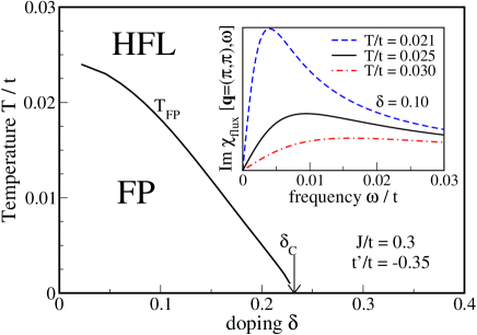
Figure 1: (Color online) Phase diagram of the $t$-$J$ model in the leading order of $1/N$ expansion where superconductivity was discarded. The instability (solid line), marked by $T_{FP}$, separates the homogeneous Fermi liquid state from the flux or $d$-CDW state and terminates at the quantum critical point at $\delta_{c}\sim 0.23$ at $T=0$. The inset shows the imaginary part of the flux susceptibility vs. $\omega$ for $\delta=0.10$ and for different temperatures [$q=(\pi,\pi)$ is the momentum where the instability occurs]. Approaching $T_{FP}$ from above the flux mode becomes better defined, accumulates weight, and softens. At $T=T_{FP}$ the flux mode reaches $\omega=0$, freezing the $d$-CDW phase. This flux mode contributes to the self-energy leading to a pseudogap and Fermi arcs features as discussed in text.

In Fig. 1, disregarding superconductivity, the solid line shows the temperature $T_{FP}$, which indicates the onset of FP instability, i.e., when the static ($i\omega_{n}=0$) flux susceptibility [Eq.(13)] diverges. At $T=0$ a phase transition occurs at the quantum critical point (QCP) placed at the critical doping $\delta_{c}$. At $T_{FP}$ a flux-mode [${\rm Im}\chi_{flux}(q=(\pi,\pi),\omega)$] reaches $\omega=0$, freezing the FP. In the inset in Fig. 1, we have plotted ${\rm Im}\chi_{flux}(q=(\pi,\pi),\omega)$ for $\delta=0.10$ for several temperatures approaching $T_{FP}/t\sim 0.018$, showing that when $T\rightarrow T_{FP}$, a low energy $d$-wave flux mode becomes soft and accumulates large spectral weight. We have used the small broadening $\eta/t=0.01$ in the analytic continuation ($i\omega_{n}\rightarrow\omega+i\eta$).

Figure 2(a) shows $\rm-Im\,\Sigma_{flux}(k,\omega)$ at $T=0$ for several dopings at the antinodal Fermi wave vector $k_{F}^{AN}$. At large doping $\delta=0.40$, $\rm-Im\Sigma_{flux}$ is weak and behaves as $\sim\omega^{2}$ at low energy. Approaching $\delta_{c}$ ($\delta=0.26$ and $\delta=0.24$), $\rm-Im\Sigma_{flux}$ increases, and the behavior at low energy is nearly linear in $\omega$ and develops structures at low energy $\omega/t\sim 0.1-0.2$. Results for the nodal Fermi vector $k_{F}^{N}$ are not shown because they are nearly negligible due to the $d$-wave character of the flux instability. Inset (i) in Fig. 2(b) shows the QP weight $Z$ at $k_{F}^{AN}$ ($Z_{flux}^{AN}$) and at $k_{F}^{N}$ ($Z_{flux}^{N}$). While $Z_{flux}^{AN}$ is strongly doping dependent and tends to zero approaching $\delta_{c}$, $Z_{flux}^{N}\sim 1$ shows that $\Sigma_{flux}$ is also strongly anisotropic on the FS.

$\Sigma_{flux}$ is written in terms of the flux or $d$-CDW susceptibility $\chi_{flux}(q,\omega)$, which shows explicitly the role played by the soft flux mode with momentum $(\pi,\pi)$ (see inset in Fig. 1). Therefore, near the antinode the QP on the FS is strongly distorted, leading to FA effects, as shown in Sec. III In addition, it is easy to check that the most important $J$ contribution to $\Sigma(k,\omega)$ enters only via $\Sigma_{flux}$.

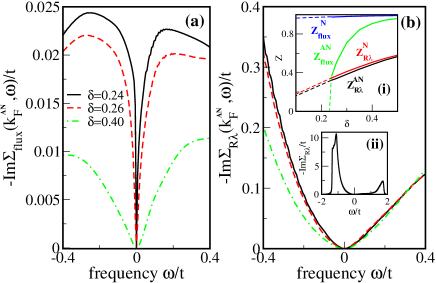
Figure 2: (Color online) The imaginary part of the two self-energy contributions, $\Sigma_{flux}$ and $\Sigma_{R\lambda}$ ($\Sigma=\Sigma_{flux}+\Sigma_{R\lambda}$). (a) Imaginary part of $\Sigma_{flux}$ at $T=0$ for several dopings approaching the QCP $\delta_{c}\sim 0.23$ for the antinodal Fermi wave vector $k_{F}^{AN}$. (b) The same as (a) for $\Sigma_{R\lambda}$. Inset (i) shows the quasiparticle weight $Z$ vs. doping for both contributions and for $k_{F}^{AN}$ and $k_{F}^{N}$. While $Z$ is weakly independent of doping and isotropic on the Fermi surface for $\Sigma_{R\lambda}$, for $\Sigma_{flux}$ $Z$ is strongly anisotropic on the FS and strongly doping dependent. Note that $Z_{flux}$ for $k_{F}^{AN}$ tends to zero approaching the QCP. In addition, at large doping, the relevant contribution is $\Sigma_{R\lambda}$. Inset (ii) shows, for $\delta=0.24$ and $k=k^{AN}_{F}$, the $\rm-Im\Sigma_{R\lambda}$ in an extended $\omega$ scale, showing that the energy scale in $\Sigma_{R\lambda}$ is large and of the order of $t$.

In $\Sigma(k,\omega)$, there is another contribution that is nearly independent of $J$. This contribution belongs to the usual charge $\delta R$ and nondouble occupancy $\delta\lambda$ channels, (the first and second components of $h_{a}$ [Eq.(7)]) and can be written asgreco08 ; foussats08

$${\mathrm{Im}}\,\Sigma_{R\lambda}(k,\omega)= - \frac{1}{N_{s}}\sum_{q}\left\{\Omega^{2}\;{\mathrm{Im}}[D_{RR}(q,\omega-\epsilon_{{k-q}})]\right.$$ (15)

$$+ \;2\;\Omega\;{\mathrm{Im}}[D_{\lambda R}(q,\omega-\epsilon_{{k-q}})]$$

$$+ \left.{\mathrm{Im}}[D_{\lambda\lambda}(q,\omega-\epsilon_{{k-q}})]\right\}$$

$$\times \left[n_{F}(-\epsilon_{{k-q}})+n_{B}(\omega-\epsilon_{{k-q}})\right],$$

where $\Omega=\frac{1}{2}(\epsilon_{{k-q}}+\omega+2\mu)$.

Figure 2(b) shows $\rm-Im\,\Sigma_{R\lambda}(k,\omega)$ at $T=0$ for $k_{F}^{AN}$ and for the same dopings as in Fig. 2(a). For $k_{F}^{N}$, $\rm Im\,\Sigma_{R\lambda}(k,\omega)$ (not shown) is nearly indistinguishable from results at $k_{F}^{AN}$, showing that $\Sigma_{R\lambda}$ is rather isotropic on the FS. In addition, $\Sigma_{R\lambda}$ behaves as $\sim\omega^{2}$ at low $\omega$, and contrary to $\Sigma_{flux}$, there is no energy scale at low energy. In inset (i) we show $Z_{R\lambda}^{AN}$ and $Z_{R\lambda}^{N}$. These results show that the doping dependence of $\Sigma_{R\lambda}$ is weaker than $\Sigma_{flux}$. Note that $Z_{R\lambda}\rightarrow 0$ when $\delta\rightarrow 0$. It is important to note that there are no structures in $\rm Im\,\Sigma_{R\lambda}(k,\omega)$ at low energy, and the main contribution appears at large energies of the order of $t$ [see inset (ii)]. Note also the strong asymmetry shown by $\Sigma_{R\lambda}$ that arises from nondouble-occupancy effects.foussats08

In summary, (a) $\Sigma_{flux}$ is strongly $J$ and doping dependent, is strongly anisotropic on the FS, and contributes at low energy, and (b) $\Sigma_{R\lambda}$ is nearly $J$ and doping independent, is strongly isotropic on the FS, and contributes at large energy. Thus, $\Sigma(k,\omega)$ can be written as the addition of two well-decoupled channels.

$${\rm Im}\,\Sigma(k,\omega)={\rm Im}\,\Sigma_{R\lambda}(k,\omega)+{\rm Im}\,\Sigma_{flux}(k,\omega)$$ (16)

Using the Kramers-Kronig relations, $\mathrm{Re}\Sigma(k,\omega)$ can be determined from $\mathrm{Im}\Sigma(k,\omega)$ and the spectral function $A(k,\omega)$, computed as usual:

$$A(k,\omega)=-\frac{1}{\pi}\frac{{\rm Im}\Sigma(k,\omega)}{[\omega-\epsilon_{k}-{\rm Re}\Sigma(k,\omega)]^{2}+{\rm Im}\Sigma(k,\omega)^{2}}$$

Before concluding this section it is important to note that at mean-field level the $d$-CDW picture leads below $T_{FP}$, where the translational symmetry is broken, to four hole pockets with low spectral weight in the outer side resembling the FAs.chakravarty03 However, as discussed in Ref. norman07, , this picture has conflicting points when compared with some ARPES data. We will show in Sec.III that the inclusion of self-energy effects in proximity to the FP instability provides a possible scenario for describing several ARPES features. Therefore, although at mean-field level the instability to the static $d$-CDW occurs below $T_{FP}$, the PG and FA formation do not require the long-range $d$-CDW state, but they do require the enhancement of fluctuations due to proximity effects. Thus, we are always located in a homogeneous state with the presence of $d$-CDW fluctuations.

III $\Sigma_{flux}$ and Fermi arcs

III.1 Topology of Fermi arcs

Since $\Sigma_{flux}$ dominates at low energy we study here the spectral functions calculated with this contribution. In Sec. IV we show that the inclusion of $\Sigma_{R\lambda}$ does not change the main conclusion obtained in this section.

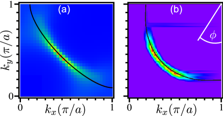
Figure 3: (Color online) (a) Intensity of the spectral function at $\omega=0$ vs $k_{x},k_{y}$ for $\delta=0.10$ and $T/t=0.025$, above but close to $T_{FP}/t\sim 0.018$. (b) The same as (a) but taken from the experimental results of Ref. norman07, for comparison. As in the experiment, (a) shows a well-defined Fermi arc whose end does not turn away from the underlying FS (solid line).

Figure 3(a) shows for $\delta=0.10$ and $T/t=0.025$ (above but close to $T_{FP}$) the spectral function intensity at zero energy vs $k_{x},k_{y}$. A well-defined FA is obtained. Similar to the experimentnorman07 [Fig. 3(b)], the end of the arc does not turn away from the underlying FS, and there is no strong suppression of the intensity at the hot spots.

In Fig. 4(a) the intensity of the spectral function on the FS is plotted as a function of the FS angle $\phi$ [defined in Fig. 3(b)] from the antinode ($\phi=0\circ$) to the node ($\phi=45\circ$). As in the experimentnorman07 [Fig. 4(b)], the intensity monotonically decreases approaching the antinode but remains finite.

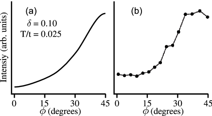
Figure 4: (Color online) (a) Intensity of the spectral function at the FS vs the Fermi surface angle $\phi$ from the antinode ($\phi=0\circ$) to the node ($\phi=45\circ$) for $\delta=0.10$ and $T/t=0.025$. (b) The same as (a) but taken from the experimental results of Ref. norman07, for comparison.

In Fig. 5(a) energy distribution curves (EDC) on the underlying FS are plotted. In agreement with the experimentnorman07 [Fig. 5(b)], near the node, there are well-defined QP peaks; approaching the antinode, the spectral functions lose intensity at $\omega=0$, become broad, and develop a PG-like feature. The presence of a PG-like feature near the antinode means that the arc plotted in Fig. 3(a) is not simply related to a decrease in the intensity from the node to the antinode but that the FS near the antinode is gapped.

Note that the present PG-like feature is not related to a true gap as in other models. It is developed dynamically in proximity to the $d$-CDW instability in the presence of strong and short-range $d$-CDW fluctuations.

In summary, the effects described in Figs. 3–5 arise from self-energy effects due to the coupling between QPs and the soft flux mode (see inset in Fig. 1) in proximity to the FP instability (solid line in Fig. 1). Since the flux mode occurs mainly with momentum $(\pi,\pi)$, the QP near the antinode is distorted, leading to FAs. Note also that since $d$-CDW fluctuations are of short-range character, in the present picture, the translational symmetry is not broken.

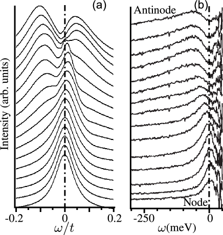
Figure 5: (a) Energy distribution curves on the underlying FS from the antinode (top) to the node (bottom) for $\delta=0.10$ and $T/t=0.025$. Near the node, well-defined QP peaks are observed. Moving from the node to the antinode, the intensity at $\omega=0$ decreases, the peak becomes broad, and a pseudogap feature is developed. (b) The same as (a) but taken from the experimental results of Ref. norman07, for comparison.

III.2 Temperature dependence of the Fermi arcs

The temperature dependence of the length of the FAs is puzzling. In spite of different views and interpretations most reports agree on the fact that the observed FAs depend on temperature. While there are reports that claim that the length of FAs collapse to one isolated pointkanigel06 ; kanigel07 (nodal metal) at $T=0$, others suggest a less-strong temperature dependence.jonson3 ; storey08 In models discussed in Ref. norman07, the temperature dependence of the length of the arcs arises after assuming a temperature dependence for $\Delta_{k}$ or for the lifetime broadening $\Gamma$. In this subsection it is shown that the temperature dependence of the FAs emerges, in the framework of the present approach, without adjustable parameters, showing that the temperature dependence of the length of the arcs is entangled to their origin.

Figure 6 shows the plot, for $\delta=0.10$, of FA for different temperatures. Clearly, the length of the arcs decreases when temperature decreases. We note that the temperature dependence of the arcs seems to be weaker than in some experimentskanigel06 but closer to othersjonson3 ; storey08 (this point is further discussed in Sec. IV). Beyond a quantitative comparison, the because no phenomenological parameter is assumed to be temperature dependent in the present model, the results can be considered satisfactory. Figure 7 plots the spectral function intensity on the FS for several temperatures normalized to the intensity at $k_{F}^{N}$. Consistent with the picture in Fig. 6, with decreasing temperature, the intensity is more concentrated around the node.

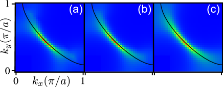
Figure 6: (Color online) Fermi arc for $\delta=0.10$ for several temperatures: (a) $T/t=0.021$, (b) $T/t=0.025$, and (c) $T/t=0.050$. Similar to experiments, when the temperature increases, the length of the arc increases.

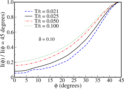
Figure 7: (Color online) (a) Intensity of the spectral function (normalized to the intensity at the node ) at the FS vs. $\phi$ for $\delta=0.10$ and for several temperatures. When the temperature decreases toward $T_{FP}$, the intensity is more and more concentrated around the node.

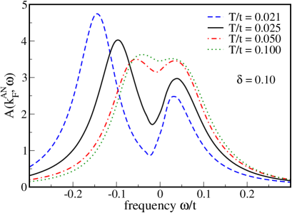
Figure 8: (Color online) EDC at $k_{F}^{AN}$ for $\delta=0.10$ and for the same temperatures as in Fig. 7. As in experiments when temperature increases, the PG feature fades out. Although the leading edge of the pseudogap partially closes, a filling is also observed, as in the experiments.

Finally, Fig. 8 shows EDC at $k_{F}^{AN}$ for the same temperatures as in Fig. 7. Although the PG feature partially closeshashimoto10 with increasing temperature, a filling is also observed.norman98 ; kanigel06 ; kanigel07 This feature is in agreement with experiments and in contrast to results from mean-field calculations where only a closure is expected.

It is worth mentioning that while the arcs discussed here are dynamically generated, they necessarily occur at finite temperature. The present approach should be distinguished from other oneskampf ; lorenzana ; choi where a phenomenological fitted susceptibility without explicit temperature dependence is proposed.

III.3 Doping dependence of the Fermi arcs

It is well known that with increasing doping, the PG feature closeskim98 ; kaminski05 and, simultaneously, the length of the arcs increases.kanigel07 For describing this behavior, models discussed in Ref. norman07, need to assume a phenomenological doping dependence for the PG. In this subsection we will show that arcs whose length increases with increasing doping can be naturally discussed in the present context.

In Fig. 9 the FA is shown for several dopings and for a fixed temperature $T/t=0.025$. With increasing doping, the length of the arcs increases, in agreement with experiments. Figure 10 shows EDC at $k_{F}^{AN}$ for several dopings. When doping increases, the PG-like feature closes and, simultaneously, the intensity increases at $\omega=0$.

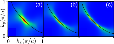
Figure 9: (Color online) Fermi arc for $T/t=0.025$ and for several dopings: (a) $\delta=0.05$, (b) $\delta=0.10$, and (c) $\delta=0.15$. As in experiments when doping increases toward overdoped, the length of the arc increases.

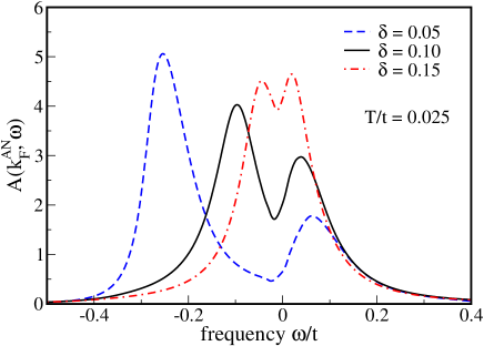
Figure 10: (Color online) EDC at $k_{F}^{AN}$ for $T/t=0.025$ and for the same dopings as in Fig. 9. Like in experiments when doping increases, the PG feature washes out in a way consistent with the increment of the length of the arc reported in Fig. 9.

In summary, in Secs. III B and III C it is shown that with increasing doping and temperature the PG-like feature and the FA fade out like in the experiments. The origin for this behavior is easy to understand: By increasing doping and temperature we leave out the instability line $T_{FP}$. Then, the flux mode is less efficient, self-energy effects become weaker, and the long FS is smoothly recovered. It is important to note that from our approach $T^{*}$ must be distinguished from a true phase transition. Here at $T^{*}>T_{FP}$, where the PG features vanish, there is not a phase transition but a smooth crossover.tallon01 Finally, note that if $t=0.4eV$, the energy scale for the pseudogap and temperature is of the order of the experiment.

III.4 Main characteristics of $\Sigma_{flux}$

For a complete discussion about the origin of the arcs we have investigated the main characteristics of $\Sigma_{flux}$. Figure 11 shows $\rm-Im\Sigma_{flux}$ at $k_{F}^{N}$ and $k_{F}^{AN}$ for $T/t=0.025$ and $\delta=0.10$ [Fig. 11(a)], $\delta=0.25$ [Fig. 11(b)], and $\delta=0.40$ [Fig. 11(c)]. At $k_{F}^{N}$, $\rm-Im\Sigma_{flux}$ is smaller than for $k_{F}^{AN}$, leading to a well-defined and nearly no renormalized QP peak in the nodal direction [Fig. 5(a)]. However, the behavior at $k_{F}^{AN}$ is very different, especially at low doping. Instead of a minimum at $\omega=0$, $\rm-Im\Sigma_{flux}$ shows a maximum clearly observed for $\delta=0.10$ [Fig. 11(a)]. This behavior, which is in contrast to the expected results from the usual many-body physics,katanin03 ; dellanna06 is the main reason for the PG and FA formation. With increasing doping, the maximum at $\omega\sim 0$ washes out, and for large doping, $\rm-Im\Sigma_{flux}$ develops the expected minimum at $\omega=0$. [See results for $\delta=0.40$ in Fig. 11(c)].

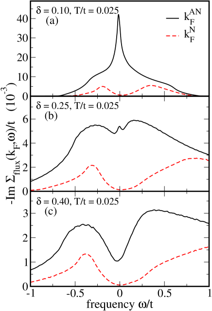
Figure 11: (Color online) $\rm-Im\Sigma_{flux}$ for $T/t=0.025$ at $k_{F}^{AN}$ and $k_{F}^{N}$ for (a) $\delta=0.10$, (b) $\delta=0.25$, and (c) $\delta=0.40$. For all dopings, $\rm-Im\Sigma_{flux}$ at $k_{F}^{N}$ (dashed line) is smaller than the corresponding results at $k_{F}^{AN}$ and shows the expected minimum at $\omega=0$. However, the behavior at $k_{F}^{AN}$ is very different. With decreasing doping, $\rm-Im\Sigma_{flux}$ (solid line) increases, and a maximum, instead of a minimum, is developed at $\omega\sim 0$. This behavior, which occurs only at finite temperature, is the cause for the dynamical generation of the arcs and the PG feature. For large doping (see results for $\delta=0.40$), $\rm-Im\Sigma_{flux}$ is small and depicts the expected behavior from the usual many-body theory, i.e., it has a minimum at $\omega=0$. This behavior is consistent with the fact that no arcs and no PG features are obtained for large doping.

IV Inclusion of $\Sigma_{R\lambda}$

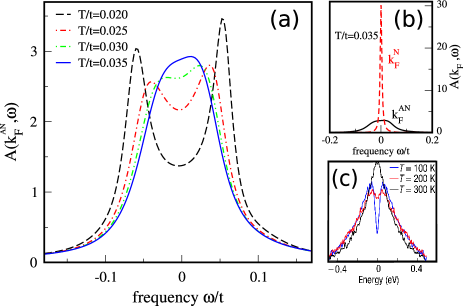
Figure 12: (Color online) (a) EDC at $k_{F}^{AN}$ for $\delta=0.10$ and for several temperatures calculated using both contributions, $\Sigma_{R\lambda}$ and $\Sigma_{flux}$. Note that the inclusion of $\Sigma_{R\lambda}$ does not change the main conclusion obtained when only $\Sigma_{flux}$ is considered. As in the experiments, when temperature increases, the PG feature washes out. As in Fig. 8, although the leading edge of the pseudogap closes, a filling is also observed. Note that different from the calculation with only $\Sigma_{flux}$ (Fig. 8), at $T/t=0.035$ a full peak is recovered. (b) Spectral functions at $k_{F}^{AN}$ and $k_{F}^{N}$ for $T/t=0.035$. (c) Experimental results taken from Ref. kanigel06, for comparison.

It was shown (Fig. 2) that the energy scale in $\Sigma_{R\lambda}$ is much larger ($\sim t$) than the energy scale in $\Sigma_{flux}$. Although this fact implies (as shown in Sec. III) that $\Sigma_{flux}$ is the relevant contribution for triggering the low-energy PG features, in this section, for completeness, we discuss the role of $\Sigma_{R\lambda}$ in the spectral functions. It was discussed in Sec. IIIB that the PG closes and fills smoothly with increasing temperature (see Fig. 8). In this section we show that the only role of including $\Sigma_{R\lambda}$ is to improve the vanishing of the PG.add

Figure 12(a) shows EDC for $\delta=0.10$ for several temperatures at $k_{F}^{AN}$. This figure shows that with increasing temperature the PG fills and a peak at $\omega=0$ emerges at $T/t\sim 0.035$. Note that in Fig. 8, where only $\Sigma_{flux}$ was considered, even at the high temperature $T/t=0.1$ the maximum of $A(k,\omega)$ is not yet fully formed at $\omega=0$. In Fig. 12(c) we have reproduced, for comparison, the experimental results,kanigel06 showing qualitative agreement between theory and experiment. In Fig. 12(b) we plot, for $T/t=0.035$, $A(k,\omega)$ for $k_{F}^{AN}$ (solid line) and $k_{F}^{N}$ (dashed line). Althought the entire FS is ungapped at this temperature, the QP are better defined near the node, as in the experiment.kim98

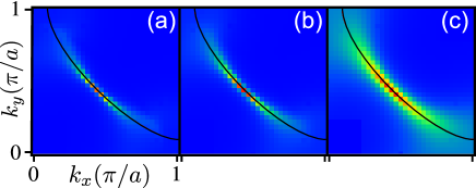
Figure 13: (Color online) Fermi arc for the same temperatures as in Fig. 6, (a) $T/t=0.021$, (b) $T/t=0.025$, and (c) $T/t=0.050$, but calculated using both $\Sigma_{R\lambda}$ and $\Sigma_{flux}$. As in Fig. 6, when temperature increases the length of the arc increases.

Figure 13 shows the spectral function intensity at $\omega=0$ vs $k_{x}$,$k_{y}$ for $\delta=0.10$ and for the same temperatures as in Fig. 6. At low temperatures a FA is obtained, and its length increases with increasing $T$. Note that while the FS is expected to be gapped near the antinode for $T/t=0.025$ (dot-dashed line in Fig. 12), for $T/t=0.050$ the full FS is ungapped.

In summary, $\Sigma_{R\lambda}$ does not modify the main conclusion obtained in Sec. III. We have shown that its inclusion enhances the pseudogap closing and filling, and contributes to a faster reconstruction of the entire FS with increasing temperature.

V Discussion and conclusion

The large-$N$ approach in the $t$-$J$ model leads, beyond the mean-field level, to two distinct dynamical self-energy contributions, namely, $\Sigma_{R\lambda}$ and $\Sigma_{flux}$. In this paper we have analyzed the role of these contributions in ARPES.

The main characteristics of $\Sigma_{flux}$ are the following. $\Sigma_{flux}$ is strongly anisotropic on the FS, strongly doping dependent, and dominated by $J$ (if $J=0$ $\Sigma_{flux}$ is negligible), and it contributes at low energy. Thus, $\Sigma_{flux}$ is the relevant contribution for describing the Fermi arcs and pseudogap features.

The fact that $\Sigma_{flux}$ is mainly dominated by $J$ may be understood as follows. At mean-field level the $t$-$J$ model shows (and only for finite $J$) the flux or $d$-CDW phase below a temperature $T_{FP}$. $T_{FP}$ decreases with increasing doping, approaching the QCP at $\delta_{c}$ and $T=0$. In the proximity of $T_{FP}$, $d$-CDW fluctuations enter $\Sigma_{flux}$ [Eq.(12)]. Since $d$-CDW fluctuations favor scattering between electrons with momentum transfer $q\sim(\pi,\pi)$, the FS near the antinode is gaped, leading to Fermi arcs being dynamically generated. With increasing doping and temperature beyond $\delta_{c}$ and $T_{FP}$, respectively, $d$-CDW fluctuations become weak, and the Fermi arcs and the pseudogap wash out, in agreement with experiments.

It is important to note that the present picture does not require any phenomenological parametrization for the pseudogap or the lifetime broadening and their temperature and doping dependence. It is only necessary to be in the proximity of the $d$-CDW instability or in a situation with strong short-range fluctuations. In other words, under the present approach Fermi arcs originate dynamically due to the interaction between carriers and short-range and short-living $d$-CDW fluctuations, implying that long-range order is not broken.

The present picture has similarities with some phenomenological approacheschoi where the pseudogap and Fermi arcs are described in a scenario where fermions interact with bosonic fluctuations of some special order. Importantly, our description offers a microscopic derivation from the $t$-$J$ model, and, as a corollary, the fluctuating spectrum is obtained with no assumptions of any fitted phenomenological parameter, such as coupling, correlation length, or bosonic frequency. Note that near the flux instability the flux mode (inset in Fig. 1) is overdamped and intrinsically temperature dependent and can not be easily considered as an Einstein mode as in other approaches.kampf ; lorenzana ; choi

A recent ARPES experimenthashimoto10 suggests a similar scenario to that presented here, i.e., density wave fluctuations without long-range order. As in that experiment, in our theory, the existence (and persistence with decreasing temperature) of broad and gapped spectral features near the antinode means that we are not sitting in a phase with long-range order. It is worth mentioning that under the present approach, below the mean-field temperature $T_{FP}$ the long-range $d$-CDW order occurs; that is, a true gap is formed, and sharp spectral features are expected with the corresponding reconstruction of the FS in the form of pockets.greco09 From an experimental point of view the existence of long-range order in underdoped cuprates is controversial and is tied to the following facts. (a) Some ARPES experiments show well-defined spectral peaks near the antinode in the superconducting state, while others show broad structures (see Ref. vishik, and references therein). (b) While some experiments support the existence of a second order parameter, distinct from but coexisting (and competing) with superconductivity,terashima07 ; hashimoto10 ; yoshida09 ; kondo07 ; kondo09 ; lee07 ; tanaka06 ; ma08 others claim to observe only one gap feature.norman98 ; kanigel06 ; kanigel07 ; shi (c) While quantum oscillationsQOs and some ARPES experiments show a reconstruction of the FS in the form of pockets,Nd ; meng ; jonson1 ; jonson2 ; jonson3 other reports show only arcs.kanigel06 ; kanigel07 ; norman07 Although it is not our aim to solve these puzzles (which requires more theoretical and experimental work), we have shown that several aspects related to the Fermi arc phenomenology can be explained by $d$-CDW proximity effects, showing that this picture is not necessarily inconsistent with the notion of arcs.

The characteristics of $\Sigma_{R\lambda}$ are very different from those of $\Sigma_{flux}$. $\Sigma_{R\lambda}$ is dominated by the usual charge channel and (nearly) independent of $J$. Thus, this is the relevant contribution for the $J=0$ case. In addition, it is strongly asymmetric in $\omega$ around the FS due to nondouble-occupancy effects, rather isotropic on the FS, and rather constant as a function of doping (for low to intermediate doping).foussats08 Finally, it contributes at large energy of the order of $t$. Although $\Sigma_{R\lambda}$ is not responsible for the pseudogap and Fermi arc formation, it gives an additional contribution to the temperature vanishing of the pseudogap.

$\Sigma_{R\lambda}$ and $\Sigma_{flux}$ may also play a role in describing other experiments in cuprates. (a) Since $\Sigma_{R\lambda}$ shows high- energy contributions, it leads, in the spectral functions, to incoherent structures at high binding energy, which offers a possible explanationfoussats08 ; greco07 for the high-energy features or waterfall effects observed in cuprates.xie07 ; meevasana07 ; graf07 ; zhang08 Other theoreticalchinos ; zemljic and experimentalzhang08 reports show a similar conclusion. (b) The existence of two self-energy contributions is also consistent with recent angle-dependent magnetoresistance (ADMR) experiments.abdel06 ; abdel07 ; french09 These experiments show two different inelastic scattering rates with similar characteristics to the self-energy behavior discussed here, i.e., a strongly-doping-dependent and anisotropic scattering rate on the FS and another one that is weakly doping dependent and isotropic on the FS. Recently, ADMR experiments were discussed in the context of the present approach.buzon10

Here we want to comment on the recent progress on DCA. As discussed in Sec. I DCA shows the presence of a pseudogaphuscroft01 ; macridin06 and Fermi arcs.parcollet04 ; werner09 ; lin10 We wish to mention here the similarities between our results and those in DCA. For instance, the pole feature at $\omega\sim 0$ and near the antinode that occurs in $Im\Sigma$ (Fig. 11), which diminishes with increasing temperature and doping, is in remarkable agreement with similar results discussed in Ref. lin10, . This behavior for the self-energy leads also to a similar doping and temperature dependence for the PG and FAs. Note that in Ref. lin10, the temperature filling of the PG as discussed in the present paperwas also obtained. We note again that our results do not require the static long-range order of the $d$-CDW. What is needed is the enhancement of the $d$-CDW susceptibility due to fluctuations, as can be seen in the inset of Fig. 1. Interestingly, although the static $d$-CDW state was not found in Ref. macridin04, , an enhancement of the $d$-CDW susceptibility was obtained. Finally, it is worth mentioning that although the origin of the PG and FAs is presumably of antiferromagnetic nature,huscroft01 ; macridin06 a recent reportlin10 is not conclusive about this affirmation. It is the aim of the present paper to show that $d$-CDW fluctuations may contribute to the PG and FAs formation.

Although of one could certainly suppose that the large-$N$ is a particular approximation and some results may depend on its details, we think that our theory contains features that can be expected, qualitatively, in cuprates and in the $t$-$J$ model. Since the low-energy pseudogap feature increases with decreasing doping, it is reasonable to think that the pseudogap is associated with the same energy scale as the antiferromagnetism, i.e., $J$. This fact is contained in $\Sigma_{flux}$. On the other hand, there is a larger energy scale, the hopping $t$, which, together with nondouble-occupancy effects, enters through $\Sigma_{R\lambda}$.

Finally, it is worth mentioning that besides $d$-CDW, other instabilities like stripes,stripes antiferromagnetism,AF and Pomeranchukpomeranchuk have been proposed to exist at low doping in cuprates. Thus, it is important to perform similar calculations for those cases and compare different predictions.

Acknowledgments

The authors thank H. Parent for suggestions on the presentation of the paper. A.G. thanks R.-H. He, W. Metzner, A. Muramatsu, Y. Yamase, and R. Zeyher for valuable discussions and the Max Planck Institute (Stuttgart) and the University of Stuttgart for hospitality.

References

- (1) T. Timusk and B. Statt, Rep. Prog. Phys. 62, 61 (1999).
- (2) S. Hüfner, M.A. Hossain, A. Damascelli, and G.A. Sawastzky, Rep. Prog. Phys. 71, 062501 (2008).
- (3) M. R. Norman, D. Pines and C. Kallin, Adv. Phys. 54, 715 (2005).
- (4) A. Damascelli, Z. Hussain, and Z.-X.Shen, Rev. Mod. Phys. 75, 473 (2003).
- (5) M.R. Norman et al., Nature (London) 392, 157 (1998).
- (6) A. Kanigel et al., Nature Physics 2, 447 (2006).
- (7) A. Kanigel et al., Phys. Rev. Lett. 99, 157001 (2007).
- (8) M. Shi et al., Phys. Rev. Lett. 101, 047002 (2008).
- (9) K. Terashima et al., Phys. Rev. Lett. 99, 017003 (2007).
- (10) M. Hashimoto et al., Nature Phys. 4, 414 (2010).
- (11) T. Yoshida et al., Phys. Rev. Lett. 103, 037004 (2009).
- (12) T. Kondo et al., Phys. Rev. Lett. 98, 267004 (2007).
- (13) T. Kondo et al., Nature 457, 296 (2009).
- (14) K. Tanaka, et al., Science 314, 910 (2006).
- (15) W.S. Lee, et al., Nature 450, 81 (2007).
- (16) J.-H. Ma et al., Phys. Rev. Lett. 101, 207002 (2008).
- (17) J. Chang et al., New. J. Phy. 10, 103016 (2008).
- (18) J. Meng et al., Nature 462, 335 (2009).
- (19) H.-B. Yang et al., Nature 456, 77 (2008).
- (20) K.-Y. Yang et al., Euro Phys. Lett. 86, 37002 (2009).
- (21) H.-B. Yang et al., arXiv: 1008.3121.
- (22) A. Sherman and M. Schreiber, Phys. Rev. B 55, R712 (1997).
- (23) C. Huscroft et al., Phys. Rev. Lett. 86, 139 (2001).
- (24) A. Macridin et al., Phys. Rev. Lett. 97, 036401 (2004).
- (25) O. Parcollet, G. Biroli, and G. Kotliar, Phys. Rev. Lett. 92, 226402 (2004).
- (26) P. Werner et al., Phys. Rev. B 80, 045120 (2009).
- (27) N. Lin, E. Gull, and A. Millis, Phys. Rev. B 82, 045104 (2010).
- (28) M.R. Norman et al., Phys. Rev. B 76, 174501 (2007).
- (29) S. Chakravarty, R. B. Laughlin, D. K. Morr, and C. Nayak, Phys. Rev. B 63, 094503 (2001).
- (30) K.-Y. Yang, T. M. Rice, and F.-C Zhang, Phys. Rev. B 73, 174501 (2006).
- (31) M.R. Norman, M. Randeria, H. Ding, and J.C. Campuzano, Phys. Rev. B 57, R11093 (1998).
- (32) P. W. Anderson, Science 235, 1196 (1987).
- (33) F. C. Zhang and T. M. Rice, Phys. Rev. B 37, 3759 (1988).
- (34) K. A. Chao, J. Spałek, and A. M. Oleś, J. Phys. C 10, L271 (1977); Phys. Rev. B 18, 3453 (1978).
- (35) Z. Wang, Int. Mod. Phys. B 6, 603 (1992).
- (36) R. Zeyher and M. L. Kulić, Phys.Rev. B 54, 8985(1996).
- (37) A. Foussats and A. Greco, Phys. Rev. B 70, 205123 (2004).
- (38) I. Affleck and J.B. Marston, Phys. Rev. B 37, 3774 (1988).
- (39) G. Kotliar, Phys. Rev. B 37, 3664 (1988).
- (40) D.C. Morse and T.C. Lubensky, Phys. Rev. B 43, 10436 (1991).
- (41) E. Cappelluti and R. Zeyher, Phys. Rev. B 59, 6475 (1999).
- (42) P. W. Leung, Phys. Rev. B 62, R6112 (2000).
- (43) A. Macridin, M.Jarrel, and Th. Maier, Phys. Rev. B 70, 113105 (2004).
- (44) A. Sherman and M. Schreiber, Phys. Rev. B 77, 155117 (2008).
- (45) A. Greco, Phys. Rev. B 77, 092503 (2008).
- (46) A. Greco, Phys. Rev. Lett. 103, 217001 (2009).
- (47) M. Bejas, A. Greco, and Foussats, Phys. Rev. B 73, 245104 (2006).
- (48) A. Foussats, A. Greco, and M. Bejas, Phys. Rev. B 78, 153110 (2008).
- (49) S. Chakravary, C. Nayak, and S. Tewari, Phys. Rev. B 68, 100504 (2003).
- (50) J. G. Storey, J. L. Tallon, and G. V. M. Williams, Phys. Rev. B 78, 140506 (2008).
- (51) A. P. Kampf and J. R. Schrieffer, Phys. Rev. B 42, 7967 (1990).
- (52) M. Grilli, G. Seibold, A. Di Ciolo, and J. Lorenzana, Phys. Rev. B 79, 125111 (2009).
- (53) H.-Y. Choi and S. H. Hong, Phys. Rev. B 82, 094509 (2010).
- (54) C. Kim et al., Phys. Rev. Lett. 80, 4245 (1998).
- (55) A. Kamiski et al., Phys. Rev. B 71, 014517 (2005).
- (56) J.L. Tallon and J.W. Loran, Physica C 349, 53 (2001).
- (57) A. A. Katanin and A. P. Kampf, Phys. Rev. Lett. 93, 106406 (2004).
- (58) L. Dell’Anna and W. Metzner, Phys. Rev. B 73, 045127 (2006).
- (59) After a comparison with the experiments, we have found that a reduction of the contribution of by a factor of four is appropiated. A possible reason may stem from the fact that the large- approach overstimates charge fluctuations over other fluctuations such as spin excitations (see Ref.[foussats04, ] for discussions).
- (60) I. M. Vishik et al., New. J. Phys. 12, 105008 (2010).
- (61) S. E. Sebastian et al., Nature 454, 200 (2008).
- (62) A. Greco, Solid State Comm. 142, 318 (2007).
- (63) B. P. Xie et al., Phys. Rev. Lett. 98, 147001 (2007).
- (64) W. Meevasana et al., Phys. Rev. B 75, 174506 (2007).
- (65) J. Graf et al., Phys. Rev. Lett. 98, 067004 (2007).
- (66) W. Zhang et al., Phys. Rev. Lett. 101, 017002 (2008).
- (67) Fei Tan and Qiang-Hua Wang, Phys. Rev. Lett. 100, 117004 (2008).
- (68) M. M. Zemljic̆, P. Prelovšek and T. Tohyama, Phys. Rev. Lett. 100, 036402 (2008).
- (69) M. Abdel-Jawad et al., Nature Phys. 2, 821 (2006).
- (70) M. Abdel-Jawad et al., Phys. Rev. Lett. 99, 107002 (2007).
- (71) M.M. J. French et al, New J. Phys. 11, 055057 (2009).
- (72) G. Buzon and A. Greco, Phys. Rev. B 82, 054526 (2010).
- (73) M. Vojta and S. Sachdev, Phys. Rev. Lett. 83, 3916 (1999).
- (74) H. Yamase and H. Kohno, Phys. Rev. B 69, 104526 (2004).
- (75) H. Yamase and H. Kohno, J. Phys. Soc. Jpn. 69, 2151 (2000). Ch. Halboth and W. Metzner, Phys. Rev. Lett. 85, 5162 (2000).