Is the metallicity of their hosts a good measure of the metallicity of Type Ia supernovae?

Abstract

The efficient use of Type Ia supernovae (SNIa) for cosmological studies requires knowledge of any parameter that can affect their luminosity in either systematic or statistical ways. Observational samples of SNIa commonly use the metallicity of the host galaxy, $Z_{\mathrm{host}}$, as an estimator of the supernova progenitor metallicity, $Z_{\mathrm{Ia}}$, that is one of the primary factors affecting SNIa magnitude. Here, we present a theoretical study of the relationship between $Z_{\mathrm{Ia}}$ and $Z_{\mathrm{host}}$. We follow the chemical evolution of homogeneous galaxy models together with the evolution of the supernova rates in order to evaluate the metallicity distribution function, $\mathrm{MDF}(\Delta Z)$, i.e. the probability that the logarithm of the metallicity of a SNIa exploding now differs in less than $\Delta Z$ from that of its host. We analyse several model galaxies aimed to represent from active to passive galaxies, including dwarf galaxies prone to experience supernova driven outflows. We analyse as well the sensitivity of the MDF to the most uncertain ingredients of our approach: IMF, star-formation law, stellar lifetime, stellar yields, and SNIa delay-time distribution (DTD). Our results show a remarkable degree of agreement between the mean $\bar{Z}_{\mathrm{Ia}}$ in a galaxy and its $Z_{\mathrm{host}}$ when they both are measured as the CNO abundance, especially if the DTD peaks at small time delays, while the average Fe abundance of host and SNIa may differ up to 0.4-0.6 dex in passive galaxies. The dispersion of $Z_{\mathrm{Ia}}$ in active galaxy models is quite small, meaning that $Z_{\mathrm{host}}$ is a quite good estimator of the supernova metallicity. Passive galaxies present a larger dispersion, which is more pronounced in low mass galaxies. We present a procedure to generate random SNIa metallicities, given the host metallicity. We also discuss the use of different metallicity indicators: Fe vs. O, and gas-phase metallicity vs. stellar metallicity. Finally, the results of the application of our formalism to a galactic catalogue (VESPA) suggest that SNIa come, in average, from small metallicity progenitors both at low redshifts (contrary to expectations) and in galaxies with high star-formation activity. In spite of large uncertainties in the metallicities derived from the catalogue, the gross trends of $\bar{Z}_{\mathrm{Ia}}$ vs. $Z_{\mathrm{host}}$ obtained from VESPA for different galaxy types are roughly consistent with our theoretical estimates.

1 Introduction

Metallicity is one of the few progenitor attributes that can affect the luminosity of Type Ia supernovae (SNIa), with important consequences for their use as cosmological standard candles (Domínguez et al., 2001; Timmes et al., 2003; Kasen et al., 2009). Recently, Bravo et al. (2010) analysed the metallicity as a source of dispersion in the light-curve width-luminosity relationship and found that deriving supernova luminosities from light curve shapes without accounting for the supernova metallicity might lead to systematic errors of up to 0.5 mag. From an observational point of view, the dependence of SNIa luminosities on metallicity might originate a systematic error of $\sim 9$% in the measurement of the dark energy equation of state $w$ (Gallagher et al., 2008; Sullivan et al., 2010), comparable to the current statistical uncertainties. Sullivan et al. (2010) proposed to include the host properties (galaxy mass and metallicity) into the SNIa light-curve fitters in order to correct for these systematic errors.

Up to now, attempts to measure the metallicity directly from supernova observations have been scarce and their results uncertain (Lentz et al., 2000; Taubenberger et al., 2008). Measuring the metallicity, $Z$, from the X-ray emission of supernova remnants is a promising alternative but as yet has been only applied to a single supernova (Badenes et al., 2008), although there are prospects to extend this analysis to further remnants (Badenes, 2010; Yamaguchi & Koyama, 2010). An alternative venue is to estimate the supernova metallicity as the mean $Z$ of its environment (Badenes et al., 2009) - this can be done for statistically significant samples of SNe in nearby galaxies by taking advantage of the long evolutionary timescales of their supernova remnants (Badenes et al., 2010).

Excluding these studies based on individual objects or supernova remnants, the vast majority of our knowledge about the metallicity of Type Ia SN progenitors has been assembled by measuring the bulk properties of their entire host galaxies. Hamuy et al. (2000) looked for galactic age or metal content correlations with SNIa luminosity in star-forming hosts, but their results were ambiguous. Gallagher et al. (2005) studied the correlations between SNIa properties and galaxy metallicity or, more precisely, its oxygen abundance as determined from emission lines in the integrated spectra of star-forming hosts. Ellis et al. (2008) looked for systematic trends of SNIa UV spectra with metallicity of the host galaxy, and found that the spectral variations were much larger than predicted by theoretical models. Prieto et al. (2008) studied the metallicity of all the star-forming galaxies in the Sloan Digital Sky Survey (SDSS) catalogue with redshifts in the range $0.01<z<0.04$ that hosted SNe of some kind and noted that SNIa occur in a wide range of metallicities, as low as 0.25 solar. Cooper et al. (2009), using data from the SDSS and Supernova Survey concluded that prompt SNIa are more luminous in metal-poor systems. Gallagher et al. (2008) and Howell et al. (2009), using different methodologies to estimate the metallicity of SNIa hosts, arrived to opposite conclusions with respect to the dependence of supernova luminosity on $Z$, although these discrepancies might have been solved recently (Kelly et al., 2010). We note that most of the previous work has focused on comparisons between the empirical observationally-determined relationship between the metallicity of hosts and their SNIa luminosities on the one hand (e.g. Howell et al., 2009) and theoretical predictions of correlations between the supernova metallicity and luminosity on the other hand (e.g. Timmes et al., 2003), thus assuming implicitly that both metallicities are somehow tied.

Estimating the metallicity of an entire galaxy is a complex task, involving many different observational and theoretical challenges. On the observational side, different tracers exist for both gas-phase and stellar metallicities, each with their own advantages and disadvantages (Binney & Merrifield, 1998). On the theoretical side, complex modelling of the observations is often required to arrive at a numerical estimate of the metallicity, which introduces biases and uncertainties that depend on the specific technique used (e.g. Conroy et al., 2009). Gallagher et al. (2008) measured the host metallicity from absorption lines of Fe at two wavelengths, thus testing the gas-phase in early-type galaxies, using single-age single-metallicity stellar population models. Then, to derive metallicity, they assumed solar elemental ratios in the galactic interstellar medium (ISM). Howell et al. (2009) determined the host metallicity indirectly. In a first step, they determined the host mass from spectral energy distribution fits to galaxy photometry. Next, they applied the well-known mass-metallicity relationship (Tremonti et al., 2004), also valid for the gas-phase. The Tremonti et al. (2004) mass-metallicity relationship was determined in turn through measures of the nebular emission lines of oxygen in star-forming galaxies. Cid Fernandes et al. (2005) compared the stellar metallicities to those of the gas-phase (measured through the oxygen abundance) for several thousand galaxies in the SDSS. They found that the relationship between both metallicities is non-linear, with a shallower than linear dependence of the gas-phase oxygen abundance on the stellar metallicity, and a large scatter of data points.

The question we want to address in this work is: What is the relationship between the metallicity of a SNIa and that of its host galaxy? Given the complexity of the problem we want to address it from a statistical point of view, aiming to determine a distribution function for the difference of metallicities between the supernova and its host. Our approach is based on calculations of galactic chemical evolution together with the evolution of the supernova rate. In order to understand which the best estimators of SNIa metallicity are we study the correlations between SNIa metallicity and different observational tracers of host metallicity: Fe vs. O in the gas-phase and stellar vs. gas-phase metallicity. In order to keep simplicity, we use homogeneous one-zone galactic chemical evolution models, disregarding spatial variations within each galaxy. Taking into account the spatial variations of metallicity would increase the scatter and corrections modelled in this paper.

The plan of the paper is as follows. In Section 2, we describe the theoretical framework we adopt in order to derive the statistical properties of the metallicities of SNIa compared to that of their host galaxies. In the next section, we analyse the results, with particular emphasis on the reliability of different host metallicity measures as estimators of SNIa metallicity. Among the tracers that we consider, we rank highest the measure of SNIa metallicity through the gas-phase metallicity of its host. We pay special attention to the influence of the assumed Delay Time Distribution (DTD) of SNIa. It turns out that the metallicity of an average SNIa is closer to that of its host if the DTD peaks at small time delays, as the DTD of Maoz et al. (2010b), than if the SNIa rate follows the rate of formation of white dwarfs, as proposed by Pritchet et al. (2008). In Section 4 we explore the possibility of using current galactic catalogues, such as SDSS and VESPA, to derive the metallicity distribution function of SNIa. Finally, in Section 5 we draw our conclusions.

2 The chemical evolution of galaxies and their SNIa

2.1 SNIa Metallicity Distribution Function

We define the metallicity probability density of SNIa, $P^{\prime}(\Delta Z)$ as the probability that a SNIa comes from a progenitor whose metallicity logarithm differs from the logarithm of its host metallicity, $Z_{\mathrm{host}}$, in:

$$\Delta Z\equiv\log\left(Z_{\mathrm{Ia}}/Z_{\mathrm{host}}\right)\,.$$ (1)

Similarly, we define the metallicity distribution function (MDF) of SNIa as the cumulative metallicity probability, i.e. the probability that the difference between the logarithm of the metallicity of the SNIa progenitor and that of the host is smaller than $\Delta Z$ (note that this means $\Delta Z$ larger in absolute value in the usual case that the SNIa metallicity is smaller than the host’s one),

$$\mathrm{MDF}\left(\Delta Z\right)=\int_{-\infty}^{\Delta Z}P^{\prime}\left(\Delta Z\right)\mathrm{d}\Delta Z\,.$$ (2)

We give additional details about the procedure we use to compute $P^{\prime}\left(\Delta Z\right)$ at the end of Section 2.3. We further define the “metallicity correction”, $\Delta\bar{Z}$, as the mean value of $\Delta Z$, i.e.:

$$\Delta\bar{Z}\equiv\overline{\log}\left(Z_{\mathrm{Ia}}/Z_{\mathrm{host}}\right)\,.$$ (3)

The present rate of SNIa explosions in a given host, $R_{\mathrm{Ia}}(t)$, is the convolution over time of the Star Formation Rate (SFR), $S$, and the DTD, $\Psi$:

$$R_{\mathrm{Ia}}=\int_{0}^{t}S(t^{\prime})\Psi(t-t^{\prime})dt^{\prime}\,.$$ (4)

The probability that a SNIa that explodes now (at time $t$) comes from a progenitor born at time $t^{\prime}=t-\tau$ is:

$$P_{\mathrm{Ia}}\left(\tau\right)=S(t-\tau)\Psi(\tau)/R_{\mathrm{Ia}}(t)\,,$$ (5)

where $\tau$ is the time spanned since progenitor birth to the moment the host is being observed, which we will call look-back time, and $t$ is the cosmic time. Finally, the knowledge of $P_{\mathrm{Ia}}$ vs. time and the metallicity evolution, $Z(t)$, allows to construct the MDF of SNIa.

We have used two different prescriptions for the DTD: those of Pritchet et al. (2008) and Maoz et al. (2010b, in the following M10b). As we will show later in Section 3.3, the DTD is the most influential ingredient for the determination of the MDF of SNIa.

Pritchet et al. (2008, in the following P08) found that the observational rate of SNIa is a constant fraction, $\sim 1\%$ of the stellar death rate and independent of the SFR. Later, Raskin et al. (2009) used a different method to confirm the results of P08, i.e. the rate of SNIa traces the rate of formation of white dwarfs (WD), with a constant efficiency factor:

$$R_{\mathrm{Ia}}\propto R_{WD}=\int_{t(M_{\mathrm{max}})}^{t}S(t^{\prime})\phi(M_{\tau})\left(\frac{dM}{dt}\right)_{\tau}dt^{\prime}\,,$$ (6)

where $\phi=\left(dN/dM\right)$ is the Initial Mass Function (IMF), $\left(\frac{dM}{dt}\right)_{\tau}$ is the inverse of the derivative of the lifetime of a star of mass $M_{\tau}$ whose lifetime is precisely $\tau$, and the integral extends down to the evolution time of the maximum mass of a star that ends as a WD, $M_{\mathrm{max}}$. In this formulation, the probability that a SNIa has an age (i.e., its progenitor’s age) $\tau$ is:

$$P_{\mathrm{Ia}}\left(\tau\right)\propto S(t-\tau)\phi(M_{\tau})\left(\frac{dM}{dt}\right)_{\tau}\,.$$ (7)

On the other hand, when the DTD of M10b is applied the probability that a SNIa has an age $\tau$ is obtained right from Eq. 5:

$$P_{\mathrm{Ia}}\left(\tau\right)\propto S\left(t-\tau\right)\Psi(\tau)\,.$$ (8)

2.2 Basic ingredients of the chemical evolution model

We adopt a Salpeter IMF (Salpeter, 1955) with a small-mass cut-off of $M_{\mathrm{bot}}=0.07$ M_☉ and a high-mass cut-off of $M_{\mathrm{up}}=50$ M_☉, and the stellar lifetime law proposed by Talbot & Arnett (1971):

$$t(M)=12M^{-2.5}+0.005\,,$$ (9)

with mass in $M_{\sun}$ and time in Gyr. In Section 2.5 we explore the sensitivity of our results to other choices for the IMF (Chabrier, 2003; Kroupa, 2007) and the stellar lifetime law (Buzzoni, 2002).

One of the main ingredients necessary to determine the MDF is the prescription for the stellar yields, including supernova processing. Here, we adopt the yields provided by Kobayashi et al. (2006) for stars from 13 to 40 M_☉ and metallicities from 0 to 0.02. Stars in the above mass range are the main production site of the CNO elements. The Kobayashi et al. (2006) nucleosynthesis calculations take into account the entire lifetime of the stars, from zero-age main sequence to the supernova or hypernova explosion, and provide the mass ejected in the explosion. We assume that the mass lost by the star during its hydrostatic evolution returns to the ISM the same metal fraction with which the star was born.

The yield tables of Kobayashi et al. (2006) provide the ejected mass of each element, $m_{j}$, as a function of the star mass, $M_{i}$, and metallicity, $Z_{i}$: $m_{j}=m_{j}\left(M_{i},Z_{i}\right)$. In most of our calculations we interpolate the yields as a function of metallicity, according to the metallicity of the ISM at the time of stellar birth. As in Nomoto et al. (2006), we adopt a fraction of hypernovas $\varepsilon_{\mathrm{hn}}=0.5$.

In order to simplify, we apply the instantaneous recycling approximation to massive stars. We integrate the yields between a minimum mass of 10 M_☉ and a maximum mass of $M_{\mathrm{up}}=50$ M_☉, thus obtaining a mean yield, $\bar{y}_{j}$. In this work, we use two measures of the metallicity, $Z$, either the CNO elements, whose mean yield is $\bar{y}_{\mathrm{CNO}}$, or all the elements with atomic number larger than five (we will refer to this last group generically as ’Fe’ in the following, and they will be our default choice for the measure of metallicity, $Z$, unless otherwise stated), whose mean yield we generically denote as $\bar{y}_{\mathrm{Fe}}$. The integration is performed numerically by dividing the full mass interval in bins centred in the mass of each of the models present in the tables given by Kobayashi et al. (2006), then weighting the respective yield by the IMF of mass $M_{i}$ and multiplying by the width of the mass interval.

With respect to stars of mass below 10 M_☉, we assume that the difference of mass between the zero-age main sequence star and its end-of-life compact remnant is returned to the ISM with the same fractional composition of metals it had at birth. Both, the fraction of the mass of a star that is returned to the ISM during its hydrostatic evolution, $E_{\mathrm{h}}(M)$, and the total fraction of the mass of a star that is returned to the ISM (excluding SNIa), $E(M)$, have been taken from Catalán et al. (2009) for stars of $M<10$ M_☉, and from Kobayashi et al. (2006) for stars of larger masses. Stars ending as SNIa return an additional mass to the ISM equal to the Chandrasekhar mass and composed 100% of metals, with negligible amounts of CNO elements.

2.3 Galactic models with mass inflow

To study the statistical properties of the MDF of SNIa we include into our chemical evolution models both a time-dependent SFR and an infall law that account for the interaction with the galactic halo. For the SFR we adopt the Schmidt law as implemented by Kobayashi et al. (2006):

$$S(t)=m_{\mathrm{g}}(t)/\tau_{\mathrm{sfr}}\,,$$ (10)

where $\tau_{\mathrm{sfr}}$ is the timescale of star formation, and $m_{\mathrm{g}}(t)$ is the mass of gas in the ISM at time $t$. In the literature, there are other prescriptions for the SFR law. For instance, Sandage (1986, see also ()) proposed to use a universal exponential SFR as a function of time:

$$S(t)\propto\frac{t}{\tau_{\mathrm{sfr}}^{2}}\exp\left[-\left(t/\tau_{\mathrm{sfr}}\right)^{2}\right]\,,$$ (11)

with $\tau_{\mathrm{sfr}}\sim 2-4$ Gyr for early-type galaxies, $\tau_{\mathrm{sfr}}\sim 10-13$  Gyr for spirals, and $\tau_{\mathrm{sfr}}\sim 25$ Gyr for dwarf irregulars. However, the use of the Sandage SFR law can lead to non-positive gas mass if the constant of proportionality is not accurately chosen and/or other ingredients such as inflow/outflow are present in the model. It is for this reason that we prefer to adhere to the Schmidt law of SFR.

To include the infall of material from the galactic halo we follow the conservative model of Kobayashi et al. (2000) and assume that the total mass of the system formed by gas, stars and halo is constant and equal to $M_{\mathrm{h}0}$. Initially, the whole mass is in the halo, and the mass infall rate as a function of time is:

$$F(t)=\frac{M_{\mathrm{h}0}}{\tau_{\mathrm{inf}}}\exp\left[-t/\tau_{\mathrm{inf}}\right]\,,$$ (12)

where $\tau_{\mathrm{inf}}$ is the timescale of infall. Kobayashi et al. (2000) propose values of $\tau_{\mathrm{inf}}=0.1$ Gyr as representative of elliptical galaxies, 10.9 Gyr to account for Galaxies of type Sbc/Sc, and 60.5 Gyr to represent types Scd/Sd. In this work, we use $\tau_{\mathrm{sfr}}$ and $\tau_{\mathrm{inf}}$ as free parameters in order to obtain models for different types of galaxies

The set of differential equations to integrate in these models is the following one (in addition to Eqs. 7 or 8):

$$\dot{m}_{\mathrm{g}} = -S(t)+F(t)+R_{\mathrm{Ia}}M_{\mathrm{Ch}}$$ (13)

$$+\int_{M(t)}^{M_{\mathrm{up}}}{\phi(M)S(t-\tau_{M})E(M)M\mathrm{d}M}\,,$$

$$\dot{m}_{j} = -S(t)\left[X_{j}(t)-\bar{y}_{j}\right]+R_{\mathrm{Ia}}M_{\mathrm{Ch}}$$ (14)

$$+\int_{M(t)}^{M_{\mathrm{up}}}{\phi(M)S(t-\tau_{M})E_{\mathrm{h}}(M)X_{j}(t-\tau_{M})M\mathrm{d}M}\,,$$

where $M(t)$ is the inverse of the stellar lifetime function (Eq. 9), $X_{j}=m_{j}/m_{\mathrm{g}}$ is the mass fraction of elements $j$ in the gas at time $t$, $\tau_{M}$ is given by Eq. 9, $S$ a function of time through $m_{\mathrm{g}}(t)$, the subscript $j$ in Eq. 14 stands for either ’CNO’ or ’Fe’, and $R_{\mathrm{Ia}}$ is computed using Eq. 6 (for the P08 DTD) or Eq. 4 (for the M10b DTD). In this equation, we assume that the infall gas is of primordial composition and does not contribute to the mass of metals. Seemingly, the term $R_{\mathrm{Ia}}M_{\mathrm{Ch}}$ is only added to the equation of evolution of $m_{\mathrm{Fe}}$, but not to that of $m_{\mathrm{CNO}}$. The last term in Eq. 14 accounts for the fraction of metals in the protostellar nebula that returns to the ISM during the hydrostatic stellar evolution.

If the mass fraction $X_{j}$ were a monotonic function of time, the metallicity probability density might be obtained directly by combining Eqs. 5, 13, and 14,

$$P^{\prime}\left(\Delta Z\right)=\frac{\mathrm{d}R_{\mathrm{Ia}}}{\mathrm{d}\Delta Z}=X_{j}\frac{P_{\mathrm{Ia}}}{\dot{X}_{j}}\,,$$ (15)

where we have used the definition of $\Delta Z$ (Eq. 1) and the relationship between $P_{\mathrm{Ia}}$ and $R_{\mathrm{Ia}}$, $P_{\mathrm{Ia}}=\mathrm{d}R_{\mathrm{Ia}}/\mathrm{d}t$, $X_{j}$ is the measure of $Z$, and

$$\dot{X}_{j}=\frac{\dot{m}_{j}}{m_{\mathrm{g}}}-\frac{m_{j}}{m_{\mathrm{g}}^{2}}\dot{m}_{\mathrm{g}}\,.$$ (16)

However, it is not guaranteed that the metallicity is a monotonic function of time, so we have to resort to a different procedure to obtain the metallicity probability density. In this work we have computed $P^{\prime}\left(\Delta Z\right)$ through a Monte Carlo calculation. First, we solve Eqs. 5, 13, and 14 to obtain $P_{\mathrm{Ia}}$ and $X_{j}$ as functions of time. Second, we generate randomly the distribution of birth times of SNIa according to $P_{\mathrm{Ia}}$, by drawing $N$ random numbers, $\chi_{i}$, from a uniform distribution and assigning them birth times $t_{i}$ such that

$$\chi_{i}=\int_{0}^{t_{i}}P_{\mathrm{Ia}}dt\,.$$ (17)

For each $t_{i}$ thus obtained, the corresponding $\Delta Z$ is identified and the probability density is easily calculated. For this last calculation we have used 100 bins in $\Delta Z$. The results shown in this paper were generated with $N=100000$ random numbers per each $j$ each time the chemical evolution of a galaxy was computed.

2.4 Models of passive galaxies with mass outflow

Elliptical galaxies span large luminosity and mass ranges, their light emission is dominated by red giant stars, and contain no gas (for a recent review see Matteucci, 2008, and references therein). Ellipticals are metal rich, although their mean stellar metallicity is in the range $[\mathrm{Fe}]\simeq$ from -0.8 to +0.3 (Kobayashi & Arimoto, 1999), in general the metallicity grows with the mass of the galaxy. The history of star formation in elliptical galaxies is still controversial, the two main scenarios being the single starburst model (monolithic scenario) and the hierarchical model. In the former, elliptical galaxies are assumed to have formed at high redshift through a short and intense starburst as a result of dissipative collapse of protogalactic gas clouds followed by a supernova driven galactic wind (e.g. Larson, 1974; Arimoto & Yoshii, 1987; Matteucci & Tornambe, 1987; Pipino & Matteucci, 2004). In the hierarchical model, elliptical galaxies form at relatively recent epochs through mergers of gaseous galaxies, with continuous star formation through a wide redshift range (e.g. White & Rees, 1978; Baugh et al., 1998; Kauffmann & Charlot, 1998; Steinmetz & Navarro, 2002). In every case, elliptical galaxies should be characterized by short and intense starburst(s) during which a large number of massive stars form and explode in a short time interval, releasing a large energy into the gas leading to massive outflows that disperse the supernova yields into the intergalactic medium, especially for small mass galaxies.

The question of which model best reproduces the observational constraints is not settled yet. Since we do not pretend to address all the complexities of the formation of elliptical galaxies (see, e.g., Pipino & Matteucci, 2006), we have just chosen to adopt a simple prescription intended to reproduce the chemical evolution in the monolithic scenario: the so-called “leaky-box model” of Hartwick (1976). In this prescription, the effect of the supernova driven outflow is encapsulated in the use of an effective yield, $y_{i,\mathrm{eff}}=y_{i}/(1+c_{\mathrm{out}})$ (Binney & Merrifield, 1998), where $y_{i}$ is the usual yield of element $i$, $y_{i,\mathrm{eff}}$ is a reduced yield that goes to the ISM and accounts for all the material lost to outflow motions, and $c_{\mathrm{out}}>0$ is a constant. The leaky-box model allows us to simulate elliptical galaxies of different masses, where large values of $c_{\mathrm{out}}$ represent low-mass low-metallicity early-type galaxy models. We have computed models of early-type galaxies with infall timescale and SFR timescale in the range 0.1-0.5 Gyr (see Pipino & Matteucci, 2004, for an study of the correlation between both timescales and the size and luminosity of the galaxy), and have explored a range of $c_{\mathrm{out}}$ from 0 (no outflow, a model for giant elliptical galaxies) to 10 (meant to represent dwarf ellipticals).

2.5 Sensitivity to the IMF, stellar lifetime, and stellar yields

Our objective is to understand the relationship between the metallicities of SNIa and those of their hosts. The sensitivity of this relationship to uncertain ingredients of the theoretical model depends on the way these ingredients affect the host chemistry in comparison to the SNIa rate. Here we use a simplified treatment of the galactic chemical evolution that allows obtaining MDF independent of the SFR, and the DTD of P08.

We start by considering the simultaneous evolution of metallicity and SNIa rates in a closed-box model. We further simplify the model by taking a constant SFR, $S_{0}$, through the complete galactic life, and assuming the instantaneous recycling approximation for stars more massive than 10 M_☉. Within these assumptions, the evolution of the mass of gas and of the mass of CNO elements in the gas phase, $m_{\mathrm{CNO}}$, are given by the following differential equations:

$$\dot{m}_{\mathrm{g}}=-S_{0}\left[1-\int_{M(t)}^{M_{\mathrm{up}}}{\phi(M)E(M)M\mathrm{d}M}\right]\,,$$ (18)

$$\dot{m}_{\mathrm{CNO}}=-S_{0}\left[X_{\mathrm{CNO}}(t)-\bar{y}_{\mathrm{CNO}}\right]\,,$$ (19)

where $\bar{y}_{\mathrm{CNO}}$ incorporates now the last term in Eq. 14. Within the same assumptions, Eqs. 7 and 8 simplify to:

$$P_{\mathrm{Ia}}\left(\tau\right)\propto S_{0}\phi(M_{\tau})\left(\frac{dM}{dt}\right)_{\tau}=S_{0}\Psi(\tau)\,,$$ (20)

and the MDF can be obtained formally from:

$$\frac{\mathrm{d}R_{\mathrm{Ia}}}{\mathrm{d}m_{\mathrm{CNO}}}\propto\frac{\Psi(\tau)}{X_{\mathrm{CNO}}(t)-\bar{y}_{\mathrm{CNO}}}\,,$$ (21)

using the results of the integration of Eqs. 18 and 19. The last expression shows that the MDF thus obtained is independent of $S_{0}$.

The IMF we use is that of Salpeter (1955). The results we obtain are insensitive to the precise values of the cut-off within the range we have explored: $M_{\mathrm{bot}}=0.07-0.1$ M_☉ and $M_{\mathrm{up}}=50-80$ M_☉.

Figure 1: Comparison of the IMFs used in the present work in a range of masses of SNIa progenitors: Salpeter (1955) (solid), Kroupa (2007) (short dash), and Chabrier (2003) (long dash). The vertical axis gives each IMF as a function of star mass normalized to the same IMF law for $M=2$ M_☉.

Besides the IMF of Salpeter (1955), we have considered as well those of Kroupa (2007) and Chabrier (2003). Figure 1 shows the behaviour of these IMF within the range of masses of SNIa progenitors. In this mass range, the normalized IMF of Salpeter (1955) and Chabrier (2003) are nearly indistinguishable, while the IMF of Kroupa (2007) gives slightly less weight to the more massive SNIa progenitors, consequently favouring slightly longer SNIa delay times. These small differences translate in small variations in the MDF of SNIa. The difference in the metallicity correction, $\Delta\bar{Z}$, between all these IMF is smaller than $\sim 0.08$ dex for the whole sample of galactic models we have generated.

To address the dependence of our results on the stellar lifetime law, we have repeated the calculations using the prescriptions of Buzzoni (2002) instead of Talbot & Arnett (1971). In general, the lifetimes obtained following Buzzoni (2002) are slightly shorter ($\sim 50$%) than those given by Talbot & Arnett (1971). Although this leads SNIa to follow tighter the SFR (as we are here working with the DTD of P08), the metallicity correction does not change by more than $\sim 0.07$ dex between both lifetime laws.

In order to test the sensitivity of our results to the prescription of the stellar yields we have repeated the calculations with the yields $m_{j}$ given by Kobayashi et al. (2006) fixed at two extreme metallicities: either $Z_{i}=0$ or $Z_{i}=0.02$. The result is that the MDF of SNIa is insensitive to the choice of stellar yields. This insensitivity is a consequence of our definition of the MDF as a function of the ratio of $Z_{\mathrm{Ia}}$ to $Z_{\mathrm{host}}$. Hence, even if the absolute values of both metallicites change with the stellar yield prescription, their ratio is extremely insensitive to them.

3 Theoretical results

In this section, we will present the results obtained with the models including inflow and the models of passive galaxies. Unless otherwise stated, we solve Eqs. 13 and 14 from $t=0$ to $t=t_{\mathrm{gal}}=13$ Gyr.

3.1 Prototype galaxies

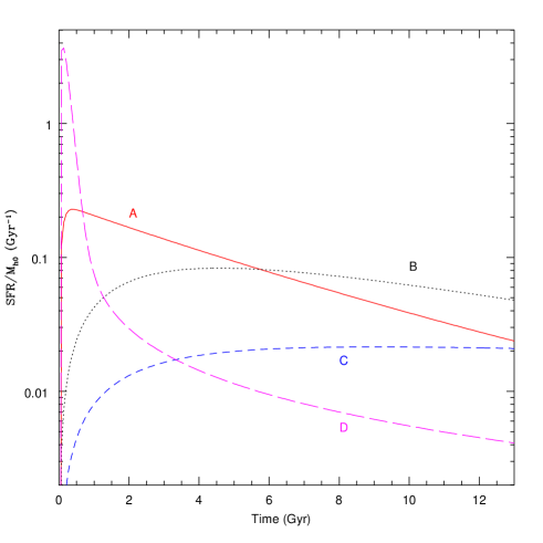
Figure 2: Star formation rates as a function of time for four galaxy models in Table 1. The different curves are meant to represent typical galaxies: model D in Table 1 (long-dashed magenta) belongs to an early-type galaxy, while models B (dotted black) and C (short-dashed blue) are representative of late-type galaxies, and model A (solid red) is a transition galaxy characterized by a short infall timescale and a moderately long star formation rate timescale. The vertical axis gives the SFR normalized by the total mass of the system, $M_{\mathrm{h0}}$ ($M_{\mathrm{h0}}$ is also the mass of the halo at $t=0$ and should be much smaller for irregulars and dwarf ellipticals than for normal-size galaxies).

Table 1: Parameters of some typical galaxy models.

	Pritchet-DTD models				Maoz-DTD models
	A	B	C	D	A’	B’	C’	D’
$\tau_{\mathrm{inf}}$ (Gyr)a	0.1	9.0	50.0	0.1	0.1	9.0	50.0	0.1
$\tau_{\mathrm{sfr}}$ (Gyr)b	4.0	2.0	2.0	0.1	4.0	2.0	2.0	0.1
DTD	P08	P08	P08	P08	M10b	M10b	M10b	M10b
$f_{\mathrm{gas}}$	0.09	0.09	0.04	0	0.09	0.09	0.04	0
$f_{\mathrm{star}}$	0.91	0.67	0.19	1	0.91	0.67	0.19	1
$Z_{\mathrm{host}}$	0.029	0.015	0.012	0.036	0.041	0.022	0.017	0.035
$\Delta\bar{Z}$ (dex)	-0.53	-0.15	-0.089	-0.54	-0.21	-0.047	-0.029	-0.33
$\sigma\left(\Delta\bar{Z}\right)$	0.49	0.19	0.14	0.35	0.39	0.11	0.071	0.41
$X\left(\mathrm{CNO}\right)_{\mathrm{host}}$	0.017	0.0091	0.0076	0.0085	0.017	0.0091	0.0076	0.0085
$\Delta\bar{X}\left(\mathrm{CNO}\right)$ (dex)	-0.48	-0.12	-0.070	-0.13	-0.19	-0.024	-0.017	-0.093
$\sigma\{\Delta\bar{X}\left(\mathrm{CNO}\right)\}$	0.47	0.18	0.13	0.31	0.36	0.10	0.062	0.28

We start by analysing the behaviour of typical galaxies meant to represent from ellipticals to late-type galaxies. Table 1 gives their main parameters together with the final mass fractions of gas and stars with respect to the total mass of the system, the final metallicity (both as given by all metals and by CNO elements) of the host, and the statistical properties of the corresponding MDF of SNIa: metallicity correction and standard deviation of the distribution, $\sigma$. We computed all the model galaxies discussed in this subsection with no outflow. Models A to C are in good agreement with the models in Table 2 of Kobayashi et al. (2000) for galaxies of types E, Sc, and Sd (the remaining mass of gas and the mass of stars at $t=t_{\mathrm{gal}}$ of the models, as well as the final metallicities agree reasonably well given that the model of evolution of the rate of SNIa we use are not the same as their). The SFR of model D is more bursty (Fig. 2), and we include it here as a representative of the early-type galaxy models used in the rest of the paper (even though it has $c_{\mathrm{out}}=0$, which would correspond to a massive early-type galaxy). In this and the next subsection, we present the results obtained with the DTD of P08, while we delay to Section 3.3 the discussion of the differences with respect to the DTD of M10b.

In Fig. 3, we show the distribution of birth-times for a SNIa exploding at $t=t_{\mathrm{gal}}$. The curves peak at the present time because the DTD is strongly biased towards small delay times. This effect is more pronounced in late-type galaxies, for which the star-formation activity is either slightly decreasing or increasing. Early-type galaxies display a similar peak at quite early times, belonging to the epoch of intense star-formation activity, but the importance of this initial peak varies according to the duration of the star-formation epoch. Thus, SNIa from early-type galaxy models come from two different populations whose properties can be quite different: an old, predominantly low-mass, population belonging to the star-formation peak, and a young population characterized by larger masses.

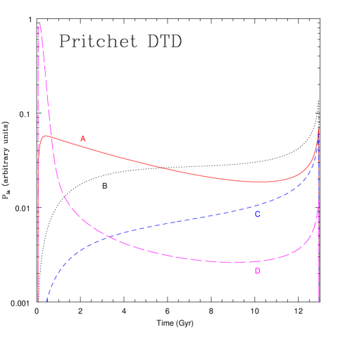
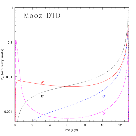
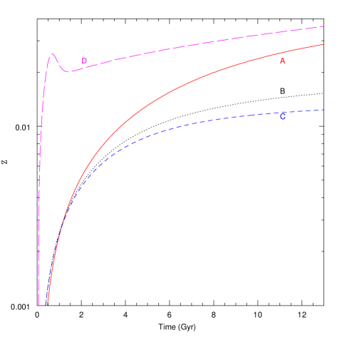
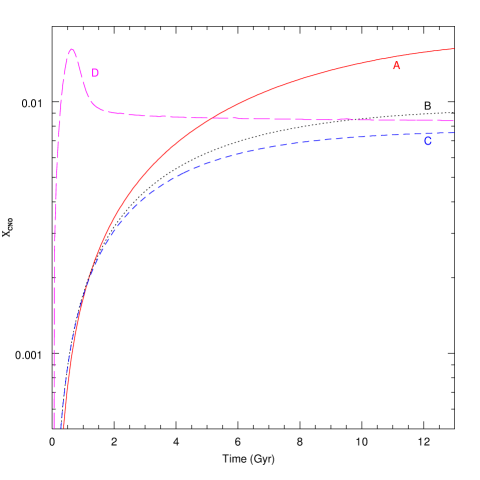
Figure 3: Chemical evolution of the prototypical galaxies (the same models as in Fig. 2 and Table 1). Top row: Probability density that a SNIa exploding at $t=13$ Gyr was born at a given cosmic time obtained with the DTD of P08 (left), and with the DTD of M10b (right). The infall of gas that primes the formation of stars begins at a cosmic time $t=0$ for all the models. Bottom row: Evolution with time of the gas-phase metallicity (left), and the mass fraction of CNO elements (right).

Figure 4 shows the MDF of SNIa, for the same typical galaxies as those in the left panel of Fig. 3, as a function of $\Delta Z$. As can be deduced from Fig. 3, the younger the stellar population of a galaxy is (as in models B and C) the smaller the scatter in metallicity of potential SNIa progenitors. The late-type galaxy distribution is strongly biased towards a zero correction and display a short tail, down to $\Delta Z\sim-0.2$ dex for a galaxy that is still in its initial phases of star formation ($\tau_{\mathrm{inf}}=50$ Gyr, meant to represent an irregular galaxy), and $\Delta Z\sim-0.4$ dex for a galaxy that has already gone through most of the infall process ($\tau_{\mathrm{inf}}=9$ Gyr). The probability of a SNIa metallicity differing in less than 0.1 dex (in absolute value) from $Z_{\mathrm{host}}$ is 75% for the irregular galaxy model and 57% for the model with $\tau_{\mathrm{inf}}=9$ Gyr.

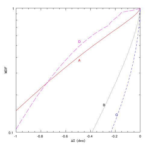
Figure 4: Metallicity distribution function (MDF) of SNIa as a function of the metallicity correction with respect to $Z_{\mathrm{host}}$, for the same models as in the left panel of Fig. 3.

Early-type galaxies show a broader MDF implying that SNIa from these hosts will have a larger intrinsic metallicity dispersion, even if they come from the same host! Again, this behaviour can be understood from the probability density of SNIa progenitors shown in Fig. 3: Models A and D have a substantial contribution of old potential SNIa progenitors, thus they show a large scatter in their MDF. For the model with $\tau_{\mathrm{inf}}=0.1$ Gyr and $\tau_{\mathrm{sfr}}=4$ Gyr half of the SNIa have a metallicity differing more than 0.38 dex (in absolute value) from $Z_{\mathrm{host}}$, while for the model with $\tau_{\mathrm{inf}}=0.1$ Gyr and $\tau_{\mathrm{sfr}}=0.1$ Gyr the median of the correction is -0.49 dex.

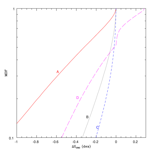
Figure 5: Metallicity distribution function (MDF) of SNIa as a function of the metallicity correction with respect to the host metallicity, but taking the CNO abundance as a measure of metallicity. The models shown are the same as in the left panel of Fig. 3.

Figure 5 shows the MDF of SNIa when the metallicity is measured as the abundance of CNO elements. The main difference with the MDF derived for ’Fe’ is found in the behaviour of the older galaxy model, i.e. the one with $\tau_{\mathrm{inf}}=0.1$ Gyr and $\tau_{\mathrm{sfr}}=0.1$ Gyr. The reason of this behaviour can be understood by looking at Fig. 3 (bottom right panel), where we display the evolution with time of the mass fraction of CNO elements in the gas. The long-dashed (magenta) curve shows the evolution following the short burst of star formation coincident with the infall epoch. Initially the abundance of CNO elements grows fast due to the self-enrichment of the gas due to efficient reprocessing driven by massive stars. Once the star formation burst is over, there are no more massive stars present, and intermediate and low mass stars enrich the interstellar medium at the end of their lifetime with yields representative of their birth time, on average less rich on CNO elements than at the peak of the curve. This causes the CNO abundance to decrease rapidly until it reaches a stable value at about 60% of the peak CNO mass fraction. Therefore, the SNIa that explode at $t=13$ Gyr can have birth metallicites larger than that of the host, as seen in Fig. 5.

Because SNIa are observed at different redshifts, it is also interesting to know if their MDF varies with the elapsed time of galactic evolution, $t_{\mathrm{gal}}$. We have integrated again the evolutionary equations with $t_{\mathrm{gal}}=11$ and 13.7 Gyr. Within this range of $t_{\mathrm{gal}}$ the “metallicity correction“ changes by less than $\sim 10\%$.

3.2 Statistical properties of the SNIa MDF for different types of galaxy

In this section, we use a sample of galactic models with varying $\tau_{\mathrm{sfr}}$, $\tau_{\mathrm{inf}}$, and $c_{\mathrm{out}}$ to study the statistical properties of the relationship between $Z_{\mathrm{Ia}}$ and $Z_{\mathrm{host}}$. We have built models for early-type galaxies by using small values of the timescales associated to infall and SFR: either $\tau_{\mathrm{inf}}=0.1$ Gyr or $0.5$ Gyr, and either $\tau_{\mathrm{sfr}}=0.1$ Gyr or $0.5$ Gyr, and with different degrees of outflow, controlled by the parameter $c_{\mathrm{out}}$. Thus, for each value of $c_{\mathrm{out}}$ we show four models, obtained with the aforementioned combinations of $\tau_{\mathrm{inf}}$ and $\tau_{\mathrm{sfr}}$. In general, the location of these models in the plane $\bar{Z}_{\mathrm{Ia}}$ vs $Z_{\mathrm{host}}$ is driven by $c_{\mathrm{out}}$, while the variation with $\tau_{\mathrm{inf}}$ and $\tau_{\mathrm{sfr}}$ is small.

In order to generate models for late-type galaxies we left the infall and SFR timescales vary in the ranges: $\tau_{\mathrm{inf}}=0.1:60$ Gyr and $\tau_{\mathrm{sfr}}=1:6$ Gyr. In order to avoid too extreme or unrealistic galaxy models we have further constrained our sample to have $0.05\leq f_{\mathrm{gas}}/f_{\mathrm{star}}\leq 3$ and $-0.6\leq\log\left(Z_{\mathrm{host}}/Z_{\odot}\right)\leq 0.5$.

Figure 6 (left panel: DTD of P08) shows the metallicity correction, to be applied to $Z_{\mathrm{host}}$ in order to estimate $Z_{\mathrm{Ia}}$, as a function of the host metallicity. The two kind of galaxies show different behaviour: while there is an approximately linear dependence of the correction on $Z_{\mathrm{host}}$ for late-type galaxies, the correction is about constant for early-type galaxies of every metallicity, i.e. the dispersion of the corrections is much smaller than the range of host metallicities. The linear function that fits the late-type galaxies passes as well through the early-type ones with no outflow ($c_{\mathrm{out}}=0$). As $c_{\mathrm{out}}$ increases, the final metallicities of the early-type hosts decrease while the metallicity correction remains the same.

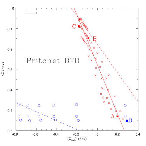
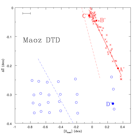
Figure 6: The metallicity correction, i.e. the mean difference between the logarithms of $\bar{Z}_{\mathrm{Ia}}$ and the host metallicity, $Z_{\mathrm{host}}$, as a function of the last. Blue circles represent early-type galaxies, which we have built with small values of the timescales associated to infall and SFR: $\tau_{\mathrm{inf}}=0.1$ and $0.5$ Gyr, and $\tau_{\mathrm{sfr}}=0.1$ and $0.5$ Gyr, and with different degrees of outflow, controlled by the parameter $c_{\mathrm{out}}$. In this and coming figures we have plotted as late-type galaxies (red crosses) all the models with $\tau_{\mathrm{sfr}}\geq 1$ Gyr. The error bar at the top left of each panel is the typical uncertainty in observationally determined $\left[Z_{\mathrm{host}}\right]$ (see Section 3.4). Left: Models computed with the DTD of P08. The solid red line is a linear fit to the data points belonging to late-type galaxies given by: $\Delta\bar{Z}=-1.22\left[Z_{\mathrm{host}}\right]-0.28$, where we have adopted a solar metal fraction $Z_{\sun}=0.01895$. The dashed lines are linear fits belonging to early-type galaxies (blue) and late-type galaxies (red) in the VESPA catalogue computed using the DTD of P08 (see Section 4.2). The filled symbols belong to models C, B, A, and D in Table 1 (from top to bottom). Right: Models computed with the DTD of M10b (note the different range of the vertical axis as compared to the left panel). The solid red line is a linear fit to the data points belonging to late-type galaxies (red crosses), given by: $\Delta\bar{Z}=-0.54\left[Z_{\mathrm{host}}\right]-0.03$. The dashed lines are linear fits belonging to early-type galaxies (blue) and late-type galaxies (red) in the VESPA catalogue computed using the DTD of M10b (see Section 4.2). The filled symbols belong to models C’, B’, A’, and D’ in Table 1 (from top to bottom).

Figure 7 shows the metallicity correction belonging to CNO abundances. It displays the same gross properties as those seen in Fig. 6 with one important difference concerning early-type galaxies: their metallicity corrections are now among the lowest of all models displayed. The reason for this behaviour is again the peculiar MDF of CNO elements in SNIa from this kind of galaxies as seen in Fig. 5. The dispersion of their MDF is, however, similar to that of galaxies with a much larger metallicity correction (compare models A and D in Table 1).

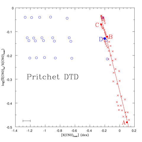
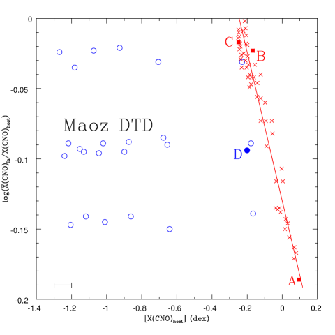
Figure 7: The metallicity correction with respect to the gas-phase metallicity of the host, when the metallicity is measured as the CNO abundance. The error bar at the bottom left of each panel is the typical uncertainty in observationally determined $\left[X(\mathrm{CNO})_{\mathrm{host}}\right]$ (see Section 3.4). Left: Models computed with the DTD of P08 (note the different range of the vertical axis as compared to the left panel). The straight line is a linear fit to the data points belonging to late-type galaxies (red crosses), given by: $\overline{\log}\left(X(\mathrm{CNO})_{\mathrm{Ia}}/X(\mathrm{CNO})_{\mathrm{host}}\right)=-1.24\left[X(\mathrm{CNO})_{\mathrm{host}}\right]-0.35$, where we have adopted a solar CNO mass fraction $X(\mathrm{CNO})_{\sun}=0.0134$. From top to bottom, the filled circles belong to models C, B, D, and A in Table 1. Right: Models computed with the DTD of M10b. The straight line is a linear fit to the data points belonging to late-type galaxies (red crosses), given by: $\overline{\log}\left(X(\mathrm{CNO})_{\mathrm{Ia}}/X(\mathrm{CNO})_{\mathrm{host}}\right)=-0.53\left[X(\mathrm{CNO})_{\mathrm{host}}\right]-0.19$. From top to bottom, the filled circles belong to models C’, B’, D’, and A’ in Table 1.

In many observational studies, it is necessary to generate a random set of SNIa with stochastic metallicities in order to compare their statistical properties with those of the observational sample. The linear fit of $\Delta\bar{Z}$ vs. $[Z_{\mathrm{host}}]$ shown in Fig. 6 together with the MDF may be used to generate such a random set of SNIa, with stochastic metallicities related (but not equal) to their host metallicities. The simpler way to do this is to approximate the MDF of SNIa as a straight line in the semi-logarithmic plot shown in Fig. 4,

$$\log(\mathrm{MDF})=\alpha\Delta Z\,,$$ (22)

that determines the probability density,

$$P^{\prime}(\Delta Z)=\alpha\exp\left(\alpha\Delta Z\right)\,,$$ (23)

the mean metallicity correction,

$$\Delta\bar{Z}=-1/\alpha\,,$$ (24)

and the standard deviation, $\sigma$, of the distribution of $\Delta Z$:

$$\sigma=1/\alpha=-\Delta\bar{Z}\,.$$ (25)

In Table 1 we give the standard deviation of the MDF of our typical galaxy models. As can be seen, the relationship between $\Delta\bar{Z}$ and $\sigma$ derived in Eq. 25 approximately holds for all the models, with the exception of the distribution of CNO in models D and D’, for which a simple proportionality law as that of Eq. 22 is not a good fit (see Fig. 5).

To generate a stochastic distribution of SNIa metallicites in a late-type galaxy of known $Z_{\mathrm{host}}$, one would have first to apply the linear function of Fig. 6 (or that in Fig. 7 if what is desired is the distribution of mass fractions of the CNO elements) to obtain the metallicity correction $\Delta\bar{Z}$ and $\sigma$ ($=-\Delta\bar{Z}$). For an early-type host the procedure is even simpler, as the metallicity correction takes on a nearly constant value for this kind of galaxies.

3.3 Choice of the Delay Time Distribution

The Delay Time Distribution is a property specific of SNIa that has rather small imprint on the galactic chemical evolution of CNO elements but affects strongly the temporal distribution of SNIa, hence it is expected to influence appreciably the MDF. The DTD of SNIa is a matter of current debate (Strolger et al., 2004; Scannapieco & Bildsten, 2005; Greggio, 2005; Greggio et al., 2008; Maoz et al., 2010a). P08 proposed a model in which the rate of SNIa was proportional to the WD formation rate. This model reproduced satisfactorily the trend of SNIa rates as a function of the specific SFR in galaxies of ages between 1 and 13 Gyr. In a recent work, Maoz et al. (2010a) presented a method to recover the supernova DTD that simultaneously takes into account supernova data and the reconstructed star formation history of the individual galaxies in a survey, and applied this method to the events present in the LOSS SN survey and in the VESPA database. Independently, Brandt et al. (2010) analyzed light curves and host galaxy spectra of 101 SNIa from the SDSS using VESPA algorithms, from which they derived the DTD of SNIa. Maoz et al. (2010a) found that their data required a stronger short delay-time component than allowed by the model of P08, i.e. they called for a higher contribution from large mass progenitors. The VESPA database is organized in temporal bins, whose resolution is better at the present epoch and degrades with look-back time (for further details see Section 4), hence the results of Maoz et al. (2010a) should be more sensitive to the short delay time component of the SNIa DTD. Thus, the discrepancy between the models proposed by P08 and Maoz et al. (2010a) might be due to the different sensitivities to the time ranges of the SNIa DTD (but see M10b). Anyway, it is necessary to check the imprint that the different DTD have on the MDF of SNIa.

Having used a model based on P08 in the previous sections, we now discuss the results obtained with the DTD of M10b, Eq. 13 in their paper,

$$\Psi(t)=0.7\times 10^{-3}t^{s}\,\mathrm{SN}~{}\mathrm{M}_{\odot}^{-1}~{}\mathrm{Gyr}^{-1}\,,$$ (26)

where $s=-1.2$, $t$ is measured in Gyr, and we have applied a factor 0.7 to the DTD of M10b to convert back from their ’diet-Salpeter’ IMF to ours. Models A’ to D’ in Table 1 were computed using their DTD in Eqs. 4 and 5. The right panel of Fig. 3 shows the distribution of birth-times for a SNIa exploding at $t=t_{\mathrm{gal}}$ for these model galaxies. With respect to the DTD of P08 (left panel of Fig. 3) the new DTD increases the contribution from young stars (small delay-time) with respect to old stars. Late-type galaxies are scarcely affected at all, but early-type galaxies display a quite different trend in which the contribution of the population belonging to the initial star-formation peak is dramatically reduced. With this new DTD, the differences between galaxy-types strongly smooth out.

The metallicity correction obtained with the DTD of M10b is shown in the right panel of Figs. 6 and 7, for both late-type and early-type galaxies. Overall, the correction is significantly smaller than that obtained using the DTD of P08, as expected given the larger contribution from prompt SNIa implied by the DTD of M10b.

From these results it is clear that the DTD of SNIa is the most important factor determining the magnitude of the correction needed to obtain the metallicity of SNIa from those of their host galaxies. We stress that any of the above DTD models (P08 vs. M10b) is subject to a large degree of observational uncertainty. For instance, M10b discuss two possible approaches to determine the power law exponent in Eq. 26, based on what they call the ’optimal-iron constraint’ and the ’minimal-iron constraint’, which lead to different exponents, $s$, in the range from -1.5 to -0.9 (in this study, we have adopted in Eq. 26 the mean, i.e. -1.2). It is interesting to consider how much would change the plots in Figs.  6 and 7 if $s$ covered the full range given by M10b. We have repeated the calculations with $s=-1.5$ and $s=-0.9$. For the first case, belonging to an extreme case of the ’optimal-iron constraint’, the straight-line fit to our late-type galaxies changes to $\Delta\bar{Z}=-0.28\left[Z_{\mathrm{host}}\right]+0.06$ while the correction for early-type galaxies changes by $\sim+0.12$ dex. For the last case, belonging to an extreme case of the ’minimal-iron constraint’, the fit of the late-type host corrections changes to $\Delta\bar{Z}=-0.89\left[Z_{\mathrm{host}}\right]-0.16$, and the corrections for early-type hosts changes by $\sim-0.04$ dex. We can see that the uncertainty in the DTD leads to uncertainties in $\Delta\bar{Z}$ of the same order as the own correction. We conclude that an accurate determination of the DTD of SNIa is a prerequisite to achieve a good understanding of the differences between the metallicities of these supernovae and those of their host galaxies.

3.4 Is it the host metallicity a good estimator of the SNIa metallicity?

Here we discuss the reliability of different host metallicity estimators as for establishing the statistical properties of SNIa: gas-phase vs. stellar metallicity, $Z_{\mathrm{star}}$, and gaseous CNO abundance vs. Fe abundance.

We have evaluated the mean host stellar metallicity as the mean of the metallicity of the ISM at star birth, weighted by the SFR and by the IMF, for all the stars whose mean-sequence lifetime is larger than the elapsed time since their formation. The mean stellar metallicity derived by observational studies is weighted by the contribution of stars in different phases of their life, with weights depending on the particular spectral feature used for measuring the metallicity. Even though both ways to define a mean stellar metallicity may give different values, we expect that both will follow the same qualitative trends.

Fig. 8 shows the metallicity correction to apply if the host galaxy metallicity is measured from the stellar population (and the DTD of M10b is used). In comparison with the trend shown in the right panel of Fig. 6 we notice that the corrections to apply to the metallicities of early-type galaxies continues being independent of host metallicity, but now they cluster around $\Delta\bar{Z}=0$. Late-type galaxies display also a similar behaviour as in Fig. 6, with changed sign, but they could not be fitted by a linear function and show larger dispersion for given $Z_{\mathrm{host}}$. Thus, if possible, it is advisable to measure the metallicity of SNIa in late-type hosts as that of their gas. These results can be understood by computing the distribution of birth-times of present-day (at $t=t_{\mathrm{gal}}=13$ Gyr) stars. We have calculated the distribution of birth times as the fraction of the mass in present-day stars represented by the stars born at time $t$ that are still alive,

$$\frac{\mathrm{d}m_{\mathrm{star}}}{\mathrm{d}t}=S(t)\int_{M_{\mathrm{bot}}}^{M(t_{\mathrm{gal}}-t)}\phi(M)M\mathrm{d}M\,.$$ (27)

The distribution of birth-times follows closely the SFR of each model (see Fig. 2) because 99% of the stellar mass at birth belongs to stars smaller than $\sim 0.5$ M_⊙ (for our Salpeter IMF), hence the integral in Eq. 27 is always close to $\sim 1$. Comparing Fig. 2 with the probability density of birth times of SNIa shown in Fig. 3 (top right) it is easy to see that the average age of SNIa progenitors is much less than the average age of the stellar population, especially because the peak of $P_{\mathrm{Ia}}$ at times close to $t_{\mathrm{gal}}$. In galaxies characterized by a monotonic increase of the metallicity (models A’, B’, and C’) the immediate consequence is that the metallicity of SNIa is larger than the average stellar metallicity. Early-type galaxies, like model D’, display a non-monotonic evolution of the metallicity, that peaks later than the SFR. For instance, for model D’ the peak of the SFR occurs at $t\simeq 0.1$ Gyr, while the peak of $Z_{\mathrm{gas}}$ is found at $\sim 0.85$ Gyr and that of $X_{\mathrm{CNO}}$ takes place at $\sim 0.60$ Gyr. Thus, the stellar population is chiefly drawn from low-metallicity gas, while SNIa have an appreciable contribution from times close to present, at which the gas metallicity is much larger.

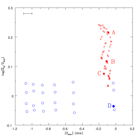
Figure 8: The metallicity correction, taking as a reference the mean stellar metallicity, $Z_{\mathrm{star,}}$, instead of the gas metallicity, $Z_{\mathrm{host}}$. Here we have used the DTD of M10b. The filled symbols belong to models A’, B’, C’, and D’ in Table 1 (from top to bottom). The error bar at the top left of the figure is the typical uncertainty in observationally determined $\left[Z_{\mathrm{star}}\right]$ (see discussion at the end of Section 3.4).

In Fig. 7 we show the metallicity correction when the gas-phase metallicity is estimated from the mass fraction of CNO elements in the gas. In comparison with Fig. 6 the CNO metallicity correction is nearly identical to the Fe correction for late-type galaxies but significantly smaller for early-type hosts, for a given DTD. As can be seen in Fig. 3 (bottom row) the chemical evolutions of Fe and CNO elements in the galaxy models A’, B’, and C’ are in close agreement, thus the MDF of both element groups are similar (compare Fig. 4 with Fig. 5). Thus, the use of Fe instead of CNO abundances does not seem to represent an improvement in the estimates of SNIa metallicities obtained from those of their hosts. The host CNO abundance of early-type galaxies is in much better agreement with the mean SNIa one than are the corresponding total metal abundances, although their dispersions are similar. Using again the chemical evolution computed for the prototypical galaxy model D’, displayed in the bottom row of Fig. 3, and the probability density of SNIa shown in Fig. 3, the reason for this closer agreement between CNO abundances in SNIa and the gas, as compared with Fe abundances, is that SNIa from early-type galaxies have non-negligible contributions from quite early times and near present time. The CNO abundances are low at both times, because presently there are no high-mass stars contributing to their synthesis. On the other hand, the Fe abundance increases continuously during the last 11 Gyr due to the contribution of SNIa, with the result that young SNIa progenitors are drawn from gas with high Fe abundance while old SNIa progenitors were born from gas with quite small Fe abundance. Hence, the average discrepancy between present-day gas Fe abundance and that of SNIa is larger than in the case of the CNO abundances.

A meaningful evaluation of the corrections we propose to obtain SNIa metallicities from the different metallicity measures of their hosts can only be done by considering the observational errors in the galactic metallicity and in the DTD of SNIa. As discussed in the Introduction, galactic metallicities are measured using different methods, all of them subject to a suite of experimental and theoretical uncertainties. Gallagher et al. (2008) measured the Fe abundance of the gas of early-type hosts of SNIa with quite different errors, depending on the host. An average error in $\left[Z_{\mathrm{host}}\right]$ of 0.1-0.2 dex can be deduced from their Table 4 and from the comparison they perform with metallicities measured by Trager et al. (2000) and Thomas et al. (2005) for a subset of galaxies they have in common. On the other hand, the Tremonti et al. (2004) mass-metallicity relationship, used by Howell et al. (2009) to measure host metallicity, is sensitive to $\left[\mathrm{O}/\mathrm{H}\right]$ in the gas phase. The scatter in this relationship is of order $\sim 0.1$ dex. Finally, the observational determination of $\left[Z_{\mathrm{star}}\right]$ is subject to systematic biases of order $0.1-0.2$ dex (Cid Fernandes et al., 2005). Summarizing, the uncertainty in the measured metallicity of SNIa hosts is similar for the different metallicity tracers, $\epsilon\sim 0.1$ dex, although it may be substantially larger for a given galaxy.

We have drawn in Figs. 6, 7, and 8 an error bar indicative of the typical uncertainty in the measured host metallicity. These uncertainties are not large compared to the range of host metallicities covered in the figures (horizontal axes). One can also compare the host metallicity uncertainty with the correction necessary to obtain $Z_{\mathrm{Ia}}$, plotted in the same figures (vertical axes). Looking at the corrections deduced for the DTD of P08 (left panels of the same figures) it can be seen that they are in general much larger than $\epsilon$. On the contrary, if the DTD of M10b is used (right panels of Figs. 6 and 7), $\Delta\bar{Z}_{\mathrm{Ia}}$ is of the same order as $\epsilon$, especially for early-type galaxies. Thus, if this last DTD were the correct choice, the error in the determination of SNIa metallicity would be dominated by the uncertainty in the measurement of the host metallicity rather than the difference between galactic and supernova metallicities.

4 Exploiting galactic databases

In this section, we explore the facilities provided by current galactic catalogues in order to obtain observational constraints to our theoretically derived MDF of SNIa. Ideally, one might use an observationally determined star formation history (SFH) of a galaxy together with a gas metallicity history, determined through metallicity-dependent synthetic stellar population (SSP) models, to recover a probability distribution function for the metallicity of SNIa progenitors. In practice, however, there are limitations due to both the discretisation of the catalogue in time bins of finite size, and the paucity of metallicities used in the SSP models. In Section 4.1 we shortly address how to reformulate Eqs. 7 and 8 in order to calculate the probability that a SNIa progenitor was born in a given time bin. We apply then the new formalism to the VESPA catalogue, and discuss the results and the consequences of the paucity of metallicities in the SSP models in Section 4.2. We explain the main characteristics of the VESPA catalogue in the next paragraph.

VESPA (’VErsatile SPectral Analysis’, Tojeiro et al., 2007) is a method to reconstruct star formation and metallicity histories from galactic spectra using SSP models. Tojeiro et al. (2009) applied their VESPA code to all galaxy spectra in the seventh data release of the SDSS (York et al., 2000), and compiled their results in a publicly accessible catalogue of stellar masses, star formation rates and metallicity histories of nearly 800,000 galaxies . VESPA uses all of the available absorption features and the shape of the continuum (emission lines are not included in the analysis) in order to estimate the SFH of each galaxy, with variable time resolution, and the metallicity of the stars born in each time bin, which traces the gas metallicity. The number of time bins depends on the quality of the data on each galaxy. At the highest resolution, VESPA uses 16 age bins, logarithmically spaced between look-back times 0.002 Gyr and 13.7 Gyr, however if the data are not of sufficient quality some bins may lack information. The VESPA catalogue contains results from several runs using different SSP models, IMF prescriptions, dust models, and galactic samples (for details see the above-mentioned papers from Tojeiro et al). The SSP models are supplied at metallicities of $Z=0.0004$, 0.01, 0.02, and 0.04.

4.1 Probability that a SNIa originated in a given time interval

The present rate of SNIa explosions in a given host is the convolution over time of the SFR and the DTD. The probability that a SNIa that explodes now (at time $t$) comes from a progenitor born at time $t^{\prime}=t-\tau$ is given by Eq. 5. Assuming we know the DTD and that the SFR can be obtained from a galactic catalogue, both in discrete time bins, the probability that the SNIa was born at time bin $i$ is (for a given galaxy):

$$P_{i}=\frac{\Psi_{i}\mathcal{M}_{i}}{\sum\Psi_{j}\mathcal{M}_{j}}\,,$$ (28)

where the addition in the denominator extends to all bins defined for that galaxy, and $\mathcal{M}_{i}$ is the mass of stars formed in time bin $i$.

If the observational DTD is not known with enough resolution (as compared to the time bin resolution in a given catalogue), one can turn to the model of P08 (Eq. 7) or its equivalent based on the DTD of M10b (Eq. 8). What we actually need in order to use the galactic catalogue is the probability that a SNIa exploding now comes from a progenitor born within a time interval given by the temporal bins defined in the catalogue: say between look-back times $\tau_{i}$ and $\tau_{i}+\Delta t_{i}$:

$$P_{i}\propto\int_{\tau_{i}}^{\tau_{i}+\Delta t_{i}}S(t-t^{\prime})\phi(M_{t^{\prime}})\left(\frac{dM}{dt}\right)_{t^{\prime}}dt^{\prime}\,,$$ (29)

where we have used the DTD of P08. To use the catalogued data we transform the above integral using a mean SFR defined from the stellar mass formed in the time interval $i$ and the duration of that time interval, $\Delta t_{i}$: $\bar{S}_{i}=\mathcal{M}_{i}/\Delta t_{i}$, and combine $(dM/dt)dt^{\prime}=dM$:

$$P_{i}\propto\frac{\mathcal{M}_{i}}{\Delta t_{i}}\int_{M(\tau_{i}+\Delta t_{i})}^{M(\tau_{i})}\phi(M)dM\,.$$ (30)

The integral in the last equation can be easily computed given the IMF, the stellar lifetime law, and the temporal limits of each bin. Note that there is no need to know the proportionality constant for $P_{i}$ nor even to re-normalize the IMF, because we know that $\sum P_{i}=1$, if we add $P_{i}$ for all the bins in a galaxy. Thus, the probability density can be normalized unambiguously.

If the DTD of M10b is adopted instead, $P_{i}$ can be obtained from:

$$P_{i}\propto\frac{\mathcal{M}_{i}}{\Delta t_{i}}\bar{\Psi}\,,$$ (31)

where $\bar{\Psi}$ is the average DTD between $\tau_{i}$ and $\tau_{i}+\Delta t_{i}$.

From the previously determined probability that a SNIa comes from time bin $i$, $P_{i}$, and the catalogued metallicity for that same time bin, $Z_{i}$, the metallicity probability density is given by:

$$P^{\prime}(\Delta Z)=P^{\prime}(\log Z_{i}-\log Z_{host})=P_{i}\,.$$ (32)

This procedure provides us with a discrete set of $\Delta Z$ for which the probability density is known.

4.2 Results using VESPA: dependence on the star formation rate and host age

Here we show an example of the application of the formalism introduced in the last Section to real data. We have accessed the VESPA catalogue (runID=2) and classified the galaxies as early or late-type according to the criterion proposed by Dilday et al. (2010) on base of their $u$ and $r$ SDSS model magnitudes. Then, we have selected the galaxies with a minimum temporal resolution of three bins, in order to work with reasonable SFHs. Finally, we recovered 90 906 early-type galaxies and 40 419 late-types. We stress that we have not filtered the catalogue in order to select which galaxies are potential SNIa hosts. From a theoretical point of view, every single galaxy can house binaries with the appropriate parameters (total mass, secondary mass, initial separation, metallicity) to produce SNIa. Observationally it is another story, because surveys aiming to detect SNIa have to pre-select target galaxies for which the observations and measurements are more efficient. This difference has to been kept in mind when comparing between our theoretically derived SNIa statistics and the correlations found in observational campaigns.

We have applied the formalism developed in the previous section (Eqs. 31 and 32) to all the galaxies selected from VESPA in order to obtain the MDF of each galaxy. Unfortunately, at the present level of resolution of the catalogue the resulting MDF is of little practical use because of the limited spectra of metallicities of the SSP models. As the MDF is an statistical description of the difference of metallicity between the host and the SNIa, the use of just four metallicities in the SSP models produces an unreliable extremely clumpy MDF. Keeping this in mind, we comment here briefly on the relationship between the metallicity correction, $\Delta\bar{Z}$, and the $Z_{\mathrm{host}}$ obtained from the catalogue. Linear fits to these quantities are shown as dashed lines in Fig. 6. Given the uncertainties, it is striking the close coincidence between the points belonging to our theoretical models and the linear fits obtained with the catalogue, especially for late-type galaxies. The differences between theoretical models of early-type and late-type galaxies are more or less reproduced by the mean metallicities derived from VESPA.

In view of the strong uncertainty affecting the metallicity statistics, we do not follow further with the analysis of the VESPA derived MDF, but we emphasize that the formalism presented in the previous subsection can (and should) be applied to future galactic catalogues based on improved data and metallicity resolution. In spite of the failure to derive useful MDF from VESPA, the data from the catalogue can still be used to show trends of the mean SNIa metallicity, $\bar{Z}_{\mathrm{Ia}}$ calculated using the probability defined by Eq. 31, vs. the galactic SFR and age.

Figure 9 shows $\bar{Z}_{\mathrm{Ia}}$ as a function of the sSFR (specific Star Formation Rate). We first notice the sharp cut on top of the points distribution at $\bar{Z}_{\mathrm{Ia}}=0.4$, which derives from the maximum metallicity fed to the SSP models of VESPA. If we disregard this limitation of the models, we can still fit a tendency line to the data points, with the result that can be seen in the plot: SNIa exploding in high sSFR galaxies do have smaller $\bar{Z}_{\mathrm{Ia}}$ than those that explode in passive galaxies. On the other hand, the tendency lines for early and late-type galaxies do not differ significantly. While the correlation is not strong, we note that a relationship between sSFR and SNIa luminosity has been found in some observational studies of SNIa (e.g., to cite just one, Sullivan et al., 2010, who found that SNIa in low sSFR galaxies appear brighter on average than those in high sSFR galaxies, after applying stretch corrections). As a note of caution, we remark that our galaxy sample was drawn from the whole unfiltered VESPA catalogue whereas each observational study of SNIa properties are based on particular selection function of hosts. Thus, a direct comparison with our results might not be meaningful.

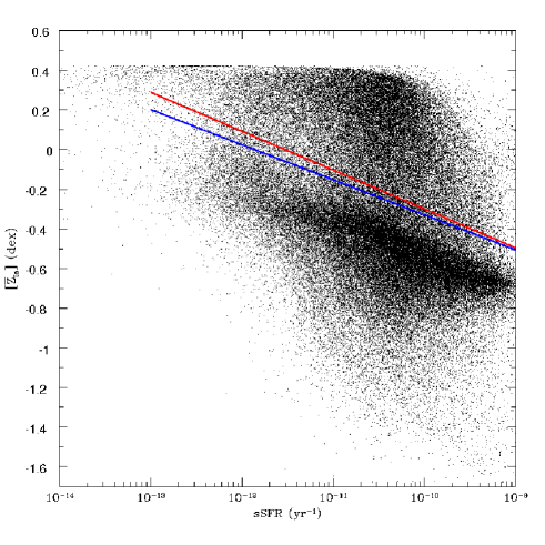
Figure 9: Mean $\bar{Z}_{\mathrm{Ia}}$ as a function of the specific SFR, as derived from the VESPA catalogue (runID=2) and the DTD of M10b. The solid lines are the results of linear fits to the points given by $[\bar{Z}_{\mathrm{Ia}}]=-0.177\log\left(\mathrm{sSFR}\right)-2.10$ (blue, early-type galaxies) and $[\bar{Z}_{\mathrm{Ia}}]=-0.196\log\left(\mathrm{sSFR}\right)-2.26$ (red, late-type galaxies).

Figure 10 shows the distribution of $\bar{Z}_{\mathrm{Ia}}$ as a function of the look-back time of the host galaxy (that is: $t_{\mathrm{back}}=d/c$, where $d$ is the distance to the galaxy and $c$ is the speed of light), that is itself a measure of the age of the universe at the local host time, and of the redshift. Besides the accumulation of points around $Z=0.04$, the data show a tendency for smaller $\bar{Z}_{\mathrm{Ia}}$ at lower redshift. The trend of $Z_{\mathrm{host}}$ with look-back time (not shown in the Fig.) is opposite to that of $\bar{Z}_{\mathrm{Ia}}$, i.e. older hosts are less metal-rich as expected from popular galaxy evolution models. The sign of the slope of $\bar{Z}_{\mathrm{Ia}}$ vs. $t_{\mathrm{back}}$ is difficult to explain, as it implies that SNIa are on average less luminous at high redshifts, contrary to what is derived from observational samples (e.g. Howell et al., 2009, their Fig. 8). Anyway, we cannot derive any strong conclusion given the limitations of the present analysis, as the trend we detect might be a result of observational biases of the catalogued data.

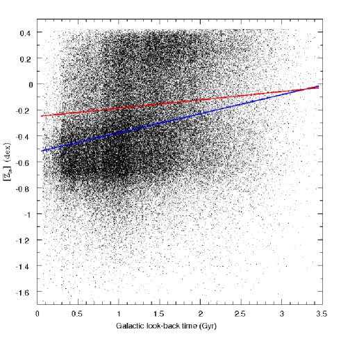
Figure 10: Mean $\bar{Z}_{\mathrm{Ia}}$ as a function of the look-back time of the host galaxy, $t_{\mathrm{back}}$, derived from the VESPA catalogue (runID=2) and the DTD of M10b. The solid lines are the results of linear fits to the points given by $[\bar{Z}_{\mathrm{Ia}}]=0.147t_{\mathrm{back}}-0.524$ (blue, early-type galaxies) and $[\bar{Z}_{\mathrm{Ia}}]=0.064t_{\mathrm{back}}-0.251$ (red, late-type galaxies).

We have checked that the above trends are qualitatively independent of the assumptions concerning the DTD and the specific runs of VESPA that can be selected (galactic samples, SSP models, IMF prescriptions, and dust models). We have also tested the scatter of the parameters of the tendency lines in Figs. 9 and 10 as a result of the uncertainties in the galactic properties stored in the catalogue (errors in the metallicity and star formation rates in each galactic bin). To this end, we have computed again the tendency lines for 200 random realizations of the galactic sets (early-types and late-types) by adding random noise according to the catalogued metallicity and SFR errors in every time bin of each galaxy of our VESPA sample. For each random realization, we have computed the tendency line and thereafter we have analyzed the distribution of slopes, their mean and standard deviation. The standard deviation of the slope of the tendency lines of sSFR and $t_{\mathrm{back}}$ with respect to $\bar{Z}_{\mathrm{Ia}}$ is typically less than 0.002.

5 Conclusions

We have calculated the chemical evolution of homogeneous galaxy models together with the evolution of the supernova rates in order to evaluate the Metallicity Distribution Function of SNIa, $\mathrm{MDF}(\Delta Z)$, i.e. the probability that the logarithm of the metallicity of a SNIa exploding now differs in less than $\Delta Z$ from that of its host. We have analysed several model galaxies aimed to represent from active to passive galaxies, including dwarf galaxies prone to experience supernova driven outflows.

Our results show a remarkable degree of coincidence (in an statistical sense) between the mean $Z_{\mathrm{Ia}}$ and $Z_{\mathrm{host}}$. The dispersion of $Z_{\mathrm{Ia}}$ in active galaxy models is quite small, meaning that $Z_{\mathrm{host}}$ is a quite good estimator of the supernova metallicity, while passive galaxies present a larger dispersion. We have devised a procedure to correct the difference in metallicity between SNIa and their hosts (Sect. 3.2), based on a linear fit given in Fig. 6. These results are insensitive to the choice of IMF, stellar lifetime and stellar yields, within the ranges we have explored. In contrast, the Delay Time Distribution of SNIa remains one of the main ingredients influencing the difference of metallicity between SNIa and their hosts.

We have discussed the use of different metallicity indicators (Fe vs. O, gas-phase metallicity vs. stellar metallicity). Using O (assuming its evolution is representative of that of the CNO group) as a metallicity measure for late-type galaxies does not change appreciable the metallicity correction with respect to using Fe (assuming its evolution is representative of that of all metals). It is remarkable that the metallicity correction for early-type galaxies ($\tau_{\mathrm{sfr}}<1$ Gyr) is quite different for O than for Fe. On the other hand, the metallicities of SNIa are much better represented by those of the gas-phase than by the mean stellar metallicities. Thus, when possible, it is advisable to measure the host metallicity through that of its gas-phase.

Finally, the results of the application of our formalism to a galactic catalogue (VESPA) suggest that SNIa come, in average, from smaller metallicity progenitors both at low redshifts and in galaxies with large star-formation activity. The paucity of metallicities used in the original stellar-population synthesis models used in the construction of the galactic catalogue does not allow us to build a significant MDF of SNIa based on the galactic histories stored in the database. However, in spite of the large uncertainty in the metallicity derived from the catalogue, the gross trends of $\bar{Z}_{\mathrm{Ia}}$ vs. $Z_{\mathrm{host}}$ obtained from VESPA for different galaxy types are roughly consistent with our theoretical estimates. The derivation of improved, observationally based, MDF will be possible in the future if the SSP models include further refinements in their grid of metallicities.

One of the main drawbacks of our approach is the use of homogeneous one-zone galactic chemical evolution models. Actual galaxies are heterogeneous, and radial gradients of chemical composition are routinely measured within them. A possible improvement of our model would be to divide the galaxy in several non-interacting shells as in, e.g., Martinelli et al. (1998), then computing the galactic MDF accounting for the probability that a SNIa originates in each shell. Then, however, a complication would arise when comparing to observations of far away galaxies for which there is no possibility of measuring the metallicity gradient: what is the meaning of the galaxy metallicity in a context where each independent shell has its own chemical history? What is clear is that the derived MDF of SNIa would be characterized by a larger dispersion than the MDF we have obtained. In some sense, the true MDF of SNIa reflects a double dependence: in space, i.e. the position of the SNIa progenitor within its host galaxy, and in time, i.e. the moment in the galactic history when the progenitor was born. It is just this last dependence what we have studied in the present work.

References

- Arimoto & Yoshii (1987) Arimoto, N. & Yoshii, Y. 1987, A& A, 173, 23
- Badenes (2010) Badenes, C. 2010, Proceedings of the National Academy of Science, 107, 7141
- Badenes et al. (2008) Badenes, C., Bravo, E., & Hughes, J. P. 2008, ApJ, 680, L33
- Badenes et al. (2009) Badenes, C., Harris, J., Zaritsky, D., & Prieto, J. L. 2009, ApJ, 700, 727
- Badenes et al. (2010) Badenes, C., Maoz, D., & Draine, B. T. 2010, MNRAS, 969
- Baugh et al. (1998) Baugh, C. M., Cole, S., Frenk, C. S., & Lacey, C. G. 1998, ApJ, 498, 504
- Binney & Merrifield (1998) Binney, J. & Merrifield, M. 1998, Galactic astronomy, ed. Binney, J. & Merrifield, M.
- Brandt et al. (2010) Brandt, T. D., Tojeiro, R., Aubourg, É., et al. 2010, AJ, 140, 804
- Bravo et al. (2010) Bravo, E., Domínguez, I., Badenes, C., Piersanti, L., & Straniero, O. 2010, ApJ, 711, L66
- Buzzoni (2002) Buzzoni, A. 2002, AJ, 123, 1188
- Catalán et al. (2009) Catalán, S., Isern, J., García-Berro, E., & Ribas, I. 2009, Journal of Physics Conference Series, 172, 012007
- Chabrier (2003) Chabrier, G. 2003, PASP, 115, 763
- Cid Fernandes et al. (2005) Cid Fernandes, R., Mateus, A., Sodré, L., Stasińska, G., & Gomes, J. M. 2005, MNRAS, 358, 363
- Conroy et al. (2009) Conroy, C., Gunn, J. E., & White, M. 2009, ApJ, 699, 486
- Cooper et al. (2009) Cooper, M. C., Newman, J. A., & Yan, R. 2009, ApJ, 704, 687
- Dilday et al. (2010) Dilday, B., Bassett, B., Becker, A., et al. 2010, ApJ, 715, 1021
- Domínguez et al. (2001) Domínguez, I., Höflich, P., & Straniero, O. 2001, ApJ, 557, 279
- Ellis et al. (2008) Ellis, R. S., Sullivan, M., Nugent, P. E., et al. 2008, ApJ, 674, 51
- Gallagher et al. (2005) Gallagher, J. S., Garnavich, P. M., Berlind, P., et al. 2005, ApJ, 634, 210
- Gallagher et al. (2008) Gallagher, J. S., Garnavich, P. M., Caldwell, N., et al. 2008, ApJ, 685, 752
- Gavazzi et al. (2002) Gavazzi, G., Bonfanti, C., Sanvito, G., Boselli, A., & Scodeggio, M. 2002, ApJ, 576, 135
- Greggio (2005) Greggio, L. 2005, A& A, 441, 1055
- Greggio & Cappellaro (2009) Greggio, L. & Cappellaro, E. 2009, in American Institute of Physics Conference Series, Vol. 1111, American Institute of Physics Conference Series, ed. G. Giobbi, A. Tornambe, G. Raimondo, M. Limongi, L. A. Antonelli, N. Menci, & E. Brocato, 477–484
- Greggio et al. (2008) Greggio, L., Renzini, A., & Daddi, E. 2008, MNRAS, 388, 829
- Hamuy et al. (2000) Hamuy, M., Trager, S. C., Pinto, P. A., et al. 2000, AJ, 120, 1479
- Hartwick (1976) Hartwick, F. D. A. 1976, ApJ, 209, 418
- Howell et al. (2009) Howell, D. A., Sullivan, M., Brown, E. F., et al. 2009, ApJ, 691, 661
- Kasen et al. (2009) Kasen, D., Röpke, F. K., & Woosley, S. E. 2009, Nature, 460, 869
- Kauffmann & Charlot (1998) Kauffmann, G. & Charlot, S. 1998, MNRAS, 294, 705
- Kelly et al. (2010) Kelly, P. L., Hicken, M., Burke, D. L., Mandel, K. S., & Kirshner, R. P. 2010, ApJ, 715, 743
- Kobayashi & Arimoto (1999) Kobayashi, C. & Arimoto, N. 1999, ApJ, 527, 573
- Kobayashi et al. (2000) Kobayashi, C., Tsujimoto, T., & Nomoto, K. 2000, ApJ, 539, 26
- Kobayashi et al. (2006) Kobayashi, C., Umeda, H., Nomoto, K., Tominaga, N., & Ohkubo, T. 2006, ApJ, 653, 1145
- Kroupa (2007) Kroupa, P. 2007, ArXiv Astrophysics e-prints
- Larson (1974) Larson, R. B. 1974, MNRAS, 169, 229
- Lentz et al. (2000) Lentz, E. J., Baron, E., Branch, D., Hauschildt, P. H., & Nugent, P. E. 2000, ApJ, 530, 966
- Maoz et al. (2010a) Maoz, D., Mannucci, F., Li, W., et al. 2010a, ArXiv e-prints
- Maoz et al. (2010b) Maoz, D., Sharon, K., & Gal-Yam, A. 2010b, ApJ, 722, 1879
- Martinelli et al. (1998) Martinelli, A., Matteucci, F., & Colafrancesco, S. 1998, MNRAS, 298, 42
- Matteucci (2008) Matteucci, F. 2008, in The Metal-Rich Universe, ed. G. Israelian & G. Meynet, 428–+
- Matteucci & Tornambe (1987) Matteucci, F. & Tornambe, A. 1987, A& A, 185, 51
- Nomoto et al. (2006) Nomoto, K., Tominaga, N., Umeda, H., Kobayashi, C., & Maeda, K. 2006, Nuclear Physics A, 777, 424
- Pipino & Matteucci (2004) Pipino, A. & Matteucci, F. 2004, MNRAS, 347, 968
- Pipino & Matteucci (2006) Pipino, A. & Matteucci, F. 2006, MNRAS, 365, 1114
- Prieto et al. (2008) Prieto, J. L., Stanek, K. Z., & Beacom, J. F. 2008, ApJ, 673, 999
- Pritchet et al. (2008) Pritchet, C. J., Howell, D. A., & Sullivan, M. 2008, ApJ, 683, L25
- Raskin et al. (2009) Raskin, C., Scannapieco, E., Rhoads, J., & Della Valle, M. 2009, ApJ, 707, 74
- Salpeter (1955) Salpeter, E. E. 1955, ApJ, 121, 161
- Sandage (1986) Sandage, A. 1986, A& A, 161, 89
- Scannapieco & Bildsten (2005) Scannapieco, E. & Bildsten, L. 2005, ApJ, 629, L85
- Steinmetz & Navarro (2002) Steinmetz, M. & Navarro, J. F. 2002, New Astronomy, 7, 155
- Strolger et al. (2004) Strolger, L., Riess, A. G., Dahlen, T., et al. 2004, ApJ, 613, 200
- Sullivan et al. (2010) Sullivan, M., Conley, A., Howell, D. A., et al. 2010, MNRAS, 406, 782
- Talbot & Arnett (1971) Talbot, Jr., R. J. & Arnett, W. D. 1971, ApJ, 170, 409
- Taubenberger et al. (2008) Taubenberger, S., Hachinger, S., Pignata, G., et al. 2008, MNRAS, 385, 75
- Thomas et al. (2005) Thomas, D., Maraston, C., Bender, R., & Mendes de Oliveira, C. 2005, ApJ, 621, 673
- Timmes et al. (2003) Timmes, F. X., Brown, E. F., & Truran, J. W. 2003, ApJ, 590, L83
- Tojeiro et al. (2007) Tojeiro, R., Heavens, A. F., Jimenez, R., & Panter, B. 2007, MNRAS, 381, 1252
- Tojeiro et al. (2009) Tojeiro, R., Wilkins, S., Heavens, A. F., Panter, B., & Jimenez, R. 2009, ApJS, 185, 1
- Trager et al. (2000) Trager, S. C., Faber, S. M., Worthey, G., & González, J. J. 2000, AJ, 119, 1645
- Tremonti et al. (2004) Tremonti, C. A., Heckman, T. M., Kauffmann, G., et al. 2004, ApJ, 613, 898
- White & Rees (1978) White, S. D. M. & Rees, M. J. 1978, MNRAS, 183, 341
- Yamaguchi & Koyama (2010) Yamaguchi, H. & Koyama, K. 2010, Memorie della Societa Astronomica Italiana, 81, 382
- York et al. (2000) York, D. G., Adelman, J., Anderson, Jr., J. E., et al. 2000, AJ, 120, 1579