Quantization of Damping Particle Based On New Variational Principles
Tianshu Luo
ltsmechanic@zju.edu.cnYimu Guo
guoyimu@zju.edu.cnInstitute of Solid Mechanics, Department of Applied Mechanics, Zhejiang University,
Hangzhou, Zhejiang, 310027, P.R.China
Abstract
In this paper a new approach is proposed to quantize mechanical systems whose equations of motion can not be put into Hamiltonian form.
This approach is based on a new type of variational principle, which is adopted to a describe a relation: a damping particle may shares a
common phase curve with a free particle, whose Lagrangian in the new variational principle can be considered as a Lagrangian density in
phase space. According to Feynman’s theory, the least action principle is adopted to modify the Feynman’s path integral formula, where
Lagrangian is replaced by Lagrangian density. In the case of conservative systems, the modification reduces to standard Feynman’s propagator
formula. As an example a particle with friction is analyzed in detail.
Quantum mechanics is more rigorous than the classical one, which is the best elaborated and understood part of physics. Classical mechanics can be thought of
as the base of quantum mechanics. Lagrangian Mechanics and Hamiltonian mechanics are geometrical description of classical mechanics.
In physics, quantization is the process of explaining a classical understanding of physical phenomena in terms of a newer understanding known as
quantum mechanics. This is a generalization of the procedure for building quantum mechanics from classical mechanics. If a physical phenomenon posses Lagrangian
or Hamiltonian description, the quantization procedure can be easy performed. But for damping classical physical phenomena, it is complicated to perform a
quantization procedure from the classical description to the quantum one. Readers can read the complete history of the important ideas in this field in the
literature2005RvMaP..17..391A . Recent works on quantization of damped systems see papers1986AmJPh..54..273H ; Das2005 ; springerlink:10.1007/s10773-006-9064-9 ; Chruscinski2006854 ; Blasone2004354 ; PhysRevA.68.014101 ; chandrasekar:032701 ; Dito2006309 .
The works of KochanKochan2010219 PhysRevA.81.022112 2009IJMPA..24.5319K 2007hep.th….3073K attracts our attention,
because there is close link between the works and the classical mechanics. KochanKochan2010219 utilized the tools of contact geometry
to give a new picture of classical mechanics, and then defined a new variational principle of least action2007hep.th….3073K . Based on
the classical picture and the variational principle, a quantum propagator2007hep.th….3073K for damping systems was derived.
The ideas of Kochan motivated us to turn our interest to quantum mechanics, because we have found a relation between a damping classical mechanical
system and conservative classical ones, which can be described as a variational principle2009arXiv0906.3062L . This picture of classical mechanics
is illustrated by a simple example in Sec. II. Therefore, we attempt to utilize our variational principle2009arXiv0906.3062L to construct a new quantum
propagator. Our approach to define a new propagator is explained in Sec. III. In Sec. IV a simple example, where the quantization of a particle
with friction is performed, is reported. In this example, comparison with several other approach is made.
II Review On a New Variational Principle
II.1 A Proposition
To beging, it is necessary to review the new variational principle2009arXiv0906.3062L , which is adopted to describe a relation between damping classical
mechanical system and some conservative ones. The relation is represented as a proposition:
Proposition II.1.
For any non-conservative classical mechanical system and arbitrary initial condition, there exists a conservative system; both systems sharing
one and only one common phase curve; and the value of the Hamiltonian of the conservative system is equal to the sum of the total energy
of the non-conservative system on the aforementioned phase curve and a constant depending on the initial condition.
This proposition can be demonstrated by a simple example.
Consider a special one-dimensional simple mechanical system
(1)
where is a constant. The exact solution of the equation above is
(2)
where are constants. Differentiation gives the velocity:
(3)
From the initial condition , we find .
Inverting Eq. (2) yields
The dissipative force in the dissipative system (1) is
(6)
Substituting Eq. (5) into Eq. (6), the conservative force is expressed as
(7)
Clearly, the conservative force depends on the initial condition of the dissipative system (1), in other words,
an initial condition determines a conservative force. Consequently, a new conservative system yields
(8)
The stiffness coefficient in this equation must be negative. One can readily verify that the particular solution (2)
of the dissipative system can satisfy the conservative one (8). This point agrees with Proposition (II.1).
The ideas of literaturesRickSalmon1988 ; RevModPhys.70.467 ; Morrison1980 have motivated us to regard the mechanical
system (1) as a special fluid, which is a collection of fluid particles in phase space. Therefore,
first let the label of a particle in the phase space be
(10)
the coordinate of a particle in the configuration space
(11)
.
One can consider in Eq. (9) as a Lagrangian
density of the system (1)
(12)
Thus the Lagrangian functional of Eq. (1) can be presented as the following:
(13)
where .
Thus the action functional can be presented as follows:
(14)
According to Hamiltonian theorem, we have the functional derivative ,
(15)
The equation above implies that subject to the initial condition , an associated conservative system exists, the control equation of which
is Eq. (8), the phase curve of which coincides with that of the damping system (1). In the case of the classical least action principle,
the stationary curves set is represented as an Euler-Lagrangian differential equation, which can be converted into a uniform conservative Newtonian equation.
In the case of our least action principle, the stationary curves set is represented as an Euler-Lagrangian functional equation, which can be converted varied conservative
Newtonian equation subject to varied initial condition .
Furthermore we can define an action density , such that Eq. (14) can be rewritten as
(16)
where . If Eq. (1) is conservative, the action density reduces back to the classical action,
and the Lagrangian density back to a uniform classical Lagrangian, our least action principle back to the classical least action principle.
III Derivation of a Quantum Propagator
According to Feynman’s theoryFeynman1965 , the probability amplitude of the transition of a system from the space-time configuration to another space-time
configuration is
(17)
Here the integral is taken over all pathes or all pathes in the phase space, satisfying the boundary conditions
(18)
Kochan employed his variational principle to replace in Feynman’s kernel function with a Lepage two-form . Motivated by the Kochan’s trick
2007hep.th….3073K , encouraged by the sentence from Feynman’s thesisFeynman_thesis too: “the central mathematical concept is the analogue of the action in
classical mechanics. It is therefore applicable to mechanical systems whose equations of motion cannot be put into Hamiltonian form. It is only
required that some sort of least action principle be available”, we propose a method to generalize the Feynman’s probability amplitude:
(19)
where the action is replaced by the action density and the Lagrangian replaced by the Lagrangian density , the classical
least action principle is replaced by the variational principle in Sec. III.
In conservative case, the Lagrangian density reduces back to standard Lagrangian, the propagator (19) reduces back to
standard Feynman’s propagator (17)
IV Example of Quantization
Consider the quantization of the system (1) with the boundary condition (18).
From the boundary condition can be derived
(20)
We take Feynman’s general methodFeynman1965 to integrate Eq. (19). First we construct a short-time propagator:
(21)
where
(22)
Substituting the short-time propagator into
we have
(23)
Here
where
(24)
(25)
Integration is first done with respect to , we have
(26)
where
Integration is first done with respect to , we have
(27)
where
(28)
(29)
If , i.e.
(30)
then the form of is same as the form of . Eq. (30) is tenable as ,
because from Eq. (25) can be derived
Eq. (27) and Eq. (28) can be proved by mathematical induction for .
Substituting the equation above into Eq. (23), we have
(31)
The coefficients of Eq. (31) can be derived from the following recursion formulas:
(32)
(33)
In order to obtain the result of Eq. (31) with , one must obtain the limit of , , , , .
Let us consider first. As , we have
The equation above can be proved by recursion method. Substituting the equation above into Eq. (35), we have
Hence
(37)
(38)
(39)
Substituting the equation above into Eq. (29) and let , we have
Let and substitute Eq. (39) into Eq. (29), we have
For , we have
We can suppose
(40)
(41)
Substituting Eq. (40) into the last term in Eq. (29), we have
(42)
Therefore, we have the limit of
(43)
(44)
(45)
Substituting Eq. (38) and Eq. (37), Eq. (39), Eq. (43), Eq. (43), Eq. (45)
into Eq. (23), we have
(47)
Substituting Eq. (18) into the Equation above, we have
(48)
It is evident that the propagator above tends to the free Schrödinger propagator in the limit .
Finally we perform an analysis of the time evolution in terms of the quantum propagator (48).Suppose
that at the initial time we have a Gaussian wave-packet
, which describes a unit mass particle localized in a
neighborhood of the point with an initial velocity .
At a later time t, the system under consideration
will be characterized by the propagated wave-packet distribution, i.e.
(49)
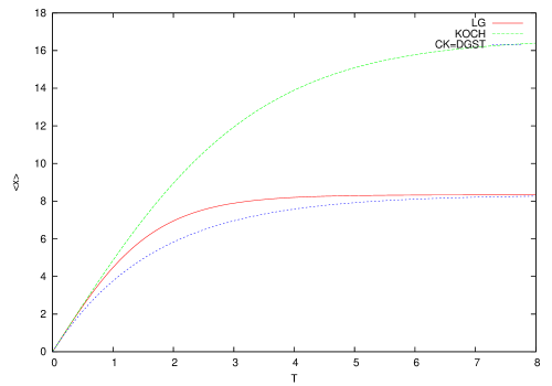
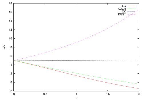
The direct calculation shows that the Wave-function still remains Gaussian. The mean value of position is
Figure 1: Comparison of the mean values of position and velocity obtained by various methods
The results obtained by Kochan’s (abbr. Koch) approachKochan2010219 are
The results obtained by Caldirola-Kanai (abbr. CK) method are
The results obtained by Das’s (abbr. DGST) method are
The comparison among these results above is illustrated in Fig. 1,
where
. The curve obtained by our method is labeled with ’LG’.
It is clear that the expectation value of velocity obtained by our method and Kochan’s method look very similar. The expectation value
of position obtained by our method is quite different from that obtained by Kochan’s method, but with time evolution, obtained by our
method approaches . The reason is
Because our averaged velocity and Kochan’s averaged velocity posses a similar advantage that they decrease with respect to
time translations, also possess similar restriction that our averaged velocity is reliable in the time interval and
Kochan’s reliable interval is . Exactly at the moment , our averaged velocity becomes zero and going over,
it would produce a negative (nonphysical) mean velocity.
V Conclusion
Kochan2009IJMPA..24.5319K have compared his results with other results obtained by the method of Caldirola-Kanai and other methods.
Because the aforementioned similarity, our approach possesses the advantage of Kochan’s approach, but the position obtained by our approach likes that obtained
by CK-method. Since both Kochan’s approach and our approach are based ultimately on the classical history, this similarity exists between the approaches.
For quantization of more complicated damping mechanical systems, one can utilize numerical method to obtain classical trajectory, then
construct approximation of the Lagrangian density.
(2)L. Herrera, L. Núñez, A. Patiño, and H. Rago, “A variational principle and the classical and
quantum mechanics of the damped harmonic oscillator,” American Journal of Physics54, 273–277 (Mar. 1986).
(3)G. López and P. López, “Velocity quantization approach of the
one-dimensional dissipative harmonic oscillator,” International Journal of Theoretical Physics 45, 734–742 (2006), ISSN 0020-7748, 10.1007/s10773-006-9064-9, http://dx.doi.org/10.1007/s10773-006-9064-9.
(12)D. Kochan, “Direct quantization of equations of motion: from
classical dynamics to transition amplitudes via strings,” ArXiv High Energy Physics - Theory e-prints(Mar. 2007).
(13)T. Luo and Y. Guo, “Infinite-Dimensional Hamiltonian Description of
Dissipative Mechanical Systems,” ArXiv e-prints(Jun. 2009), arXiv:0906.3062
[math-ph].
(15)P. J. Morrison, “Hamiltonian description of the ideal fluid,” Rev. Mod. Phys.70, 467–521 (Apr 1998).
(16)P. J. Morrison, “The maxwell-vlasov equations as a continuous
hamiltonian system..” Phys. Lett. A 80, 383–386 (Apr 1980).
(17)R. P. Feynman and A. R. Hibbs, Quantum Mechanics and Path Integrals (McGraw-Hill, 1965).
(18)Richard Phillips Feynman, A NEW APPROACH TO QUANTUM THEORY, Ph.D. thesis, Princeton University (1942).
(19)U Das, S Ghosh, P Sarkar, and B Talukdar, “Quantization of dissipative systems with friction
linear in velocity,” Physica Scripta 71, 235 (2005), http://stacks.iop.org/1402-4896/71/i=3/a=002.