Electrical detection of free induction decay and Hahn echoes in phosphorus doped silicon

Abstract

Paramagnetic centers in a solid-state environment usually give rise to inhomogenously broadened electron paramagnetic resonance (EPR) lines, making conventionally detected free induction decay (FID) signals disappear within the spectrometer dead time. Here, experimental results of an electrically detected FID of phosphorus donors in silicon epilayers with natural isotope composition are presented, showing Ramsey fringes within the first $150$ ns. An analytical model is developed to account for the data obtained as well as for the results of analogous two-pulse echo experiments. The results of a numerical calculation are further presented to assess the capability of the method to study spin-spin interactions.

I introduction

Solid-state based quantum computer (QC) architectures have recently attracted considerable interest due to the prospect of possible scalability. Several implementations have been proposed, such as superconducting tunnel junctions Makhlin et al. (2001), nuclear spins in crystal lattices Yamaguchi and Yamamoto (1999), nuclear spins of donors in Si Kane (1998), and electron spins localized in quantum dots (QDs) Loss and DiVincenzo (1998); Imamoglu et al. (1999) or at donors Vrijen et al. (2000). However, a realistic solid-state environment introduces an intrinsic inhomogeneity of the qubit properties due to impurities, defects, interfaces etc., resulting in possible computational errors. Nevertheless, fault-tolerant error correction schemes promise to compensate such errors up to a certain level DiVincenzo and Shor (1996); Knill et al. (1998); Steane (1999), making a quantification of the inhomogeneity a crucial step in the assessment of the suitability of specific physical realizations of qubits for QC.

In the case of QDs and donors, the Zeeman levels of the electron spin in an external magnetic field are used as the qubit states. The Zeeman energy of each electron spin will vary within a spin ensemble, e.g. due to the random orientation of nuclear spins in the lattice that generate a spatially fluctuating local magnetic field at the position of each electron spin. The resulting distribution $\Phi(\omega_{\mathrm{S}})$ of the Larmor frequencies $\omega_{\mathrm{S}}$ of the electron spins can be quantified in the frequency domain by the inhomogenous linewidth obtained from a traditional continuous wave (cw) electron paramagnetic resonance (EPR) experiment Abe et al. (2010a). Alternatively, a time domain analysis of $\Phi(\omega_{\mathrm{S}})$ can be carried out by measuring the decay of the transverse magnetization in the free induction decay (FID) of a conventional pulsed EPR experiment. The problem encountered in both methods is their respective detection limit which is far above the number of spins present in nanoscale structures proposed for QCs. Moreover, FID has not seen a widespread application for studies of paramagnetic species in solids since the broad Larmor frequency distribution usually encountered in solid-state spin systems makes the FID signal disappear on a time scale that is usually much shorter than the spectrometer dead time $t_{\mathrm{D}}$ after a microwave pulse of typically $100-200$ ns Schweiger and Jeschke (2001); Dikanov and Tsvetkov (1992); Blok et al. (2009).

Optically and electrically detected magnetic resonance experiments (ODMR and EDMR, respectively) have shown much promise since they exceed conventional EPR concerning detection sensitivity by at least six orders of magnitude Jelezko et al. (2004); McCamey et al. (2006). In the case of phosphorus donors (³¹P) in silicon, the development of pulsed EDMR (pEDMR) Boehme and Lips (2001, 2003); Stegner et al. (2006) has paved the way for studying dynamical properties of spin systems by applying different microwave pulse sequences, such as using the Hahn-echo sequence to study coherence times $T_{2}$ Huebl et al. (2008), or the inversion recovery sequence to study spin-lattice relaxation times $T_{1}$ Paik et al. (2010). The underlying principle of pEDMR on ³¹P donors is the use of microwave pulses for the generation of coherent states of ³¹P spins, which can be detected by transient photoconductivity measurements Boehme and Lips (2003); Stegner et al. (2006), making use of spin-dependent recombination of spin pairs formed by ³¹P and paramagnetic Si/SiO₂ interface states Kaplan et al. (1978); Hoehne et al. (2010).

In current pulsed EPR, the dead-time problem of FID has been circumvented by several techniques such as high-frequency EPR Blok et al. (2009), FID-detected hole burning Schweiger and Jeschke (2001) or detection of the EPR spectra by the Electron Spin Echo (ESE), although the latter is more sensitive to distortions through nuclear modulations in contrast to FID Schweiger and Jeschke (2001); Blok et al. (2009). In this paper, we study the possibility of electrically detecting (ED) FID using a tomography technique developed earlier Huebl et al. (2008) to investigate the Larmor frequency distribution $\Phi(\omega_{\mathrm{S}})$ of a ³¹P ensemble in natural silicon (^natSi). It is shown that information within the usual dead time of conventional EPR-detected FID can be obtained. An analytical equation is deduced to describe the experimental data, which in turn agrees well with the results of continuous wave (cw) EDMR experiments. Furthermore, a numerical study is performed to assess the EDFID technique in terms of its capability to quantitatively investigate the coupling of spin pairs.

II experimental details

The sample used in this work is fabricated by chemical vapor deposition and consists of a $22$ nm thick ^natSi layer with $\mathrm{[P]}=9\times 10^{16}$ cm^-3 covered by a native oxide. It is grown on a $2.5$ µm thick, nominally undoped ^natSi buffer on a silicon-on-insulator substrate. Evaporated interdigit Cr/Au contacts with a period of $20$ µm covering an active area of $2\times 2.25$ mm² are biased with $100$ mV, resulting in a current of $\approx 80$ µA under illumination with white light. The major paramagnetic states are identified in cwEDMR experiments performed in a Bruker X-band dielectric microwave resonator for pulsed EPR. The microwave frequency of $\nu_{\mathrm{mw}}=\omega_{\mathrm{mw}}/(2\pi)=9.7400$ GHz is provided by an HP83640 microwave synthesizer. The measurements are performed at $5.5$ K in a helium gas flow cryostat. The samples are oriented in an external magnetic field $B_{0}$ with the [001] axis of the Si wafer parallel to $B_{0}$.

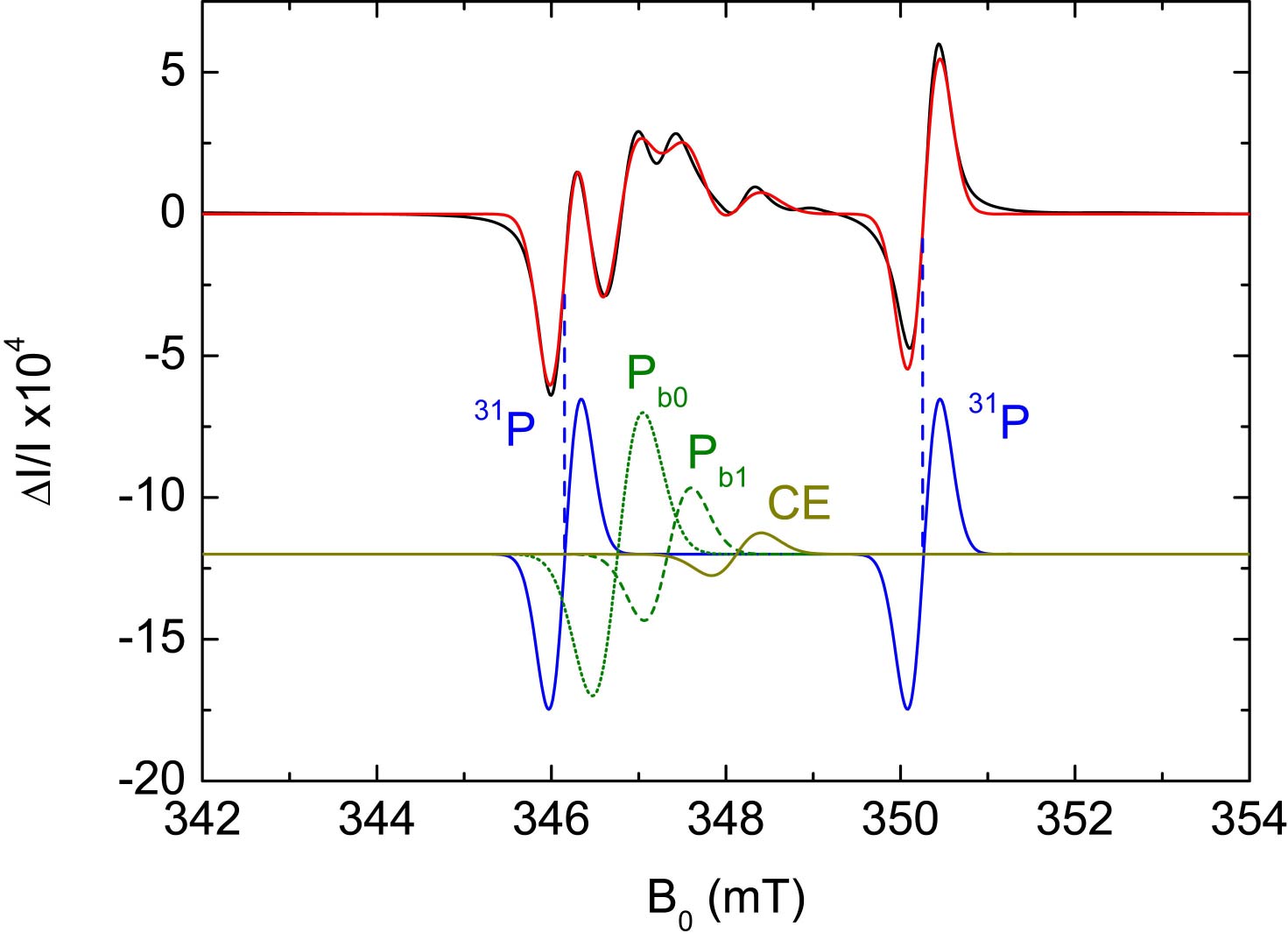
Figure 1: First derivative spectrum of the relative change $\Delta I/I$ of the photocurrent in a cwEDMR experiment on ^natSi:P with a magnetic field modulation amplitude of $0.2$ mT. The red curve represents a fit using Gaussian lineshapes and equal amplitudes of both ³¹P resonance lines. The constituent lines of the fit are shown below for better visibility.

The first derivative of the relative current change $\Delta I/I$ [cf. Fig. 1] is measured with magnetic field modulation and lock-in detection as a function of $B_{0}$ provided by a Bruker BE 25 electromagnet. We used the two pronounced ³¹P hyperfine resonance lines (denoted hf(³¹P)) at $B_{0}=346.17$ mT and $B_{0}=350.27$ mT to calibrate the magnetic field $B_{0}$ such that their center field corresponds to $g=1.9985$ Feher (1959). In addition, a resonance line at $g=2.0069\pm 0.0004$ arising from the P_b0 center at the Si/SiO₂ interface can be observed in accordance with previous studies for $B_{0}$||[001] Poindexter et al. (1981). A further resonance line is observed at $g=2.0036\pm 0.0004$ which, due to its $g$-factor, is attributed to the P_b1 center Stesmans and Afanas’ev (1998a). We are aware of the fact that there is no concensus in the literature whether the P_b1 defect is electrically active Stesmans and Afanas’ev (1998b); Mishima et al. (1999) and therefore, measurements of the angular dependence of the $g$-factor or the hyperfine interactions with ²⁹Si nuclei would be needed for an unambiguous identification. The small resonance line at $B_{0}=348.12$ mT could be attributed to conduction band electrons (CE) with a $g$-factor of $g\approx 1.9990\pm 0.0004$ Young et al. (1997). A fit assuming Gaussian line shapes and equal amplitudes of both ³¹P resonance lines is indicated by the red line in Fig. 1. The decomposition of the fitted spectrum is shown in the lower part of Fig. 1. An analysis of the isolated high-field hf(³¹P) line yields a peak-to-peak line width of $\Delta B_{\mathrm{PP}}^{\mathrm{cwEDMR}}=0.30\pm 0.03$ mT after correcting for the influence of magnetic field modulation Poole (1983). This line broadening is predominantly inhomogeneous, caused by randomly oriented nuclear spins of the ²⁹Si isotope in natural Si, which give rise to an unresolved superhyperfine multiplet Abe et al. (2010b). Homogeneous broadening only plays a minor role since $T_{1}$ and $T_{2}$ times of the ³¹P donor spins determined by ED inversion recovery Paik et al. (2010) and ED Hahn echo Huebl et al. (2008) experiments on this sample yield $T_{1}\approx 5.3$ µs and $T_{2}\approx 3.3$ µs, respectively, when the measured decays are fitted by a single exponential dependence.

The pulsed EDMR experiments are performed at a microwave frequency of $\nu_{\mathrm{mw}}=\omega_{\mathrm{mw}}/(2\pi)=9.7331$ GHz under the same orientation of the sample as the cwEDMR experiments. For all pulsed measurements, the magnetic field $B_{0}$ is corrected by the magnetic field offset determined by cwEDMR. The microwave pulses are shaped using a SPINCORE PulseBlasterESR-Pro 400 MHz pulse generator and a system of microwave mixers, and are then amplified by an Applied Systems Engineering 117X traveling wave tube with a maximum peak power of 1 kW. The actual pulse shapes coupled into the resonator are checked in reflection experiments. The quality factor of the dielectric resonator is adjusted to make a compromise between sufficient excitation bandwidth and a microwave magnetic field $B_{1}$ high enough for coherent spin manipulation. The adjustment of the microwave power is achieved by a tuneable attenuator; the $\pi/2$-pulse time of $\tau_{\pi/2}=15$ ns corresponding to $B_{1}=0.6$ mT used throughout this paper is determined in Rabi-oscillation experiments as previously developed Boehme and Lips (2003); Stegner et al. (2006). The current transients are acquired using a current amplifier followed by a voltage amplifier and a fast data aquisition card. To improve the signal-to-noise ratio, we applied a two-step phase cycling sequence where the phase of the last $\pi/2$ pulse was switched by 180^∘ at a frequency of $\approx 5$ Hz and the signals for each phase are then subtracted from each other. Switching the phases at a frequency of several Hz has the same purpose as a lock-in detection scheme and improves the signal-to-noise ratio by reducing the effects of $1/f$-noise in the measurement setup.

III results and discussion

III.1 Electrically detected FID

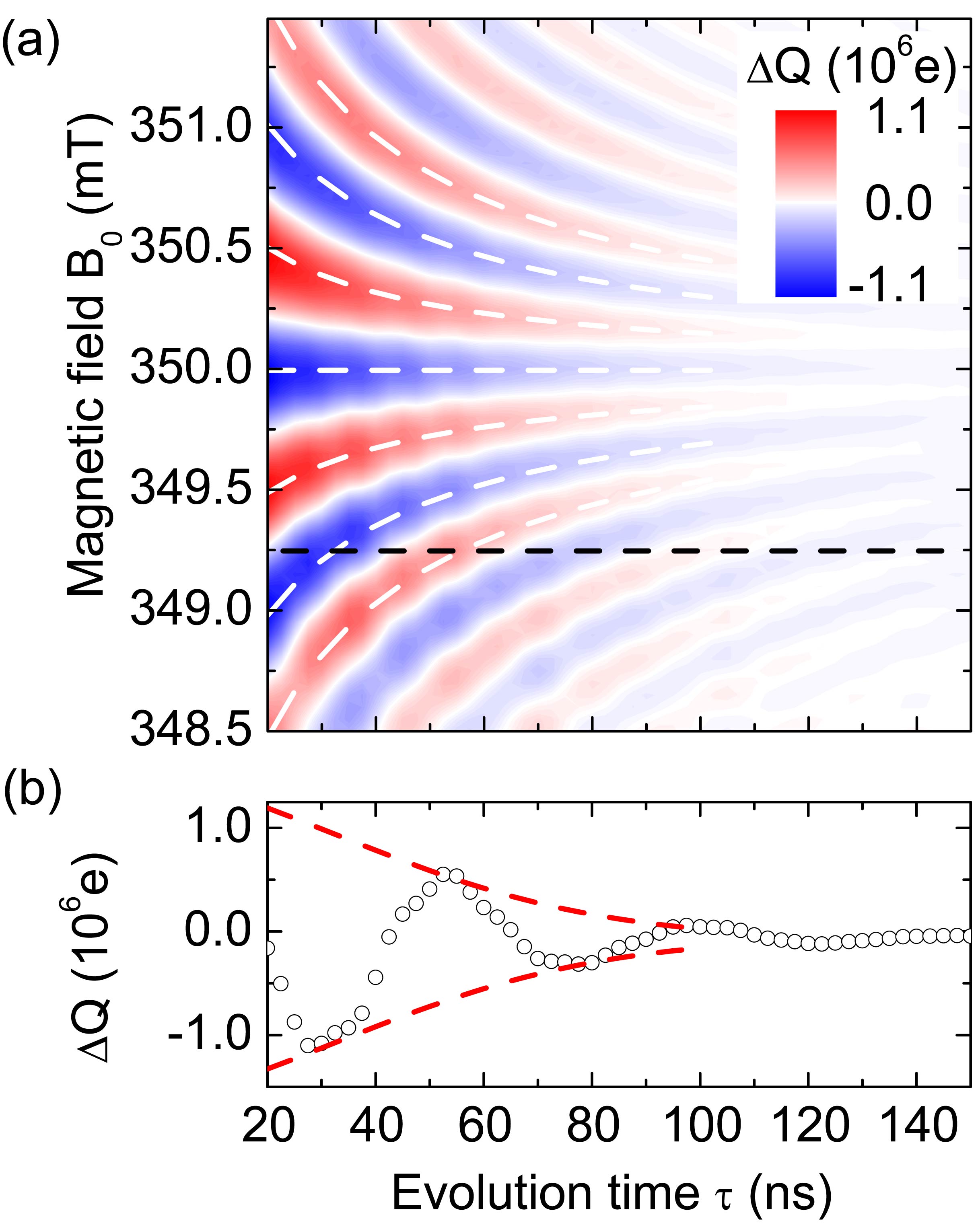
Figure 2: Electrically detected free induction decay or Ramsey experiment on the high-field hf(³¹P) resonance. (a) Contour plot of $\Delta Q$ as a function of the external magnetic field $B_{0}$ and the free evolution time $\tau$. White dashed curves mark the positions of local extrema of $\Delta Q$ described by Eq. (2). The black dashed line indicates the position where the cross-sectional chart shown in panel (b) is taken. (b) Cross-section of $\Delta Q$ along the evolution time axis at $B_{0}=349.25$ mT. Red dashed curves illustrate the Gaussian-shape damping of the oscillation amplitude.

The EDFID tomography is performed by a $\pi/2$-$\tau$-$\pi/2$ pulse sequence with varying evolution time $\tau$, consisting of the conventional free induction pulse sequence $\pi/2\mbox{-}\tau$ followed by a $\pi/2$-projection pulse as usually applied in multi-pulse EDMR experiments Huebl et al. (2008); Paik et al. (2010). Hence, it coincides with the pulse sequence of the Ramsey experiment Ramsey (1950). The photocurrent transients measured for each $B_{0}$ and $\tau$ are integrated over a fixed recording time interval satisfying the criteria described in Ref. Gliesche et al. (2008), resulting in a charge difference $\Delta Q$. Figure 2 shows experimental results of an EDFID tomography experiment on the isolated high-field hf(³¹P) line.

We will now show that the pattern in Fig. 2 (a), which is characteristic of an EDFID can be understood by a simple model in which the contribution of the state of each spin pair at the end of the second $\pi/2$ pulse is proportional to its projection onto the singlet state $|S\rangle$ Boehme and Lips (2003); Stegner et al. (2006). Hence, the measured charge $Q\propto-S^{\mathrm{av}}(\tau)=-\mathrm{Tr}(|S\rangle\langle S|\hat{\rho})$ reveals the average singlet content of the spin pair ensemble described by the density operator $\hat{\rho}$. This is in contrast to conventional ESR, where for an FID the magnetization after a $\pi/2$ pulse is detected. For microwave frequencies close to the Larmor frequency of the high-field hf(³¹P), the singlet content $S(\tau)$ of each spin pair reflects the dynamics of only this spin species Boehme and Lips (2003) while in a first approximation the spin state of P_b0 is unaltered and just serves as a projection partner. This is justified since the separation of the Larmor frequencies of the ³¹P and P_b0 spins for the high-field hf(³¹P) resonance is approximately one order of magnitude larger than the on-resonance Rabi frequency $\omega_{1}=g\mu_{\mathrm{B}}B_{1}/\hbar$. The minor effects of the off-resonance excitation of the other resonance lines can be seen as small oscillations on the Ramsey pattern in Fig. 2 (a) at magnetic fields lower than 350 mT. We also neglect spin-spin interaction and incoherent processes during the pulse sequence. The former will be addressed in Sec. III.3 and the latter is a valid assumption since the time constant for the fastest incoherent process is $T_{2}\approx 3.3$ µs as measured in ED Hahn echo decay experiments on this sample. With these assumptions, an expression for the theoretically expected signal

$$\Delta Q\propto-\exp\left[-\frac{1}{2}\frac{\sigma_{\omega}^{2}\tilde{\omega}_{1}^{2}}{\sigma_{\omega}^{2}+\tilde{\omega}_{1}^{2}}\tau^{2}\right]\cos\left[\frac{\tilde{\omega}_{1}^{2}}{\sigma_{\omega}^{2}+\tilde{\omega}_{1}^{2}}\Delta\omega\tau\right]$$ (1)

with $\tilde{\omega}_{1}=\omega_{1}/\sqrt{2}$ and $\Delta\omega=\omega_{0}-\omega_{\mathrm{mw}}$ can be derived following Ref. Jaynes (1955); Bloom (1955) as shown in Appendix A. In Eq. (1), $\sigma_{\omega}$ quantifies the width of the Larmor frequency distribution as defined in Eq. (17). The locations of the local extrema of $\Delta Q$ are given by Eq. (20) as

$$B_{0}-B_{\mathrm{res}}=\frac{n\pi\hbar\left(1+2(\sigma_{\omega}/\omega_{1})^{2}\right)}{g\mu_{\mathrm{B}}}\frac{1}{\tau},\qquad n\in\mathbb{Z},$$ (2)

representing hyperbolas in the $B_{0}$-$\tau$-plane. These hyperbolas fit the experimentally observed pattern well, as evident from the white dashed curves in Fig. 2 (a). The exponential term in Eq. (1) describes an envelope in the time domain which shows an $\exp\left[-(\tau/T_{\mathrm{FID}})^{2}\right]$-type decay behavior DeVoe and Brewer (1978) as depicted by red dashed line in Fig. 2 (b) with the time constant

$$T_{\mathrm{FID}}=\sqrt{\frac{2}{\sigma_{\omega}^{2}}+\frac{4}{\omega_{1}^{2}}}\,.$$ (3)

This implies that for short pulses, i.e. in the high microwave power limit, $T_{\mathrm{FID}}$ is inversely proportional to the width of the Larmor frequency distribution and thus $\Delta B_{\mathrm{PP}}^{\mathrm{cwEDMR}}$ of the hf(³¹P) resonance line in cwEDMR. The actual decay characteristics deviate from the $\exp\left[-(\tau/T_{\mathrm{FID}})^{2}\right]$ behavior since the lineshape is a convolution of a Gaussian and Lorentzian lineshape rather than a pure Gaussian.

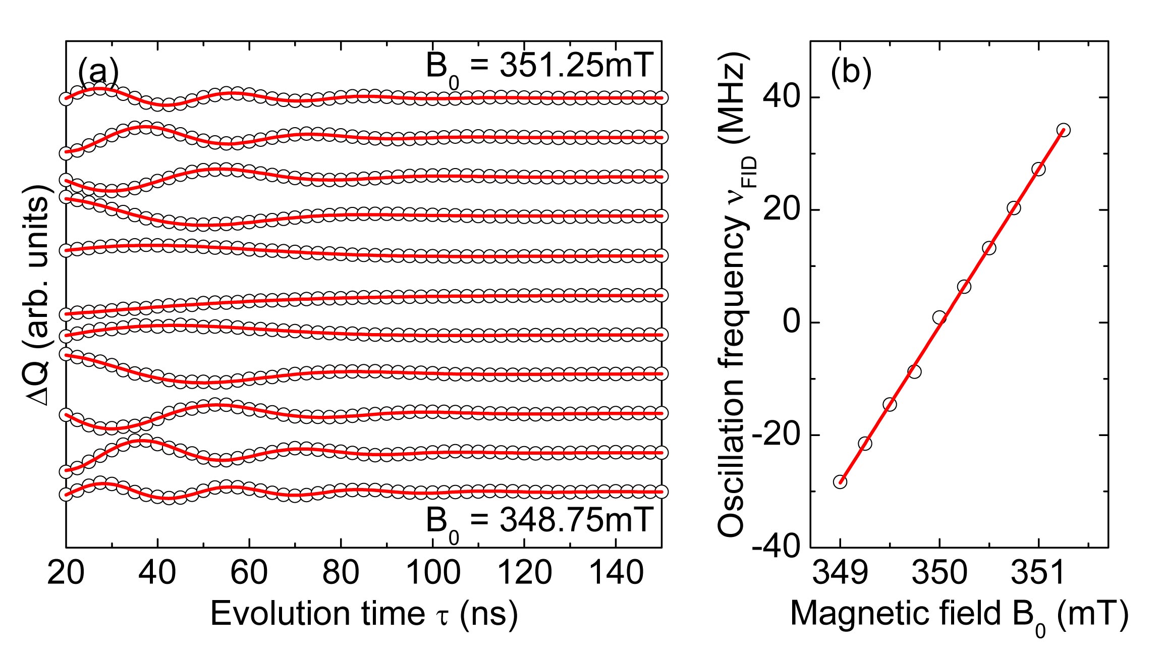
Figure 3: Oscillations in the evolution time domain. (a) Cross-sections of $\Delta Q$ along the evolution time axis taken at different values of $B_{0}$. The damping of the oscillations indicates that the spin ensemble dephases. Red curves are fits based on the model given by Eq. (4). (b) Frequency $\nu_{\mathrm{FID}}$ of the damped oscillations as a function of the external magnetic field $B_{0}$ shows a linear behavior as expected from Eq. (5).

In Fig. 3 (a), cross-sections of $\Delta Q$ along the evolution time axis taken at different values of $B_{0}$ are plotted as a function of the evolution time $\tau$, revealing strongly damped oscillations. These characteristics are consistent with those described by Eq. (1). A clear dependence of the frequencies of the damped oscillations $\nu_{\mathrm{FID}}$ on the external magnetic field $B_{0}$ can be observed. The red lines in Fig. 3(a) show fits of the oscillations by the function

$$\Delta Q\sim-Ae^{-\left(\frac{\tau+\tau_{0}}{T_{\mathrm{FID}}}\right)^{2}}\cos\left[2\pi\nu_{\mathrm{FID}}(\tau+\tau_{0})\right]$$ (4)

which is based on the model given in Eq. (1). In all the fits shown in Fig. 3 (a), a global phase correction of $\tau_{0}\approx 20$ ns has to be taken into account which is comparable to the overall pulse length of 30 ns. It can be attributed to the fact that dephasing during the pulse times can not be neglected due to the finite pulse width compared to the evolution time $\tau$. The values of $\nu_{\mathrm{FID}}$ obtained from the fits are plotted as a function of the external magnetic field $B_{0}$ and displayed in Fig. 3 (b). A clear linear dependence of $\nu_{\mathrm{FID}}$ on the magnetic field $B_{0}$ can be observed as expected from Eq. (1),

$$\nu_{\mathrm{FID}}=\frac{1}{2\pi}\frac{\tilde{\omega}_{1}^{2}}{\sigma_{\omega}^{2}+\tilde{\omega}_{1}^{2}}\left(\omega_{0}-\omega_{\mathrm{mw}}\right)=k\left(B_{0}-B_{\mathrm{res}}\right),$$ (5)

with $k=g\mu_{\mathrm{B}}/[h(1+2(\sigma_{\omega}/\omega_{1})^{2})]$. This is consistent with the linear dependence of the oscillation frequency on the detuning in a Ramsey experiment Plourde et al. (2005); Wallraff et al. (2005). From a linear fit of the data the value of $B_{\mathrm{res}}=350.02\pm 0.01$ mT is obtained, which corresponds to the center position of the high-field hf(³¹P) resonance line. Using Eq. (3) and $2\pi/\omega_{1}=60$ ns, the average value $T_{\mathrm{FID}}=64.4\pm 5$ ns obtained from the fits of the damped oscillations can be related to an expected cwEDMR peak-to-peak line width of $\Delta B_{\mathrm{PP}}^{\mathrm{FID}}=2\hbar\sigma_{\omega}/(g\mu_{\mathrm{B}})=0.26\pm 0.02\mbox{ mT}$. This is in agreement with the result obtained from cwEDMR $\Delta B_{\mathrm{PP}}^{\mathrm{cwEDMR}}=0.30\pm 0.03\mbox{ mT}$, demonstrating the consistency of the experiments.

III.2 Electrically detected Hahn echo.jpg

Electrically detected echo sequences have been previously used to study $T_{2}$ Huebl et al. (2008) and $T_{1}$ times Paik et al. (2010) of phosphorus donors near Si/SiO₂ interface defects. In this section, we will present detailed experimental results of the electrically detected Hahn echo measurement with a focus on the fine structure of the echo response.

The echo is measured using the previously developed tomography technique Huebl et al. (2008) extending the pulse sequence $\pi/2$-$\tau_{1}$-$\pi$-$\tau_{2}$ of the conventional two-pulse spin echo containing two free evolution times $\tau_{1}$ and $\tau_{2}$ by a final $\pi/2$ pulse as applied in the EDFID technique. The measurements are conducted under the same experimental conditions as the EDFID experiments.

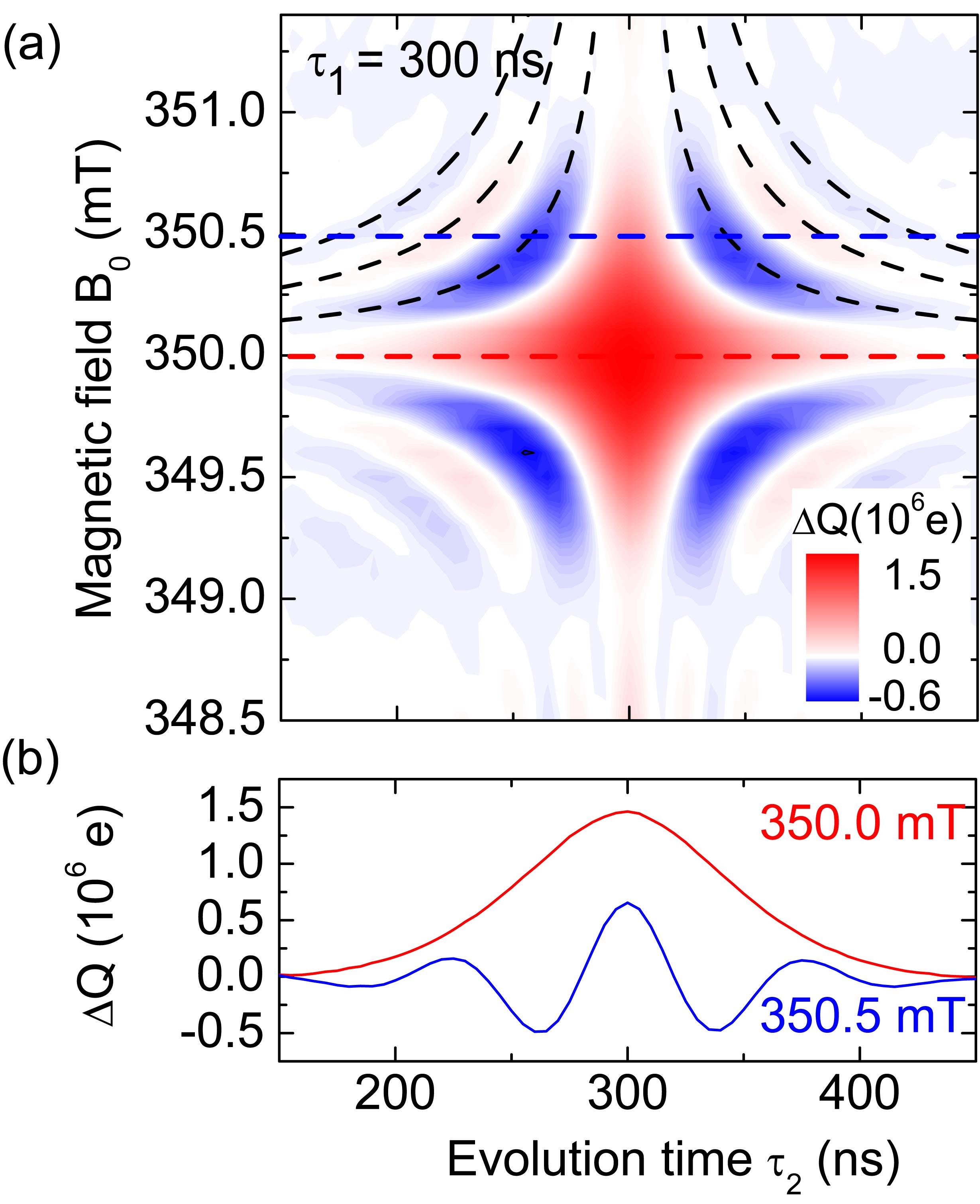
Figure 4: Electrically detected two-pulse Hahn echo on the high-field hf(³¹P) resonance with $\tau_{1}=300$ ns. (a) Contour plot of $\Delta Q$ as a function of the external magnetic field $B_{0}$ and the free evolution time $\tau_{2}$. Black dashed lines mark the hyperbola pattern according to Eq. (6). Red and blue dashed lines indicate positions where cross-sectional diagrams shown in panel (b) are taken. (b) Cross-section of $\Delta Q$ along the evolution time axis at resonance condition (red line, $B_{0}=350.0$ mT) and for the off resonant case (blue line, $B_{0}=350.5$ mT). Please refer to the text for details.

Figure 4 shows experimental results of an ED spin echo tomography experiment on the isolated high-field hf(³¹P) line with $\tau_{1}=300$ ns held fix. The values of $\Delta Q$ plotted as a function of $B_{0}$ and $\tau_{2}$ [Fig. 4(a)] are obtained in the same way as described in the EDFID section. Cross-sections along the evolution time axis are displayed in Fig. 4(b). The red curve taken at the resonance field $B_{0}=350.0$ mT shows a Gaussian-shaped peak centered around $\tau_{2}=\tau_{1}=300$ ns. The cross section of $\Delta Q$ at the off-resonance field $B_{0}=350.5$ mT, which is represented by the blue curve, shows oscillations as a function of the evolution time $\tau_{2}$ with a maximum at $\tau_{2}=\tau_{1}=300$ ns, which decay for $|\tau_{2}-\tau_{1}|\gg 100$ ns.

The characteristic pattern indicated by the black dashed hyperbolas can be understood by the same quantitative model described in the previous section on EDFID. The singlet content $S(\tau)$ proportional to the recombination probability $P_{\uparrow,\downarrow}$ of a single spin after a $\pi/2$-$\tau_{1}$-$\pi$-$\tau_{2}$-$\pi/2$ pulse sequence can be calculated using the matrix formalism described in Ref. Jaynes (1955); Bloom (1955). For a Larmor frequency distribution modelled by a Gaussian with standard deviation $\sigma_{\omega}$ centered about $\omega_{0}$, we can derive analogously to Eq. (19) that

$$\Delta Q \propto \exp\left[-\frac{1}{2}\frac{\sigma_{\omega}^{2}\bar{\omega}_{1}^{2}}{\sigma_{\omega}^{2}+\bar{\omega}_{1}^{2}}(\tau_{2}-\tau_{1})^{2}\right]$$ (6)

$$\times\cos\left[\frac{\bar{\omega}_{1}^{2}}{\sigma_{\omega}^{2}+\bar{\omega}_{1}^{2}}(\omega_{0}-\omega_{\mathrm{mw}})(\tau_{2}-\tau_{1})\right]$$

with $\bar{\omega}_{1}=\omega_{1}/2$  fac .

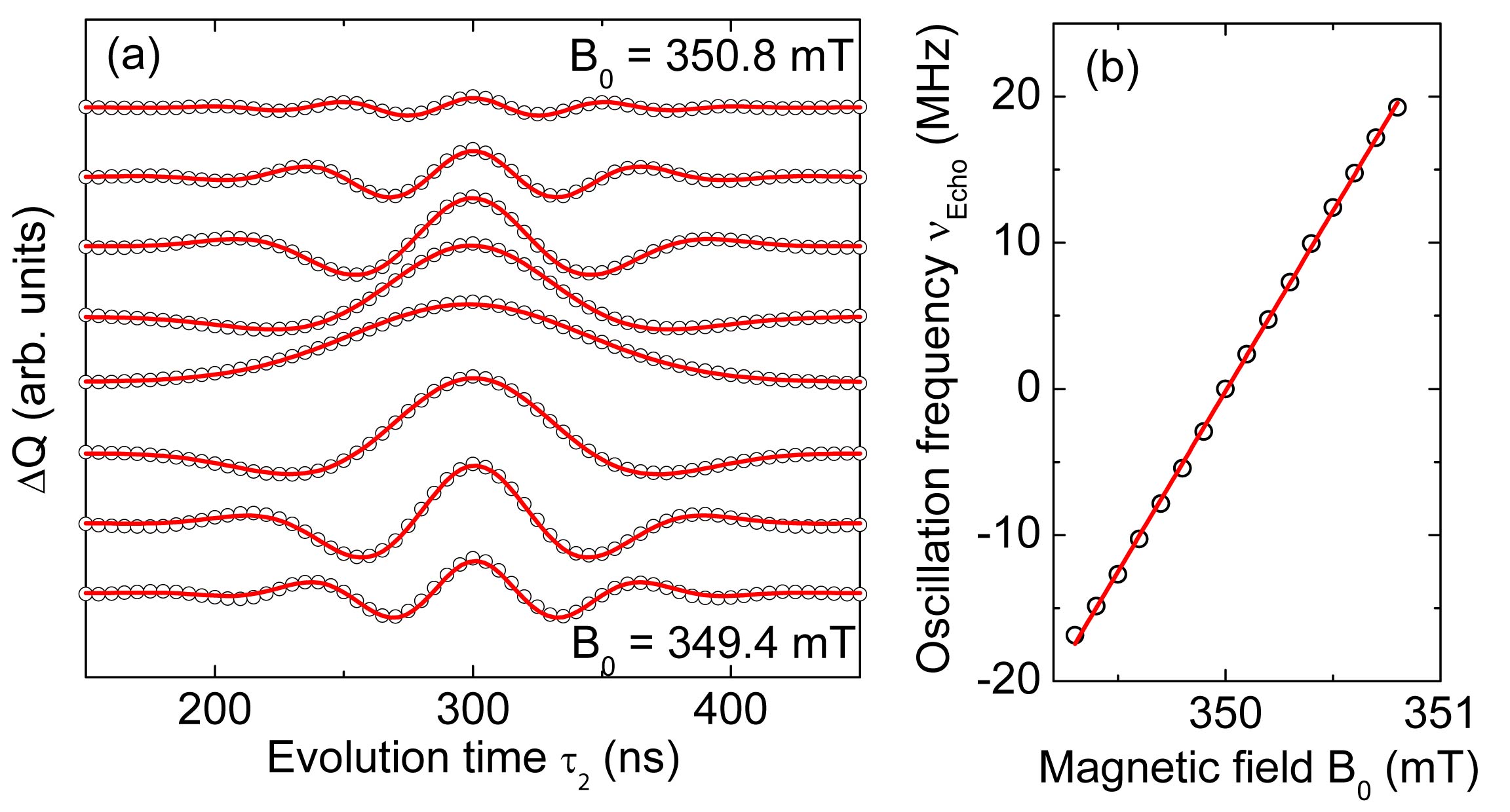
Figure 5: Oscillations in the evolution time domain. (a) Cross-sections of $\Delta Q$ along the evolution time axis taken at different values of $B_{0}$. Red curves are fits based on the model given by Eq. (6). (b) The frequency $\nu_{\mathrm{Echo}}$ of the damped oscillations as a function of the external magnetic field $B_{0}$ shows a linear behavior as expected from Eq. (7).

Similar to the analysis of the EDFID experiment, various cross-sections of $\Delta Q$ along the evolution time axis are taken and shown in Fig. 5(a). Data fitting based on Eq. (6) is performed and illustrated by the red curves. The oscillation frequency $\nu_{\mathrm{Echo}}$ obtained from the fits is plotted as a function of the external magnetic field $B_{0}$ [Fig. 5(b)], where a linear dependence of $\nu_{\mathrm{Echo}}$ as a function of $B_{0}$ can be observed as expected from

$$\nu_{\mathrm{Echo}}=\frac{1}{2\pi}\frac{\bar{\omega}_{1}^{2}}{\sigma_{\omega}^{2}+\bar{\omega}_{1}^{2}}\left(\omega_{0}-\omega_{\mathrm{mw}}\right)=k^{\prime}\left(B_{0}-B_{\mathrm{res}}\right),$$ (7)

with $k^{\prime}=g\mu_{\mathrm{B}}/[h(1+4(\sigma_{\omega}/\omega_{1})^{2})]$ analogous to Eq. (5). The exponential term in Eq. (6) describes a Gaussian envelope in the time domain with full width at half maximum (FWHM)

$$W_{\mathrm{echo}}=2\sqrt{2\ln 2}\sqrt{\frac{1}{\sigma_{\omega}^{2}}+\frac{4}{\omega_{1}^{2}}}\,.$$ (8)

From the fits of the data, an average value of $W_{\mathrm{echo}}=106.9\pm 4$ ns is obtained, corresponding to an expected cwEDMR linewidth of $\Delta B_{\mathrm{PP}}^{\mathrm{Echo}}=0.28\pm 0.01$ mT. This value is consistent with the values $\Delta B_{\mathrm{PP}}^{\mathrm{cwEDMR}}=0.30\pm 0.03$ mT and $\Delta B_{\mathrm{PP}}^{\mathrm{FID}}=0.26\pm 0.02$ mT obtained from previous experiments within the accuracy limits. Therefore, the ED Hahn echo response on the high-field hf(³¹P) resonance shows the same fine structure as the EDFID experiment and can be explained by the same model as expected from the fact that the echo pulse sequence consists of two FIDs back to back Weil and Bolton (2007). However, the small oscillations seen in EDFID are not observed in the ED Hahn echo response, since they are fully defocussed due to the additional central $\pi$-pulse.

III.3 Spin-spin coupling

So far the experimental results have been discussed in the context of off-resonance oscillations and dephasing due to inhomogeneous line broadening. In different previous studies Fukui et al. (2000); Gliesche et al. (2008), the possible impact of coupling between the partners of the spin pair on EDMR experiments has been discussed. In the following, results of a numerical study of the EDFID experiment discussed above are presented, focussing on the possibility of EDFID to estimate the coupling strength.

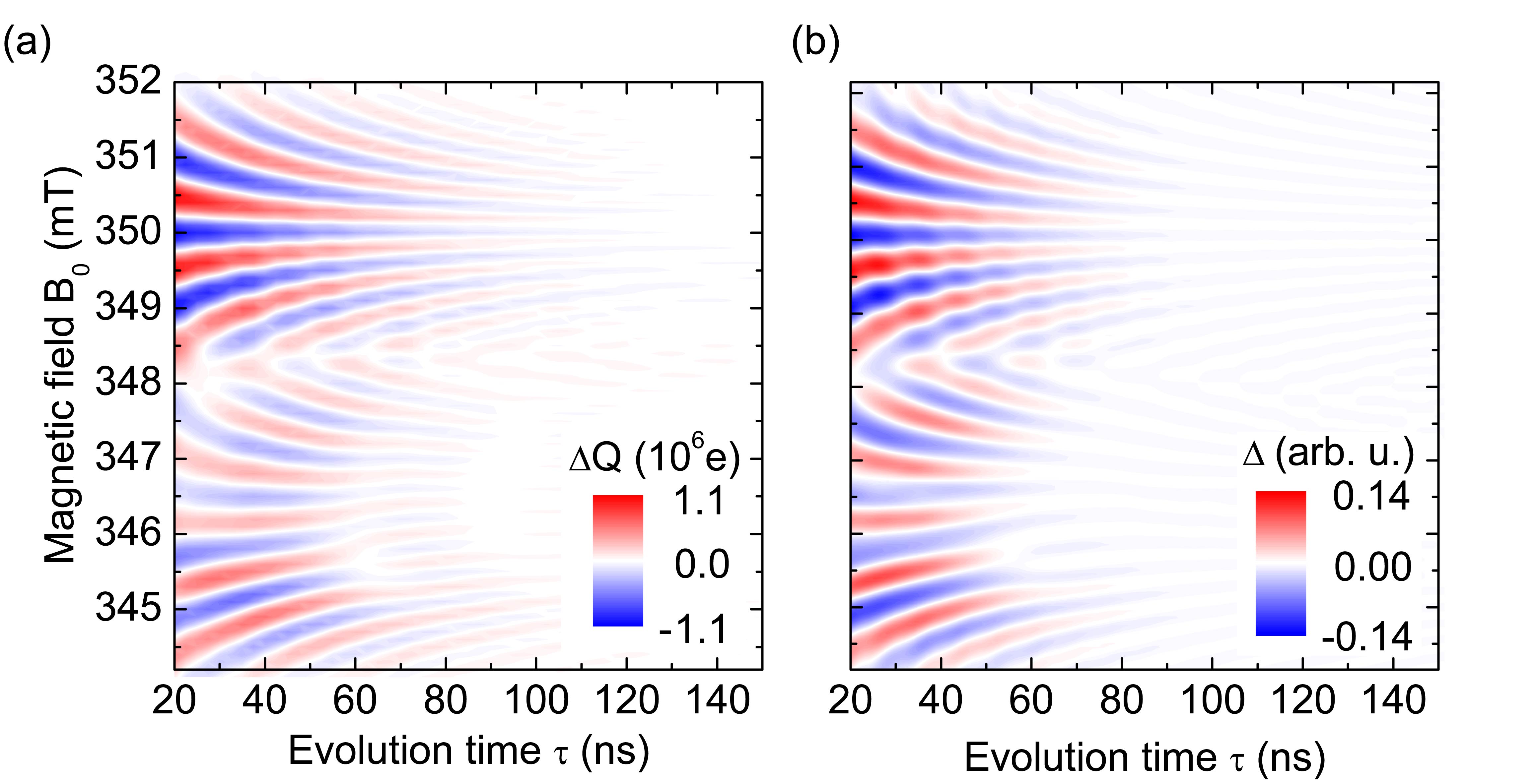
Figure 6: (a) Experimental results of the EDFID measurement showing all spectral features. (b) Simulation for $J\leavevmode\nobreak\ =\leavevmode\nobreak\ 0$ MHz. In both simulation and experimental results, the characteristic Ramsey pattern can be clearly seen at the position of the high-field hf(³¹P) resonance, whereas the patterns at the low-field hf(³¹P) and the P_b0 resonances are more complicated due to mutual interference.

The system is modelled by an ensemble of spin $S=1/2$ pairs described by the density operator $\hat{\rho}$. The Hamiltonian of an individual pair is defined as

$$\hat{\mathcal{H}}=\hat{\mathcal{H}}_{0}+\hat{\mathcal{H}}_{\mathrm{J}}+\hat{\mathcal{H}}_{1}(t)$$ (9)

with

$$\hat{\mathcal{H}}_{0} = \frac{1}{2}g_{\mathrm{P}}\mu_{\mathrm{B}}\left(B_{0}\pm B_{\mathrm{HF}}/2+B_{\mathrm{SHF}}\right)\hat{\sigma}_{z}^{\mathrm{P}}$$ (10)

$$+\frac{1}{2}g_{\mathrm{db}}\mu_{\mathrm{B}}\left(B_{0}+B_{\mathrm{\Delta db}}\right)\hat{\sigma}_{z}^{\mathrm{db}}$$

representing the static uncoupled Hamiltonian in the presence of a constant magnetic field $\mathbf{B}_{0}=B_{0}\mathbf{e}_{z}$ superimposed with the hyperfine field of ³¹P $B_{\mathrm{HF}}=4.2$ mT and the superhyperfine field $B_{\mathrm{SHF}}$ at the position of the donor, where the latter can be considered fixed for timescales shorter than the precession period of ²⁹Si nucleus Lee et al. (2005). $B_{\mathrm{\Delta db}}$ is the local shift of the static magnetic field at the position of the P_b0 center due to effects such as disorder and superhyperfine interactions. The $\hat{\sigma}_{x,y,z}$ denote the Pauli spin operators. The circularly polarized microwave of angular frequency $\omega_{\mathrm{mw}}$ and magnitude $B_{1}$ is represented in the rotating frame by

$$\hat{\mathcal{H}}_{1}=\mu_{\mathrm{B}}B_{1}\left(g_{\mathrm{P}}\hat{\sigma}_{x}^{\mathrm{P}}+g_{\mathrm{db}}\hat{\sigma}_{x}^{\mathrm{db}}\right),$$ (11)

which is nonzero during the pulse. Spin-spin interaction is modelled by an exchange coupling Hamiltonian represented by

$$\hat{\mathcal{H}}_{\mathrm{J}}=\hbar J\hat{\boldsymbol{\sigma}}^{\mathrm{P}}\cdot\hat{\boldsymbol{\sigma}}^{\mathrm{db}}/4,$$ (12)

with $\hat{\boldsymbol{\sigma}}=(\hat{\sigma}_{x},\hat{\sigma}_{y},\hat{\sigma}_{z})^{T}$. The dipolar coupling is smaller than 1 MHz for interspin distances larger than 3 nm, which is neglected here for simplicity. The simulation of the spin pair ensemble dynamics is based on the Liouville equation $\partial_{t}\hat{\rho}=i[\hat{\rho},\hat{\mathcal{H}}]^{-}/\hbar$ in which, in contrast to Eq. (5) of Ref. Boehme and Lips (2003), all terms related to incoherent processes are dropped since the time constant of the fastest incoherent process is more than one order of magnitude larger than the duration of the pulse sequence, as already mentioned in Section II. The initial steady state of the density operator is assumed to be given by the pure triplet state $\hat{\rho}^{\mathrm{S}}=\left(|T_{+}\rangle\langle T_{+}|+|T_{-}\rangle\langle T_{-}|\right)/2$ with $|T_{+}\rangle=|\!\!\uparrow^{\mathrm{db}}\uparrow^{\mathrm{P}}\rangle$ and $|T_{-}\rangle=|\!\!\downarrow^{\mathrm{db}}\!\downarrow^{\mathrm{P}}\rangle$ Boehme and Lips (2003). For triplet recombination rates $r_{\mathrm{T}}$ much smaller than the singlet recombination rate $r_{\mathrm{S}}$, the observable $Q(\tau)$ reflecting the state of the pair ensemble at the end of the second $\pi/2$ pulse assumes the form $Q(\tau)\propto-\delta(\tau)=-(\delta\rho_{\uparrow^{\mathrm{db}}\downarrow^{\mathrm{P}}}+\delta\rho_{\downarrow^{\mathrm{db}}\uparrow^{\mathrm{P}}})$ Gliesche et al. (2008), where $-\delta\rho_{ii}=-(\rho_{ii}(\tau)-\rho_{ii}^{\mathrm{S}})$ denotes the negative difference between the diagonal elements of the density matrix at the end of the second $\pi/2$-pulse and the initial steady state. The negative sign expresses the quenching of the photocurrent due to recombination. Inhomogeneous line broadening is taken into account by calculating $-\delta(\tau)$ for a single spin pair and subsequent averaging over Gaussian distributions for both $B_{\mathrm{SHF}}$ and $B_{\Delta\mathrm{db}}$ with experimentally obtained standard deviations from the pulsed EDFID spectrum shown in Fig. 6. Furthermore, the simulation takes all four combinations of spin pair formation into account, which arise from the two resonance positions of ³¹P, the P_b0, and the P_b1.

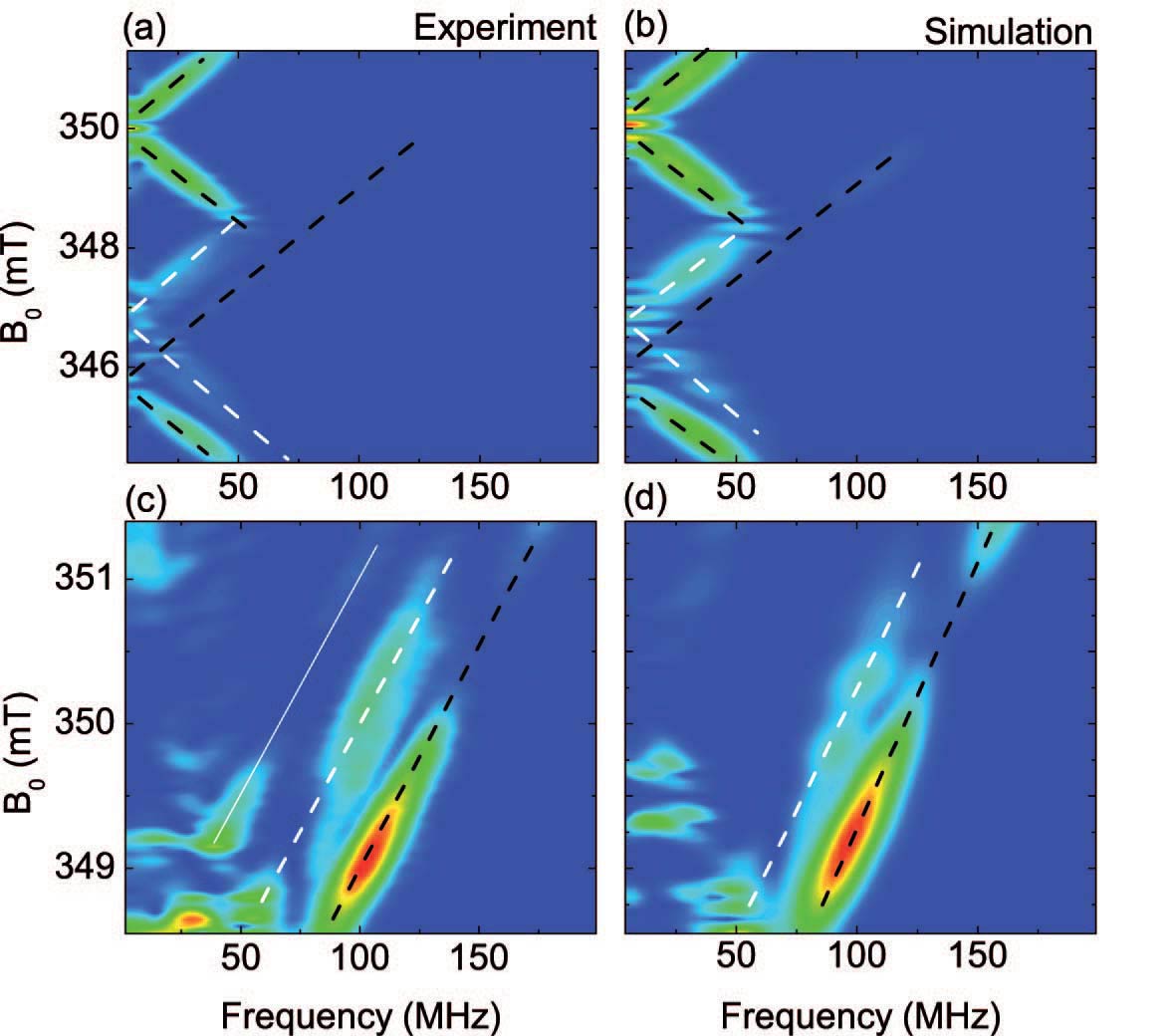
Figure 7: (a) and (b) Fourier transformation of the EDFID tomography experiment and simulation shown in Fig. 6. The linear dependence of the oscillation frequency on $B_{0}-B_{\mathrm{res}}$ described by Eq. (5) is clearly seen in the frequency domain. The two ³¹P resonances and the broader P_b0 resonance are marked by black and white dashed lines, respectively. (c) and (d) For better visibility, details of the FFT-spectrum near the high-field hf(³¹P) resonance are shown after subtracting a background of the form of Eq. (4) from the experimental and simulated data. Again, the low-field hf(³¹P) resonance and the P_b0 resonance are marked by black and white dashed lines. An additional resonance, indicated by the solid white line, can be seen in the experimental data. Its spectral position is in accordance with the small central line observed in cwEDMR (see Fig. 1).

Figure 6(a) shows the complete experimental results encompassing all resonances of the EDFID tomography experiment discussed in Fig. 2(a). Figure 6(b) shows the simulation of $-\delta$ for $J=0$ as a function of $B_{0}$ and $\tau$ after subtraction of a constant background obtained from the value of $-\delta$ for large $\tau$, resulting in the quantity $\Delta$ which can be compared to $\Delta Q$ in the experiment. The characteristic patterns of simulation and experiment fit quite well. At the high-field ³¹P resonance, small oscillations superimposed on the Ramsey oscillation pattern can be seen in the experimental data as well as in the simulation. These small oscillations are due to the partial excitation of the low-field ³¹P and the P_b0 spins by the microwave pulses on the high-field ³¹P resonance. Details of these patterns are shown in the Fourier transformed data shown in Fig. 7 (a) and (b). The linear dependence of the oscillation frequency on $B_{0}-B_{\mathrm{res}}$ described by Eq. (5) is clearly visible in the frequency domain. The two ³¹P resonances and the P_b0 resonance are marked by black and white dashed lines, respectively. The P_b1 resonance is not resolved due to the spectral overlap with the P_b0 and its smaller amplitude. For better visibility, details of the FFT-spectrum near the high-field hf(³¹P) resonance are shown in panels (c) and (d) after subtracting a background of the form of Eq. (4) from the experimental and simulated data. Again, the low-field hf(³¹P) resonance and the P_b0 resonance are marked by black and white dashed lines. An additional resonance, indicated by the solid white line, can be seen in the experimental data. Its spectral position is in accordance with the small central line observed in cwEDMR (see Fig. 1). This line is not taken into account in the simulation. The intensity of the Fourier amplitude of the lines as a function of the magnetic field can be described by an equation of the form $\sin^{2}\left(\frac{\pi}{4}\sqrt{1+x^{2}}\right/(1+x^{2}))$, analogous to Eq. (13). In particular, the minima at frequencies of $\approx 65$ MHz and $\approx 130$ MHz correspond to rotations of the spins by integer multiples of $2\pi$.

The simulation is further extended to nonzero coupling parameters with the focus on the clearly observable pattern structure on the high-field hf(³¹P) resonance, which is shown in Fig. 8.

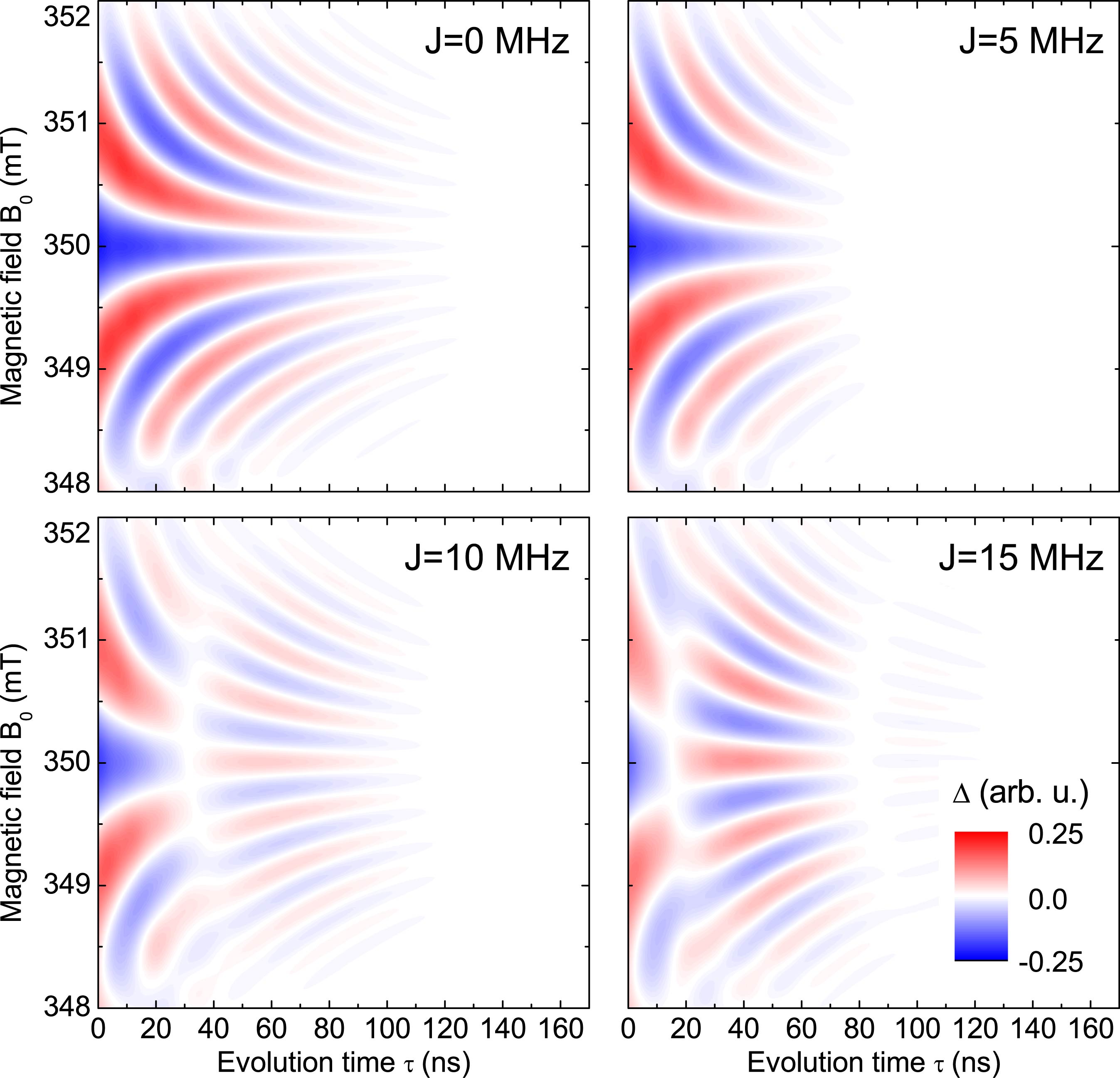
Figure 8: Simulation of the EDFID experiment at the high-field hf(³¹P) resonance for different exchange coupling parameter. An oscillation of the signal in the time-domain with the coupling frequency is expected. This oscillation is masked by the exponential decay of the signal due to dephasing and therefore can only be resolved for $J\leavevmode\nobreak\ >\leavevmode\nobreak\ 5\leavevmode\nobreak\$MHz.

Starting from $J=0$, the exchange coupling parameter is increased in steps of $5$ MHz resulting in a change of the qualitative behavior of the characteristic pattern. Whereas for $J=0$ each hyperbola (cf. Fig. 2) either indicates positions of local maxima or minima, the values of $\Delta$ on each hyperbola oscillate as a function of $\tau$ for $J\neq 0$. This behavior can be clearly observed on the axis of symmetry at $B_{0}=B_{\mathrm{res}}$, which is displayed in Fig. 9(a) for different values of $J$.

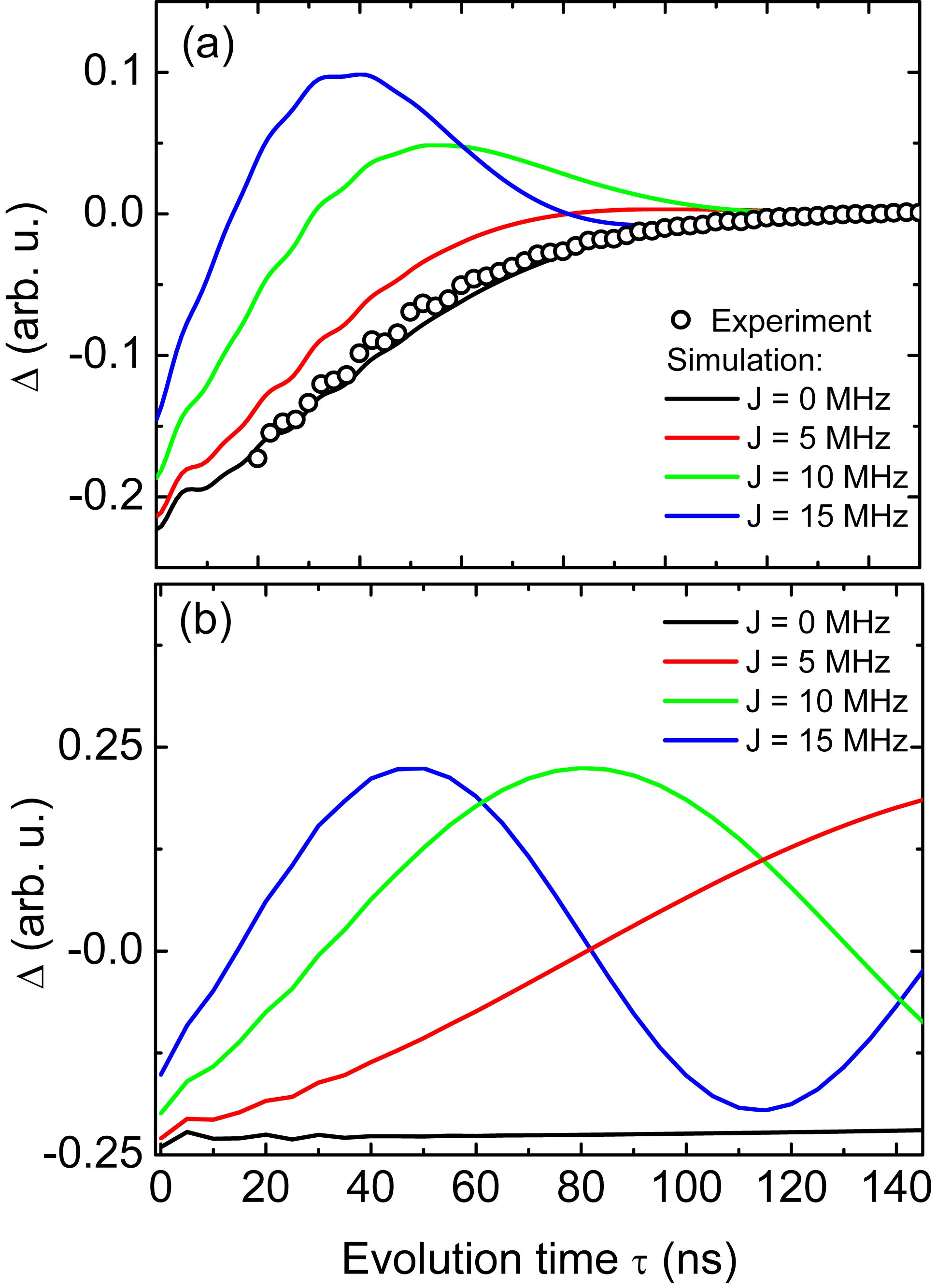
Figure 9: (a) Cross section along the $\tau$ axis at the high-field resonance field of ³¹P of the experimental data (open circles) and the simulated data (solid lines) for different exchange coupling parameter between ³¹P and P_b0. (b) Simulated data like in (a) for an isotopically purified ²⁸Si sample. Here, more oscillations caused by the weak coupling can be seen due to the longer dephasing time.

For vanishing coupling, $\Delta$ relaxes exponentially to the equilibrium. For larger values of $J$, damped oscillations of $\Delta$ with frequency $J$ are formed decaying to the equilibrium within the dephasing time $T_{\mathrm{FID}}$. Compared with the existing experimental data [cf. Fig. 3 (a)], the coupling is estimated $\ll 5$ MHz. Please note, that in these simulations only the high-field ³¹P and the P_b0 are taken into account. Therefore, the small oscillations in Fig. 9 are due to off-resonance excitations of the P_b0 spins.

Clearer insight might be obtained in an experiment using isotopically purified ²⁸Si samples as shown in the simulation in Fig. 9(b) where the line broadening (although determined by a homogeneous line width) is qualitatively modelled by a Gaussian distribution with FWHM line width of $0.023$ mT corresponding to a concentration of ²⁹Si nuclei of $\approx$ % Abe et al. (2010b). Since $T_{\mathrm{FID}}\sim 1/\sigma_{\omega}$ [cf. Eq. (3)] oscillations on the axis of symmetry could be observed within the dephasing time also for weak $J$. Qualitatively, the frequency of the oscillations increases with increasing $J$ as evident from Fig. 9(b). In the general case, distributions of exchange interaction as well as dipolar interaction have to be taken into account Boehme and Lips (2003), which would result in an averaging out of the oscillation pattern. However, previous studies have revealed that only spin-pairs within a narrow range of intra-pair distances contribute to the observed signals Paik et al. (2010), which should make an estimate of $J$ of contributing spin pairs still possible.

IV Summary

To summarize, we have used pulsed EDMR to study the free induction decay of phosphorus donor spins in silicon. We can resolve oscillations up to 150 ns limited by dephasing due to superhyperfine interactions with surrounding ²⁹Si nuclei. An analytical model is used to describe the FID of an inhomogeneously broadened line which is in good agreement with the experimental data. In addition, structures on two-pulse electron spin echoes have been measured which can be described by the same analytical model. The results of a numerical calculation are further presented and compared with the experimental data to assess the capability of the method to study spin-spin interactions. From these results, we can give an upper bound for the coupling parameter of $J\leavevmode\nobreak\ \approx\leavevmode\nobreak\ 5$ MHz in the samples studied.

Appendix A analytical expression describing the edfid pattern

In this section, Eq. (2) used to describe the pattern in Fig. 2(a) is derived. Neglecting spin-spin interactions and incoherent processes, the singlet content $S(\tau)$ is proportional to the flipping probability $P_{\uparrow,\downarrow}$ of a single spin after a $\pi/2$-$\tau$-$\pi/2$ pulse sequence, which has been investigated in studies related to nuclear magnetic resonance Jaynes (1955); Bloom (1955)

$$P_{\uparrow,\downarrow}(\tau) = 4\sin^{2}\theta\sin^{2}\left(\frac{at_{\mathrm{p}}}{2}\right)\times\left[\cos\left(\frac{\lambda\tau}{2}\right)\cos\left(\frac{at_{\mathrm{p}}}{2}\right)\right.$$ (13)

$$\left.-\cos\theta\sin\left(\frac{\lambda\tau}{2}\right)\sin\left(\frac{at_{\mathrm{p}}}{2}\right)\right]^{2}$$

with

$$\lambda=\omega_{\mathrm{S}}-\omega_{\mathrm{mw}},\quad a=\sqrt{\lambda^{2}+\omega_{1}^{2}},\quad\sin\theta=\frac{\omega_{1}}{a},$$

where $\omega_{\mathrm{S}}$ is the Larmor frequency of the ³¹P donor electron and $\omega_{\mathrm{mw}}$ the microwave frequency. $t_{\mathrm{p}}=\pi/(2\omega_{1})$ and $\tau$ denote the length of the $\pi/2$ pulse and the free evolution time, respectively. For inhomogenously broadened lines, the observable $S^{\mathrm{av}}(\tau)$ is obtained by averaging $S(\tau)\propto P_{\uparrow,\downarrow}(\tau)$ over the Larmor frequency distribution Boehme and Lips (2003)

$$S^{\mathrm{av}}(\tau)\propto\int\limits_{-\infty}^{\infty}\Phi(\omega_{\mathrm{S}})P_{\uparrow,\downarrow}(\tau,\omega_{\mathrm{S}})\mathrm{d}\omega_{\mathrm{S}}.$$ (14)

For distributions $\Phi(\omega_{\mathrm{S}})$ with a maximum at the center frequency $\omega_{0}$, the dominant term of $S^{\mathrm{av}}(\tau)$ for $\omega_{\mathrm{mw}}$ close to $\omega_{0}$ is given by

$$S^{\mathrm{av}}(\tau)\propto\int\limits_{-\infty}^{\infty}\Phi(\omega_{\mathrm{S}})\frac{\sin^{2}\left(\frac{\pi}{2}\sqrt{1+x^{2}}\right)}{1+x^{2}}\frac{1+\cos\left(\lambda\tau\right)}{2}\mathrm{d}\omega_{\mathrm{S}},$$ (15)

with $x=\lambda/\omega_{1}$, neglecting a term of $\mathcal{O}(|\omega_{\mathrm{mw}}-\omega_{S}|^{2})$. To obtain an analytical expression, Eq. (15) can be further simplified by the approximation

$$\frac{\sin^{2}\left(\frac{\pi}{2}\sqrt{1+x^{2}}\right)}{1+x^{2}}\approx\exp(-x^{2})$$ (16)

since both functions share the same leading orders in the Taylor expansion, tolerating a deviation of 6% in the integrated area within the interval defined by the zero-crossings of $\sin^{2}(...)/(1+x^{2})$ in Eq. (15). Modelling the Larmor frequency distribution by a Gaussian

$$\Phi(\omega_{\mathrm{S}})=\frac{1}{\sqrt{2\pi}\sigma_{\omega}}\exp\left[-\frac{1}{2}\left(\frac{\omega_{\mathrm{S}}-\omega_{0}}{\sigma_{\omega}}\right)^{2}\right]$$ (17)

with standard deviation $\sigma_{\omega}$ and center $\omega_{0}$, the average singlet content is given by

$$S^{\mathrm{av}} \propto \exp\left[-\frac{1}{2}\frac{\Delta\omega^{2}}{\sigma_{\omega}^{2}+\tilde{\omega}_{1}^{2}}\right]\left\{1+\exp\left[-\frac{1}{2}\frac{\sigma_{\omega}^{2}\tilde{\omega}_{1}^{2}}{\sigma_{\omega}^{2}+\tilde{\omega}_{1}^{2}}\tau^{2}\right]\right.$$ (18)

$$\left.\times\cos\left[\frac{\tilde{\omega}_{1}^{2}}{\sigma_{\omega}^{2}+\tilde{\omega}_{1}^{2}}\Delta\omega\tau\right]\right\}$$

with $\tilde{\omega}_{1}=\omega_{1}/\sqrt{2}$ and $\Delta\omega=\omega_{0}-\omega_{\mathrm{mw}}$. Since $Q\propto-S^{\mathrm{av}}$, $\Delta Q$ is proportional to $-\left[S^{\mathrm{av}}(\tau)-S^{\mathrm{av}}(\tau\to\infty)\right]$ as the constant background given by $S^{\mathrm{av}}(\tau\to\infty)$ is identical for the signals obtained for both phases (+x and -x) of the last $\pi/2$ pulse and thus subtracted by the data evaluation procedure described in Sec. II. This results in

$$\Delta Q\propto-\exp\left[-\frac{1}{2}\frac{\sigma_{\omega}^{2}\tilde{\omega}_{1}^{2}}{\sigma_{\omega}^{2}+\tilde{\omega}_{1}^{2}}\tau^{2}\right]\cos\left[\frac{\tilde{\omega}_{1}^{2}}{\sigma_{\omega}^{2}+\tilde{\omega}_{1}^{2}}\Delta\omega\tau\right]$$ (19)

with local extrema approximately determined by values of $B_{0}$ and $\tau$ for which the cosine term in Eq. (19) is equal to $\pm 1$, i.e.

$$B_{0}-B_{\mathrm{res}}=\frac{n\pi\hbar\left(1+2(\sigma_{\omega}/\omega_{1})^{2}\right)}{g\mu_{B}}\frac{1}{\tau},\qquad n\in\mathbb{Z}.$$ (20)

This term represents hyperbolas in the $B_{0}$-$\tau$ plane shown in Fig. 2.

References

- Makhlin et al. (2001) Y. Makhlin, G. Schön, and A. Shnirman, Rev. Mod. Phys. 73, 357 (2001).
- Yamaguchi and Yamamoto (1999) F. Yamaguchi and Y. Yamamoto, Appl. Phys. A 68, 1 (1999).
- Kane (1998) B. E. Kane, Nature 393, 133 (1998).
- Loss and DiVincenzo (1998) D. Loss and D. P. DiVincenzo, Phys. Rev. A 57, 120 (1998).
- Imamoglu et al. (1999) A. Imamoglu, D. D. Awschalom, G. Burkard, D. P. DiVincenzo, D. Loss, M. Sherwin, and A. Small, Phys. Rev. Lett. 83, 4204 (1999).
- Vrijen et al. (2000) R. Vrijen, E. Yablonovitch, K. Wang, H. W. Jiang, A. Balandin, V. Roychowdhury, T. Mor, and D. DiVincenzo, Phys. Rev. A 62, 012306 (2000).
- DiVincenzo and Shor (1996) D. P. DiVincenzo and P. W. Shor, Phys. Rev. Lett. 77, 3260 (1996).
- Knill et al. (1998) E. Knill, R. Laflamme, and W. H. Zurek, Science 279, 342 (1998).
- Steane (1999) A. M. Steane, Nature 399, 124 (1999).
- Abe et al. (2010a) E. Abe, A. M. Tyryshkin, S. Tojo, J. J. L. Morton, W. M. Witzel, A. Fujimoto, J. W. Ager, E. E. Haller, J. Isoya, S. A. Lyon, et al., Phys. Rev. B 82, 121201 (2010a).
- Schweiger and Jeschke (2001) A. Schweiger and G. Jeschke, Principles of pulse electron paramagnetic resonance (Oxford University Press, Oxford, 2001).
- Dikanov and Tsvetkov (1992) S. A. Dikanov and Y. D. Tsvetkov, Electron Spin Echo Envelope Modulation Spectroscopy (CRC Press, Baco Raton, 1992).
- Blok et al. (2009) H. Blok, I. Akimoto, S. Milikisyants, P. Gast, E. Groenen, and J. Schmidt, J. Mag. Res. 201, 57 (2009).
- Jelezko et al. (2004) F. Jelezko, T. Gaebel, I. Popa, A. Gruber, and J. Wrachtrup, Phys. Rev. Lett. 92, 076401 (2004).
- McCamey et al. (2006) D. R. McCamey, H. Huebl, M. S. Brandt, W. D. Hutchison, J. C. McCallum, R. G. Clark, and A. R. Hamilton, Appl. Phys. Lett. 89, 182115 (2006).
- Boehme and Lips (2001) C. Boehme and K. Lips, Appl. Phys. Lett. 79, 4363 (2001).
- Boehme and Lips (2003) C. Boehme and K. Lips, Phys. Rev. B 68, 245105 (2003).
- Stegner et al. (2006) A. R. Stegner, C. Boehme, H. Huebl, M. Stutzmann, K. Lips, and M. S. Brandt, Nat. Physics 2, 835 (2006).
- Huebl et al. (2008) H. Huebl, F. Hoehne, B. Grolik, A. R. Stegner, M. Stutzmann, and M. S. Brandt, Phys. Rev. Lett. 100, 177602 (2008).
- Paik et al. (2010) S. Y. Paik, S. Y. Lee, W. J. Baker, D. R. McCamey, and C. Boehme, Phys. Rev. B 81, 075214 (2010).
- Kaplan et al. (1978) D. Kaplan, I. Solomon, and N. F. Mott, J. de Physique (Paris) 39, 51 (1978).
- Hoehne et al. (2010) F. Hoehne, H. Huebl, B. Galler, M. Stutzmann, and M. S. Brandt, Phys. Rev. Lett. 104, 046402 (2010).
- Feher (1959) G. Feher, Phys. Rev. 114, 1219 (1959).
- Poindexter et al. (1981) E. H. Poindexter, P. J. Caplan, B. E. Deal, and R. R. Razouk, J. Appl. Phys. 52, 879 (1981).
- Stesmans and Afanas’ev (1998a) A. Stesmans and V. V. Afanas’ev, J. Appl. Phys. 83, 2449 (1998a).
- Stesmans and Afanas’ev (1998b) A. Stesmans and V. V. Afanas’ev, J. Phys.: Cond. Matt. 10, L19 (1998b).
- Mishima et al. (1999) T. D. Mishima, P. M. Lenahan, and W. Weber, Appl. Phys. Lett. 76, 3771 (1999).
- Young et al. (1997) C. F. Young, E. H. Poindexter, G. J. Gerardi, W. L. Warren, and D. J. Keeble, Phys. Rev. B 55, 16245 (1997).
- Poole (1983) C. P. Poole, Electron Spin Resonance (John Wiley & Sons, New York, 1983).
- Abe et al. (2010b) E. Abe, A. M. Tyryshkin, S. Tojo, J. J. L. Morton, W. M. Witzel, A. Fujimoto, J. W. Ager, E. E. Haller, J. Isoya, S. A. Lyon, et al., Phys. Rev. B 82, 121201 (2010b).
- Ramsey (1950) N. F. Ramsey, Phys. Rev. 78, 695 (1950).
- Gliesche et al. (2008) A. Gliesche, C. Michel, V. Rajevac, K. Lips, S. D. Baranovskii, F. Gebhard, and C. Boehme, Phys. Rev. B 77, 245206 (2008).
- Jaynes (1955) E. T. Jaynes, Phys. Rev. 98, 1099 (1955).
- Bloom (1955) A. L. Bloom, Phys. Rev. 98, 1105 (1955).
- DeVoe and Brewer (1978) R. G. DeVoe and R. G. Brewer, Phys. Rev. Lett. 40, 862 (1978).
- Plourde et al. (2005) B. L. T. Plourde, T. L. Robertson, P. A. Reichardt, T. Hime, S. Linzen, C.-E. Wu, and J. Clarke, Phys. Rev. B 72, 060506 (2005).
- Wallraff et al. (2005) A. Wallraff, D. I. Schuster, A. Blais, L. Frunzio, J. Majer, M. H. Devoret, S. M. Girvin, and R. J. Schoelkopf, Phys. Rev. Lett. 95, 060501 (2005).
- (38) The factor of between [Eq. (1)] and [Eq. (6)] can be explained by the different excitation profiles of the corresponding pulse sequences. Since the spin-echo pulse sequence consists of two EDFID pulse sequences, the effective excitation profile of the EDFID pulse sequence [Eq. (16)] has to be squared to described the spin echo. Hence, its excitation bandwidth is reduced by a factor of since .
- Weil and Bolton (2007) J. A. Weil and J. R. Bolton, Electron paramagnetic resonance (John Wiley & Sons, New York, 2007).
- Fukui et al. (2000) K. Fukui, T. Sato, H. Yokoyama, H. Ohya, and H. Kamadaz, J. Magn. Res. 149, 13 (2000).
- Lee et al. (2005) S. Lee, P. von Allmen, F. Oyafuso, G. Klimeck, and K. B. Whaley, J. Appl. Phys. 97, 043706 (2005).