A model study of quark number susceptibility at finite temperature beyond rainbow-ladder approximation

Abstract

In this paper we calculate the quark number susceptibility (QNS) of QCD at finite temperature under the rainbow-ladder and Ball-Chiu type truncation schemes of the Dyson-Schwinger approach. It is found that the difference between the result of the rainbow-ladder truncation and that of Ball-Chiu type truncation is small, which shows that the dressing effect of the quark-gluon vertex on the QNS at finite temperature is small. It is also found that at low temperature the quark number susceptibility is nearly zero and it increases sharply when the temperature approaches the chiral phase transition point. A comparison between the result in the present paper with those in the literature is made.

Keywords: quark number susceptibility, Dyson-Schwinger equation, QCD

E-mail: zonghs@chenwang.nju.edu.cn

I Introduction

As is well known, dynamical chiral symmetry breaking (DCSB) and confinement are two fundamental features of quantum chromodynamics (QCD). Nowadays it is generally believed that at high enough temperature and/or density strongly interacting matter will undergo a chiral symmetry restoring and deconfining phase transition (for a recent review, see for example Ref. r1 ). The study of such phase transitions has become a field of great theoretical and experimental interest over past years because it will provide us a fundamental understanding of the basic theory including the origin of observed mass and the nature of the early universe. A central goal of relativistic heavy ion collision experiments is to explore the phase structure and investigate the chiral phase transition of QCD matter.

In the study of chiral phase transition the enhanced quark number fluctuations are thought to be an essential characteristic a1 ; a2 ; a3 ; a4 ; a5 ; a6 . In the confined/chirally broken phase quark (baryon) numbers are associated with hadrons in integer units whereas in the deconfined/chirally restored phase they are associated with quarks in fractional units which could lead to different quark number fluctuations in the two phases. Theoretically such fluctuation is constructed from measurement of quark number susceptibility (QNS) as a function of temperature, which is the the response of quark number density to infinitesimal change of chemical potential at zero chemical potential a1 . In particular, it was recently argued that the QNS may be used to identify the chiral critical point in the QCD phase diagram a7 ; a8 ; a9 . Hence the QNS of QCD has been extensively studied over the past twenty years using different approaches including lattice QCD simulations a3 ; L1 ; L2 ; L3 ; L4 ; L5 ; L6 , Nambu-Jona-Lasinio model a4 ; NJL , hard-thermal/dense-loop resummation techniques HTL1 ; HTL2 ; HTL3 ; HTL4 ; HTL5 and the rainbow-ladder approximation of the Dyson-Schwinger equations (DSEs) approach He1 ; He2 ; He3 . It should be noted that many model calculations of the QNS are done at the level of mean field approximation (it corresponds to the rainbow-ladder approximation in the framework of the DSEs approach) He1 ; He2 ; He3 . Since the QNS is a very important quantity in characterizing the chiral phase transition, theoretically it is very interesting to calculate this quantity beyond mean field approximation, i.e, beyond the rainbow-ladder approximation of the DSEs approach. The purpose of the present work is to calculate the QNS at finite temperature beyond the rainbow-ladder approximation of the DSEs approach.

Over the past few years considerable progress has been made in the framework of the rainbow-ladder approximation of the DSEs approach DSE1 ; DSE2 ; DSE3 ; DSE4 ; DSE5 ; DSE6 (for a recent review, see Ref. DSE7 ). Due to the great success of the rainbow-ladder approximation (RL) of the DSEs approach in hadron physics, the authors in Refs. He1 ; He2 adopt this approximation to solve DSEs for the dressed quark propagator and the vector vertex and from these obtain the numerical value of the QNS. However, it is well known that the rainbow-ladder approximation uses a bare quark-gluon vertex, which violates Slavnov-Taylor identity of QCD. In order to overcome this deficiency, physicists are trying their best to go beyond the rainbow-ladder approximation. Much work has been done in this direction, including the Ball-Chiu (BC) vertex derived from the vector Ward-Takahashi identity (WTI) BC1 ; BC2 , the CP vertex CP which takes into account some transverse effects and the vertex derived from the transverse WTI TWTI1 ; TWTI2 ; TWTI3 . As was shown in Ref. QCD1 , if the ghost amplitudes and the gluon dressing function factor are ignored in Slavnov-Taylor identity one would find the resultant relation has the form of a color matrix times the WTI structure which could be satisfied by the BC vertex ansatz multiplied by the color matrix. Therefore, in this paper we adopt such a quark-gluon vertex ansatz to explore the effect of vertex dressing on the quark number susceptibility.

When the BC vertex is used to calculate the dressed quark propagator from the DSEs, one should construct a consistent kernel approximation corresponding to this vertex. How to construct systematic and convergent expansions for the kernels of DSEs is a long-standing unsolved problem. Recently, an important progress in this aspect has been achieved in Ref. DSE8 . The authors in Ref. DSE8 have proposed a Bethe-Salpeter kernel which is valid for a general quark-gluon vertex and this provides a theoretical foundation for calculating the QNS beyond the rainbow-ladder approximation. In the present paper we will use this method to calculate the QNS at finite temperature.

II General formula for QNS

To make this paper self-contained, let us first recall the definition of the QNS which is analogous to the familiar magnetic susceptibility. If we confine ourselves to the two-flavor case with exact isospin symmetry and set $\mu_{u}=\mu_{d}=\mu$ ($\mu_{u}$ and $\mu_{d}$ are the chemical potential of the up and down quarks), the quark number density and the corresponding susceptibility are given by

$$\rho(\mu,T)=\frac{T}{V}\frac{\partial\ln Z(\mu,T)}{\partial\mu},$$ (1)

and

$$\chi(T)=\left.\frac{\partial\rho(\mu,T)}{\partial\mu}\right|_{\mu=0},$$ (2)

respectively, where $Z(\mu,T)$ is the partition function of QCD at finite temperature $T$ and quark chemical potential $\mu$.

From Eq. (1) and by using functional integral techniques, one can derive a well-known result (see, for example, Refs. zong1 ; zong2 )

$$\rho(\mu,T) = -N_{c}N_{f}T\sum\limits_{k=-\infty}^{+\infty}\int\frac{d^{3}\vec{p}}{(2\pi)^{3}}\mbox{tr}\left\{G[\mu](p_{k})\gamma_{4}\right\},$$ (3)

where $G[\mu](p_{k})$ is the dressed quark propagator at finite $T$ and $\mu$, $p_{k}=(\vec{p},\omega_{k})$ and $\omega_{k}=(2k+1)\pi T$ are the fermion Matsubara frequencies with $k$ being integers, $N_{c}$ and $N_{f}$ denote the number of colors and of flavors, respectively, and the trace operation is over Dirac indice. From Eq. (3) it can be seen that the quark number density $\rho(\mu,T)$ is totally determined by the dressed quark propagator at finite chemical potential and temperature. If one substitutes the free quark propagator at finite $T$ and $\mu$ into Eq. (3), one will obtain exactly the Fermi statistics result for the quark number density of a free quark gas, as was shown in Ref. zong2 .

Substituting Eq. (3) into Eq. (2), one finds the following expression

$$\chi(T) = -N_{c}N_{f}T\sum_{k}\int\frac{d^{3}\vec{p}}{(2\pi)^{3}}\mbox{tr}\left\{\frac{\partial G[\mu](p_{k})}{\partial\mu}\gamma_{4}\right\}_{\mu=0}.$$ (4)

By means of the following identity

$$\left.\frac{\partial G^{-1}[\mu](p_{k})}{\partial\mu}\right|_{\mu=0} = -\Gamma_{4}(p_{k},0),$$ (5)

where $\Gamma_{4}(p_{k},0)$ is the fourth component of the dressed vector vertex $\Gamma_{\mu}(p_{k},0)$ (the chemical potential $\mu$ can be regarded as the fourth component of a constant external vector field $\mathcal{V}_{\mu}$ which is coupled to the vector current of quarks, see Ref. He1 ), one can find the following general formula for the QNS at finite $T$

$$\chi(T) = -N_{c}N_{f}T\sum\limits_{k=-\infty}^{+\infty}\int\frac{d^{3}\vec{p}}{(2\pi)^{3}}\mbox{tr}[G(\vec{p},\omega_{k})\Gamma_{4}(p_{k},0)G(\vec{p},\omega_{k})\gamma_{4}],$$ (6)

which is the same as the expression given in Ref. He1 . It should be noted that in contrast to the chiral susceptibility He4 , there is no ultraviolet divergence in the quark number susceptibility, and if one substitutes the free quark propagator (in the chiral limit) at finite $T$ and the bare vertex into Eq. (6), one will obtain exactly the QNS of a free massless quark gas $\chi_{free}=N_{f}T^{2}$ He1 .

Since Eq. (6) is a model-independent expression for the QNS at finite $T$, one can obtain the exact result of the QNS at finite $T$ once the exact dressed quark propagator and vector vertex at finite $T$ is known. However, at present it is very difficult to calculate the dressed quark propagator and vector vertex from first principles of QCD and hence one has to resort to various nonperturbative QCD models. In the following we will use DSEs of QCD to calculate the QNS from Eq. (6).

III DSEs approach

At finite temperature $T$ the Dyson-Schwinger equation for the quark propagator can be written as follows (the renormalization constants are set to one and this will be explained later)

$$G^{-1}(p_{k}) = G^{-1}_{0}(p_{k})+\frac{4}{3}T\sum_{n}\int\frac{d^{3}\vec{q}}{(2\pi)^{3}}g^{2}D_{\mu\nu}(p_{k}-q_{n})\gamma_{\mu}G(q_{n})\Gamma_{\nu}^{g}(q_{n},p_{k}),$$ (7)

where $G^{-1}_{0}$ is the inverse of the free quark propagator, $g$ is the strong coupling constant, $D_{\mu\nu}$ is the dressed gluon propagator, $\Gamma_{\nu}^{g}$ is the dressed quark-gluon vertex, $q_{n}=(\vec{q},\omega_{n})$ and $\omega_{n}=(2n+1)\pi T$ with $n$ being integers. At finite temperature $T$ the $O(4)$ symmetry of QCD is broken to $O(3)$ (in the present paper we shall always work in Euclidean space). From general Lorentz structure analysis one finds that the inverse of the dressed quark propagator at finite $T$ can be decomposed as follows DSE9

$$G^{-1}(p_{k}) = i\vec{\gamma}\cdot\vec{p}A(\vec{p}^{2},\omega_{k}^{2})+i\omega_{k}\gamma_{4}C(\vec{p}^{2},\omega_{k}^{2})+B(\vec{p}^{2},\omega_{k}^{2}),$$ (8)

where $A$, $B$ and $C$ are scalar functions of $\vec{p}^{2}$ and $\omega_{k}^{2}$.

The dressed vector vertex $\Gamma_{\mu}$ satisfy the following inhomogeneous Bethe-Salpeter equation

$$\Gamma_{\mu}(p_{k},P_{\Omega_{l}}) = \gamma_{\mu}+T\sum_{n}\int\frac{d^{3}\vec{q}}{(2\pi)^{3}}\big{[}G(q_{+})\Gamma_{\mu}(q_{n},P_{\Omega_{l}})G(q_{-})\big{]}_{sr}K^{rs}_{tu}(q_{n},p_{k};P_{\Omega_{l}}),$$ (9)

where $p_{k}$ is the relative and $P_{\Omega_{l}}$ the total momentum of quark-antiquark pair, $P_{\Omega_{l}}=(\vec{P},\Omega_{l})$ and $\Omega_{l}=2l\pi T$ with $l$ being integers, $q_{\pm}=q_{n}\pm P_{\Omega_{l}}/2$ and $r,s,t,u$ represent color and Dirac indices. Here $K$ is the fully-amputated quark-antiquark scattering kernel. According to Eq. (6), when calculating the QNS we need to know the fourth component of the dressed vector vertex at zero total momentum $\Gamma_{4}(p_{k},0)$ which can be decomposed as follows (see the appendix):

$$\Gamma_{4}(p_{k},0) = \omega_{k}(F_{1}\vec{\gamma}\cdot\vec{p}+F_{2}\omega_{k}\gamma_{4}-iF_{3}),$$ (10)

where $F_{1}$, $F_{2}$ and $F_{3}$ are scalar functions of $\vec{p}^{2}$ and $\omega_{k}^{2}$. For the free field case, $F_{1}=F_{3}=0$ and $F_{2}=1/\omega_{k}^{2}$. Substituting Eqs. (8) and (10) into Eq. (6), one finds the following expression for the QNS at finite temperature

$$\chi(T) = \frac{2N_{c}N_{f}T}{\pi^{2}}\sum_{k}\int_{0}^{\infty}dp\,p^{2}\omega_{k}^{2}\frac{2BCF_{3}+2ACF_{1}\vec{p}^{2}+F_{2}(C^{2}\omega_{k}^{2}-A^{2}\vec{p}^{2}-B^{2})}{(A^{2}\vec{p}^{2}+C^{2}\omega_{k}^{2}+B^{2})^{2}},$$ (11)

and if one uses the free field value $A=C=1$, $B=0$ and $F_{1}=F_{3}=0$, $F_{2}=1/\omega_{k}^{2}$ in Eq. (11) one will re-obtain the free quark gas result.

When one tries to solve Eqs. (7) and (9), one needs to input the model gluon propagator in advance. In the present work we employ the following model gluon propagator at finite temperature ($Q_{\Omega_{l}}=(\vec{Q},\Omega_{l})$):

$$g^{2}D_{\mu\nu}(Q_{\Omega_{l}}) = P_{\mu\nu}^{T}(Q_{\Omega_{l}})D_{T}+P_{\mu\nu}^{L}(Q_{\Omega_{l}})D_{L},$$ (12)

where $P_{\mu\nu}^{T,L}$ are the transverse and longitudinal projection operators, respectively:

$$P_{\mu\nu} = \delta_{\mu\nu}-\frac{Q_{\mu}Q_{\nu}}{Q_{\Omega_{l}}^{2}},$$ (13)

$$P^{T}_{\mu\nu} = \left\{\begin{array}[]{l@{\quad{}\quad}l}0&\mu\,\,\mathrm{and/or}\,\,\nu=4\\ {}\delta_{ij}-Q_{i}Q_{j}/\vec{Q}^{2}&\mu,\nu=i,j=1,2,3\end{array}\right.,$$ (16)

$$P_{\mu\nu}^{L} = P_{\mu\nu}-P_{\mu\nu}^{T},$$ (17)

and

$$D_{T} = \frac{4\pi^{2}D}{\omega^{6}}Q_{\Omega_{l}}^{2}e^{-Q_{\Omega_{l}}^{2}/\omega^{2}},$$ (18)

$$D_{L} = \frac{4\pi^{2}D}{\omega^{6}}(Q_{\Omega_{l}}^{2}+m_{g}^{2})e^{-(Q_{\Omega_{l}}^{2}+m_{g}^{2})/\omega^{2}}.$$ (19)

This model gluon propagator is a simplified form of the effective interaction proposed in Ref. DSE10 , which is the finite temperature extension of Maris-Tandy model DSE1 ; DSE2 . It should be noted that this model delivers an ultraviolet finite gap equation for the quark propagator and hence the regularization mass-scale could be removed to infinity and the renormalization constants set to one. In this model $m_{g}^{2}=16\pi^{2}T^{2}/5$ is a temperature-dependent mass-scale and $\omega$ and $D$ are active parameters of the model which are not independent: a change in $D$ will be compensated by an alternation of $\omega$ DSE4 . For $\omega\in[0.3,0.5]$ GeV in the rainbow-ladder truncation scheme, fitted in-vacuum low-energy observables are approximately constant if $\omega D=(0.8\mbox{GeV})^{3}$ and in the present paper we use $\omega=0.5$ GeV.

Now let us discuss the truncation schemes of DSEs. Under the rainbow approximation one uses bare vertex $\gamma_{\nu}$ to replace $\Gamma^{g}_{\nu}$ and Eq. (7) becomes (in the chiral limit)

$$G^{-1}(p_{k}) = i\vec{\gamma}\cdot\vec{p}+i\omega_{k}\gamma_{4}+\frac{4}{3}T\sum_{n}\int\frac{d^{3}\vec{q}}{(2\pi)^{3}}g^{2}D_{\mu\nu}(p_{k}-q_{n})\gamma_{\mu}G(q_{n})\gamma_{\nu}.$$ (20)

Under the corresponding ladder approximation for the fully-amputated quark-antiquark scattering kernel $K$ one uses

$$K^{rs}_{tu}(q_{n},p_{k};P_{\Omega_{l}}) = -g^{2}D_{\mu\nu}(q_{n}-p_{k})\left(\gamma_{\mu}\frac{\lambda^{a}}{2}\right)_{tr}\left(\gamma_{\nu}\frac{\lambda^{a}}{2}\right)_{su},$$ (21)

and Eq. (9) becomes

$$\Gamma_{\mu}(p_{k},P_{\Omega_{l}}) = \gamma_{\mu}-\frac{4}{3}T\sum_{n}\int\frac{d^{3}\vec{q}}{(2\pi)^{3}}g^{2}D_{\rho\sigma}(p_{k}-q_{n})\gamma_{\rho}G(q_{+})\Gamma_{\mu}(q_{n},P_{\Omega_{l}})G(q_{-})\gamma_{\sigma}.$$ (22)

The rainbow-ladder approximation is the lowest order truncation scheme for the DSEs DSE11 , and due to the reasons mentioned in the introduction physicists are trying to go beyond it for years. Here the key points are the dressed quark-gluon vertex and the corresponding quark-antiquark scattering kernel. Just as is shown in the introduction, in this work, for the dressed quark-gluon vertex we will employ the following finite temperature extension DSE12 of BC vertex BC1 ; BC2

$$\Gamma^{BC}_{\mu} = (\vec{\Gamma}^{BC},\Gamma_{4}^{BC}),$$ (23)

where

$$\vec{\Gamma}^{BC}(q_{n},p_{k}) = \Sigma_{A}\,\vec{\gamma}+(\vec{q}+\vec{p})\left[\frac{\vec{\gamma}\cdot(\vec{q}+\vec{p})}{2}\Delta_{A}+\frac{\gamma_{4}(\omega_{n}+\omega_{k})}{2}\Delta_{C}-i\Delta_{B}\right],$$ (24)

$$\Gamma_{4}^{BC}(q_{n},p_{k}) = \Sigma_{C}\,\gamma_{4}+(\omega_{n}+\omega_{k})\left[\frac{\vec{\gamma}\cdot(\vec{q}+\vec{p})}{2}\Delta_{A}+\frac{\gamma_{4}(\omega_{n}+\omega_{k})}{2}\Delta_{C}-i\Delta_{B}\right],$$ (25)

with ($\mathcal{F}=A,B,C$)

$$\Sigma_{\mathcal{F}}(\vec{q}^{2},\omega_{n}^{2},\vec{p}^{2},\omega_{k}^{2}) = \frac{\mathcal{F}(\vec{q}^{2},\omega_{n}^{2})+\mathcal{F}(\vec{p}^{2},\omega_{k}^{2})}{2},$$ (26)

$$\Delta_{\mathcal{F}}(\vec{q}^{2},\omega_{n}^{2},\vec{p}^{2},\omega_{k}^{2}) = \frac{\mathcal{F}(\vec{q}^{2},\omega_{n}^{2})-\mathcal{F}(\vec{p}^{2},\omega_{k}^{2})}{q_{n}^{2}-p_{k}^{2}}.$$ (27)

Therefore Eq. (7) becomes

$$G^{-1}(p_{k}) = i\vec{\gamma}\cdot\vec{p}+i\omega_{k}\gamma_{4}+\frac{4}{3}T\sum_{n}\int\frac{d^{3}\vec{q}}{(2\pi)^{3}}g^{2}D_{\mu\nu}(p_{k}-q_{n})\gamma_{\mu}G(q_{n})\Gamma_{\nu}^{BC}(q_{n},p_{k}).$$ (28)

Now one should find a kernel for Eq. (9) which is consistent with BC vertex. This is a difficult task and recently great progress has been done on this aspect. The authors in Ref. DSE8 find a way to constrain the kernel for a general vertex. For BC vertex, following their method, Eq. (9) can be written as

$$\Gamma_{\mu}(p_{k},0) = \gamma_{\mu}-\frac{4T}{3}\sum_{n}\int\frac{d^{3}\vec{q}}{(2\pi)^{3}}g^{2}D_{\rho\sigma}(p_{k}-q_{n})\gamma_{\rho}G(q_{n})\Gamma_{\mu}(q_{n},0)G(q_{n})\Gamma^{BC}_{\sigma}+$$ (29)

$${}+\frac{4T}{3}\sum_{n}\int\frac{d^{3}\vec{q}}{(2\pi)^{3}}g^{2}D_{\rho\sigma}(p_{k}-q_{n})\gamma_{\rho}G(q_{n})\Lambda_{\mu\sigma}(p_{k},q_{n};0),$$

where $\Lambda_{\mu\sigma}(p_{k},q_{n};0)$ is a four-point Schwinger function which is completely defined by the quark self-energy DSE13 ; DSE14 . It satisfies a similar identity as those in Ref. DSE8

$$i(p_{k}-q_{n})_{\sigma}\Lambda_{\mu\sigma}(p_{k},q_{n};0) = \Gamma_{\mu}(p_{k},0)-\Gamma_{\mu}(q_{n},0),$$ (30)

and from this identity one can write down the expressions of $\Lambda_{\mu\sigma}(p_{k},q_{n};0)$ (for details, see the appendix). Now, by means of the BC vertex ansatz and the corresponding quark-antiquark scattering kernel in Eq. (29) (in this paper we shall call this truncation scheme a BC-type truncation), we can numerically calculate the dressed quark propagator and the vector vertex at finite $T$ beyond the rainbow-ladder approximation, which is needed to calculate the QNS of QCD at finite temperature.

IV Numerical results

By using numerical iteration method one can solve Eqs. (20), (22), (28) and (29), and the results are shown in Figs 1-4. Here it should be noted that when working with the rainbow-ladder truncation, we employ model parameters in which $D=1.0$ GeV². Now when calculating the dressed quark propagator using the BC-type truncation, we employ the model gluon propagator of the same form. However, because the amount of chiral symmetry breaking (as measured by the chiral condensate) and related quantities such as the pion decay constant are very different between the rainbow-ladder truncation and the BC-type truncation DSE8 , one should employ refitted model parameters in Eqs. (18) and (19) shi1 ; shi2 when performing the calculation in the BC-type truncation. Under the BC vertex, the value of the parameter $D$ fitted from the chiral condensate is $D=0.5~{}\mathrm{GeV}^{2}$ (see, Refs. shi1 ; shi2 ), and in this paper we choose this value.

The dressing functions $A(0,\pi^{2}T^{2})$, $C(0,\pi^{2}T^{2})$ and $B(0,\pi^{2}T^{2})$ as functions of temperature are shown in Fig. 1 and Fig. 2, respectively. If one takes $B(0,\pi^{2}T^{2})$ as the chiral order parameter, from Fig. 2 it can be seen that the transition temperature $T_{c}\sim 102$ MeV for both RL and BC-type truncations, because at this temperature $B(0,\pi^{2}T^{2})$ for both two cases decrease to zero. This temperature is smaller than the result of lattice QCD in which $T_{c}\sim 150$ MeV (see, for example, Ref. Lat1 ) and this discrepancy may be ascribed to the fact that we have ignored the perturbative tail in our model gluon propagator (18) and (19). From Fig. 1 it can be seen that the derivative of $A(0,\pi^{2}T^{2})$ and $C(0,\pi^{2}T^{2})$ with respect to $T$ undergo a sudden change at $T_{c}$. The temperature dependence of $F_{1}(0,\pi^{2}T^{2})$, $F_{2}(0,\pi^{2}T^{2})$ and $F_{3}(0,\pi^{2}T^{2})$ is shown in Figs. 3-4. One can see when $T>T_{c}$, the main dressing effect of the vector vertex $\Gamma_{4}(p_{k},0)$ comes from $F_{2}$. This is reasonable because from Eq. (10) $F_{2}\omega_{k}^{2}$ is the coefficient of the bare vertex $\gamma_{4}$, which should be a dominant term when $T$ is high enough.

The calculated QNS under both truncation schemes are shown in Fig. 5 and Fig. 6. In Fig. 5 $\chi_{BC}$ and $\chi_{RL}$ are the QNS obtained using BC-type truncation and RL truncation, respectively. $\langle\bar{q}q\rangle_{BC}$ and $\langle\bar{q}q\rangle_{BC0}$ are the chiral condensate obtained using BC-type truncation at finite T and zero T, respectively. $\langle\bar{q}q\rangle_{RL}$ and $\langle\bar{q}q\rangle_{RL0}$ are the chiral condensate obtained using RL truncation at finite T and zero T, respectively. It can be seen from Fig. 5 that when $T<T_{c}$, the QNS increases with increasing $T$ and the rate of increasing also increases with $T$. At $T=T_{c}$, $\chi/\chi_{free}\sim 0.95$ and the derivative of QNS with respect to $T$ undergoes a sudden change (from positive value to negative value). Such a behavior could be regarded as the signal of chiral phase transition. When $T_{c}<T\lesssim 200$ MeV, the QNS decreases slowly with increasing $T$. From Fig. 6 it can be seen that when $T$ is larger than about $200$ MeV, the QNS again increases very slowly towards the free quark gas limit with increasing $T$, which is the result of asymptotic freedom of QCD. In all ranges of the temperature investigated, the QNS obtained using BC-type truncation is slightly larger than the one obtained using RL truncation, but the difference is smaller than $10\%$ when $T>95$ MeV, which indicates that RL approximation is good for calculating the QNS at finite $T$. The chiral condensates obtained using both truncation schemes are also shown in Fig. 5, in which they are normalized, respectively, by the values of the zero temperature results obtained using the corresponding truncation schemes. From Fig. 5 it can be seen that when $T<T_{c}$ the chiral condensate decreases monotonously with increasing temperature, and when $T\geq T_{c}$ it equals zero. One can also see that the chiral condensates obtained using the two truncation schemes are almost the same, which shows that the dressing effect of the quark-gluon vertex on the chiral condensate is very small.

Figure 1: $A(0,\pi^{2}T^{2})$ and $C(0,\pi^{2}T^{2})$ of the quark propagator.

Figure 2: $B(0,\pi^{2}T^{2})$ of the quark propagator.

Figure 3: $F_{1}(0,\pi^{2}T^{2})$ and $F_{2}(0,\pi^{2}T^{2})$ of the vector vertex.

Figure 4: $F_{3}(0,\pi^{2}T^{2})$ of the vector vertex.

It is instructive to compare our result of QNS with the corresponding results given in Refs. He2 and He3 . In Ref. He3 a parametrized quark propagator which is based on an effective interaction similar with the one used in the present paper is employed and the resultant QNS exhibits similar behaviors with the result of the present paper. However, the QNS given in Ref. He3 becomes negative when $50~{}\mbox{MeV}<T<90~{}\mbox{MeV}$, and according to the result of the present paper, such a behavior might be an artifact of the model quark propagator used in Ref. He3 . On the other hand, in Ref. He2 a rank-1 separable model for the effective gluon propagator is employed and the resultant QNS has a peak at $T_{c}$. When $T$ is across $T_{c}$, the derivative of the QNS with respect to $T$ changes sign, which is in agreement with the result in the present paper. However, when $T$ is around $T_{c}$, the QNS calculated in Ref. He2 is larger than the free quark gas result. This point is hard to understand physically, because the free quark gas result should be an upper limit and a result beyond this limit means the space-like damping mode is extremely dominant in the energy spectrum of quark matter. According to the result of the present paper, such a behavior might be an artifact of the model gluon propagator choosed in Ref. He2 . In addition, from Fig. 5 it can also be seen that for both RL and BC trancation schemes, the bahavior of the QNS across the phase transition point is nonmonotonic. Such a nonmonotonic behavior of the QNS can be regarded as a prediction of our model. Here it should be pointed out that the nonmonotonic behavior of QNS around $T_{c}$ obtained in our model differs from the existing lattice results of Refs. L5 ; L6 where a monotonic behavior of the QNS across the phase transition point is found. It should be noted that in the present work we are working in the chiral limit, whereas in the lattice simulations of Refs. L5 ; L6 a nonzero current quark mass is assumed. It is likely that the nonmonotonic behavior of QNS around $T_{c}$ in the case of chiral limit obtained in the present work is not within reach of the existing lattice studies.

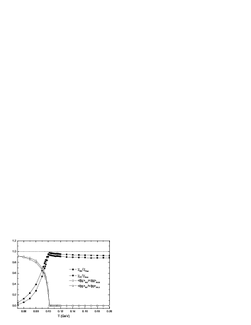
Figure 5: Temperature dependence of the QNS and the chiral condensate.

Figure 6: The QNS in the range $T>200$ MeV

V Summary

In summary, we calculate the QNS of QCD at finite temperature using both RL and BC-type truncation schemes of DSEs approach. Our result shows that when $T<T_{c}$, the QNS increases with increasing $T$ and the rate of increasing also increases with $T$. At $T_{c}$ the derivative of QNS with respect to $T$ undergoes a sudden change (from positive value to negative value). Such a behavior can be regarded as the signal of chiral phase transition. When $T_{c}<T\lesssim 200$ MeV, the QNS decreases slowly with increasing $T$. When $T$ is larger than about $200$ MeV, the QNS again increases very slowly towards the free quark gas limit with increasing $T$, which is the result of asymptotic freedom of QCD. When $T\gtrsim 95$ MeV, the difference between the QNS obtained using RL truncation and the one obtained using BC-type truncation is small ($<10\%$), which shows that the dressing effect of the quark-gluon vertex on the QNS is small. In addition, from our study it is found that for both RL and BC truncation schemes, the bahavior of the QNS across the phase transition point is nonmonotonic. Such a nonmonotonic behavior of QNS around $T_{c}$ obtained in our model differs from the existing lattice results of Refs. L5 ; L6 where a monotonic behavior of the QNS across the phase transition point is found. This difference deserves further study. Finally, we want to stress that the method used in the present paper can be generalized to the case of both finite temperature and finite chemical potential and be used to investigate the properties of the critical end point and the phase diagram of QCD.

Appendix A Expressions of the BC-type kernel

From general Lorentz analysis one can find the vector vertex $\Gamma_{\mu}(p_{k},0)$ has the following structure ($i=1,2,3$)

$$\Gamma_{i}(p_{k},0) = E_{0}\gamma_{i}+p_{i}[E_{1}\vec{\gamma}\cdot\vec{p}+E_{2}\omega_{k}\gamma_{4}-iE_{3}]$$ (31)

$$\Gamma_{4}(p_{k},0) = \tilde{F}_{0}\gamma_{4}+\omega_{k}(F_{1}\vec{\gamma}\cdot\vec{p}+\tilde{F}_{2}\omega_{k}\gamma_{4}-iF_{3})$$ (32)

$$= \omega_{k}(F_{1}\vec{\gamma}\cdot\vec{p}+F_{2}\omega_{k}\gamma_{4}-iF_{3})$$ (33)

where $F_{2}\equiv\tilde{F}_{2}+\tilde{F}_{0}/\omega_{k}^{2}$, $E_{0},\ldots,E_{3}$ and $\tilde{F}_{0},F_{1},\tilde{F}_{2},F_{2},F_{3}$ are scalar functions of $\vec{p}^{2}$ and $\omega_{k}^{2}$. For the free field case, $E_{0}=\tilde{F}_{0}=1$, $E_{1}=E_{2}=E_{3}=F_{1}=\tilde{F}_{2}=F_{3}=0$ and hence $F_{2}=1/\omega_{k}^{2}$.

From Eq. (30) the four-point Schwinger function $\Lambda_{\mu\sigma}(p_{k},q_{n};0)$ can be written as follows ($i,j=1,2,3$)

$$i\Lambda_{ij}(p_{k},q_{n};0) = \frac{(p_{j}+q_{j})}{2}\Big{[}2\Delta_{E_{0}}\gamma_{i}+\Delta_{E_{1}}(p_{i}\vec{\gamma}\cdot\vec{p}+q_{i}\vec{\gamma}\cdot\vec{q})+\Delta_{E_{2}}(p_{i}\omega_{k}+q_{i}\omega_{n})\gamma_{4}$$ (34)

$${}-i\Delta_{E_{3}}(p_{i}+q_{i})\Big{]}+\Sigma_{E_{1}}\left[\frac{p_{i}+q_{i}}{2}\gamma_{j}+\frac{\vec{\gamma}\cdot(\vec{p}+\vec{q})}{2}\delta_{ij}\right]$$

$${}+\Sigma_{E_{2}}\frac{\omega_{k}+\omega_{n}}{2}\gamma_{4}\delta_{ij}-i\Sigma_{E_{3}}\delta_{ij}$$

$$i\Lambda_{i4}(p_{k},q_{n};0) = \frac{\omega_{k}+\omega_{n}}{2}\Big{[}2\Delta_{E_{0}}\gamma_{i}+\Delta_{E_{1}}(p_{i}\vec{\gamma}\cdot\vec{p}+q_{i}\vec{\gamma}\cdot\vec{q})+\Delta_{E_{2}}(p_{i}\omega_{k}+q_{i}\omega_{n})\gamma_{4}$$ (35)

$${}-i\Delta_{E_{3}}(p_{i}+q_{i})\Big{]}+\Sigma_{E_{2}}\frac{p_{i}+q_{i}}{2}\gamma_{4}$$

$$i\Lambda_{4i}(p_{k},q_{n};0) = \frac{p_{i}+q_{i}}{2}\Big{[}\Delta_{F_{1}}(\omega_{k}\vec{\gamma}\cdot\vec{p}+\omega_{n}\vec{\gamma}\cdot\vec{q})+\Delta_{F_{2}}(\omega_{k}^{2}+\omega_{n}^{2})\gamma_{4}$$ (36)

$${}-i\Delta_{F_{3}}(\omega_{k}+\omega_{n})\Big{]}+\Sigma_{F_{1}}\frac{\omega_{k}+\omega_{n}}{2}\gamma_{i}$$

$$i\Lambda_{44}(p_{k},q_{n};0) = \frac{\omega_{k}+\omega_{n}}{2}\Big{[}\Delta_{F_{1}}(\omega_{k}\vec{\gamma}\cdot\vec{p}+\omega_{n}\vec{\gamma}\cdot\vec{q})+\Delta_{F_{2}}(\omega_{k}^{2}+\omega_{n}^{2})\gamma_{4}$$ (37)

$${}-i\Delta_{F_{3}}(\omega_{k}+\omega_{n})\Big{]}+\Sigma_{F_{1}}\frac{\vec{\gamma}\cdot(\vec{p}+\vec{q})}{2}+\Sigma_{F_{2}}(\omega_{k}+\omega_{n})\gamma_{4}-i\Sigma_{F_{3}}$$

References

- (1) P. Braun-Munzinger and J. Wambach, Colloquium: Phase diagram of strongly interacting matter, Rev. Mod. Phys. 81 (2009) 1031.
- (2) S. Gottlieb, W. Liu, D. Toussaint, R. L. Renken, and R. L. Sugar, Quark-number susceptibility of high-temperature QCD, Phys. Rev. Lett. 59 (1987) 2247.
- (3) L. McLerran,Chiral-symmetry order parameter, the lattice, and nucleosynthesis, Phys. Rev. D 36 (1987) 3291.
- (4) R. V. Gavai, J. Potvin, and S. Sanielevici, Quark-number susceptibility in quenched quantum chromodynamics, Phys. Rev. D 40 (1989) 2743.
- (5) T. Kunihiro, Quark-number susceptibility and fluctuations in the vector channel at high temperatures, Phys. Lett. B 271 (1991) 395.
- (6) S. Jeon, and V. Koch, Charged particle ratio fluctuation as a signal for quark-gluon plasma, Phys. Rev. Lett. 85 (2000) 2076.
- (7) M. Asakawa, U. Heinz, and B. Müller, Fluctuation probes of quark deconfinement, Phys. Rev. Lett. 85 (2000) 2072.
- (8) Y. Hatta and T. Ikeda, Universality, the QCD critical and tricritical point, and the quark number susceptibility, Phys. Rev. D 67 (2003) 014028.
- (9) H. Fujii, Scalar density fluctuation at the critical end point in the Nambu-Jona-Lasinio model, Phys. Rev. D 67 (2003) 094018.
- (10) H. Fujii and M. Ohtani, Sigma and hydrodynamic modes along the critical line, Phys. Rev. D 70 (2004) 014016.
- (11) S. Gottlieb, W. Liu, R. L. Renken, R. L. Sugar, and D. Toussaint, Fermion-number susceptibility in lattice gauge theory, Phys. Rev. D 38 (1988) 2888.
- (12) R. V. Gavai, and S. Gupta, Quark number susceptibilities, strangeness, and dynamical confinement, Phys. Rev. D 64 (2001) 074506.
- (13) R. V. Gavai, and S. Gupta, Continuum limit of quark number susceptibilities, Phys. Rev. D 65 (2002) 094515.
- (14) R. V. Gavai, S. Gupta, and P. Majumdar, Susceptibilities and screening masses in two flavor QCD, Phys. Rev. D 65 (2002) 054506.
- (15) C. R. Allton, S. Ejiri, S. J. Hands, O. Kaczmarek, F. Karsch, E. Laermann, and C. Schmidt, Equation of state for two flavor QCD at nonzero chemical potential, Phys. Rev. D 68 (2003) 014507.
- (16) C. R. Allton, M. Dring, S. Ejiri, S. J. Hands, O. Kaczmarek, F. Karsch, E. Laermann, and K. Redlich, Thermodynamics of two flavor QCD to sixth order in quark chemical potential, Phys. Rev. D 71 (2005) 054508.
- (17) C. Sasaki, B. Friman, and K. Redlich, Quark number fluctuations in a chiral model at finite baryon chemical potential, Phys. Rev. D 75 (2007) 054026.
- (18) J.-P. Blaizot, E. Iancu, and A. Rebhan, Quark number susceptibilities from the HTL-resummed thermodynamics, Phys. Lett. B 523 (2001) 143.
- (19) P. Chakraborty, M. G. Mustafa, and M. H. Thoma, Quark number susceptibility in hard thermal loop approximation, Eur. Phys. J. C 23 (2002) 591.
- (20) J.-P. Blaizot, E. Iancu, and A. Rebhan, Comparing different hard-thermal-loop approaches to quark number susceptibilities, Eur. Phys. J. C 27 (2003) 433.
- (21) Y. Jiang, H. X. Zhu, W. M. Sun, and H. S. Zong, The quark number susceptibility in the hard-thermal-loop approximation, J. Phys. G: Nucl. Part. Phys. 37 (2010) 055001.
- (22) Y. Jiang, H. Li, S. X. Huang, W. M. Sun, and H. S. Zong, The equation of state and quark number susceptibility in the hard-dense-loop approximation, J. Phys. G: Nucl. Part. Phys. 37 (2010) 105004.
- (23) M. He, D. K. He, H. T. Feng, W. M. Sun, and H. S. Zong, Continuum study of quark-number susceptibility in an effective interaction model, Phys. Rev. D 76 (2007) 076005.
- (24) M. He, J. F. Li, W. M. Sun, and H. S. Zong, Quark number susceptibility around the critical end point, Phys. Rev. D 79 (2009) 036001.
- (25) D. K. He, X. X. Ruan, Y. Jiang, W. M. Sun, and H. S. Zong, A model study of quark-number susceptibility at finite chemical potential and temperature, Phys. Lett. B 680 (2009) 432.
- (26) P. Maris, and C. D. Roberts, - and - meson Bethe-Salpeter amplitudes, Phys. Rev. C 56 (1997) 3369.
- (27) P. Maris, and P. C. Tandy, Bethe-Salpeter study of vector meson masses and decay constants, Phys. Rev. C 60 (1999) 055214.
- (28) J. C. R. Bloch, Multiplicative renormalizability and quark propagator, Phys. Rev. D 66 (2002) 034032.
- (29) P. Maris, A. Raya, C. D. Roberts, and S. M. Schmidt, Facets of confinement and dynamical chiral symmetry breaking, Eur. Phys. J. A 18 (2003) 231.
- (30) G. Eichmann, R. Alkofer, I. C. Cloët, A. Krassnigg, and C. D. Roberts, Perspective on rainbow-ladder truncation, Phys. Rev. C 77 (2008) 042202 (R).
- (31) G. Eichmann, I. C. Cloët, R. Alkofer, A. Krassnigg, and C. D. Roberts, Toward unifying the description of meson and baryon properties, Phys. Rev. C 79 (2009) 012202 (R).
- (32) A. Höll, C. D. Roberts, and S. V. Wright, Hadron physics and Dyson-Schwinger equations, [arxiv: nucl-th/0601071v1] (2006).
- (33) J. S. Ball, and T. W. Chiu, Analytic properties of the vertex function in gauge theories. I, Phys. Rev. D 22 (1980) 2542.
- (34) J. S. Ball, and T. W. Chiu, Analytic properties of the vertex function in gauge theories. II, Phys. Rev. D 22 (1980) 2550.
- (35) D. C. Curtis, and M. R. Pennington, Truncating the Schwinger-Dyson equations: How multiplicative renormalizability and the Ward identity restrict the three point vertex in QED, Phys. Rev. D 42 (1990) 4165.
- (36) H. X. He, and F. C. T. Khanna, Transverse Ward-Takahashi identity for the fermion boson vertex in gauge theories, Phys. Lett. B 480 (2000) 222.
- (37) H. X. He, Identical relations among transverse parts of variant Green functions and the full vertices in gauge theories, Phys. Rev. C 63 (2001) 025207.
- (38) H. X. He, Transverse symmetry transformations and the quark-gluon vertex function in QCD, Phys. Rev. D 80 (2009) 016004.
- (39) W. Marciano, and H. Pagels, Quantum chromodynamics: A review, Phys. Rept. 36 (1978) 137.
- (40) L. Chang, and C. D. Roberts, Sketching the Bethe-Salpeter kernel, Phys. Rev. Lett. 103 (2009) 081601.
- (41) W. M. Sun, and H. S. Zong, A general method for calculating partition function of QCD at finite chemical potential, Int. J. Mod. Phys. A 22 (2007) 3201.
- (42) M. He, W. M. Sun, H. T. Feng, and H. S. Zong, A model study of QCD phase transition, J. Phys G: Nucl. Part. Phys. 34 (2007) 2655.
- (43) M. He, Y. Jiang, W. M. Sun, and H. S. Zong, Chiral susceptibility in an effective interaction model, Phys. Rev. D 77 (2008) 076008.
- (44) C. D. Roberts, and S. M. Schmidt, Dyson-Schwinger equations: Density, temperature and continuum strong QCD, Prog. Part. Nucl. Phys. 45 (2000) S1.
- (45) A. Höll, P. Maris, and C. D. Roberts, Mean field exponents and small quark mass, Phys. Rev. C 59 (1999) 1751.
- (46) C. D. Roberts, and A. G. Williams, Dyson-Schwinger equations and their application to hadron physics, Prog. Part. Nucl. Phys. 33 (1994) 477.
- (47) P. Maris, C. D. Roberts, S. M. Schmidt, and P. C. Tandy, T dependence of pseudoscalar and scalar correlations, Phys. Rev. C 63 (2001) 025202.
- (48) H. J. Munczek, Dynamical chiral symmetry breaking, Goldstone’s theorem, and the consistency of the Schwinger-Dyson and Bethe-Salpeter equations, Phys. Rev. D 52 (1995) 4736.
- (49) A. Bender, C. D. Roberts, and L. V. Smekal, Goldstone theorem and diquark confinement beyond rainbow-ladder approximation, Phys. Lett. B 380 (1996) 7.
- (50) L. Chang, Y. X. Liu, C. D. Roberts, Y. M. Shi, W. M. Sun, and H. S. Zong, Chiral susceptibility and the scalar Ward identity, Phys. Rev. C 79 (2009) 035209.
- (51) Y. M. Shi, H. X. Zhu, W. M. Sun, and H. S. Zong, Calculation of tenson susceptibility beyond rainbow-ladder approximation, Few-Body Syst. 48 (2010) 31.
- (52) M. Cheng, et.al., Transition temperature in QCD, Phys. Rev. D 74 (2006) 054507.