Gauge-flation: Inflation From Non-Abelian Gauge Fields

Abstract

Inflationary models are usually based on dynamics of one or more scalar fields coupled to gravity. In this work we present a new class of inflationary models, gauge-flation or non-Abelian gauge field inflation, where slow-roll inflation is driven by a non-Abelian gauge field. This class of models are based on a gauge field theory with a generic non-Abelian gauge group minimally coupled to gravity. We then focus on a particular gauge-flation model by specifying the action for the gauge theory. This model has two parameters which can be determined using the current cosmological data and has the prospect of being tested by Planck satellite data. Moreover, the values of these parameters are within the natural range of parameters in generic grand unified theories of particle physics.

Inflationary Universe paradigm Inflation-Books ; Weinberg , the idea that early Universe has undergone an inflationary (accelerated expansion) phase, has appeared very successful in reproducing the current cosmological data through the $\Lambda$CDM model Inflation-Books ; Weinberg . Many models of inflation have been proposed and studied so far, e.g. see Bassett-review , which are all compatible with the current data. Inflationary models are generically single or multi scalar field theories with standard or non-standard kinetic terms and a potential term, which are minimally or non-minimally coupled to gravity. Generically, in these models inflationary period is driven by a “slowly rolling” scalar field (inflaton field) whose kinetic energy remains small compared to the potential terms.

Toward the end of inflation the kinetic term becomes comparable to the potential energy, and inflaton field(s) start a (fast) oscillation around the minimum of their potential losing their energy to other fields present in the theory, the (p)reheating period. The energy of the inflaton field(s) should eventually be transferred to standard model particles, reheating, where standard FRW cosmologies take over. Therefore, to have a successful cosmology model one should embed the model into particle physics models. With the current data the scale of inflation (or Hubble parameter $H$ during inflation) is not restricted well enough, it can range from $10^{14}$ GeV to the Bing Bang Nucleosynthesis scale $1$ MeV. However, larger $H$, $H\gtrsim 10$ GeV, is preferred within the slow-roll inflationary models with preliminary particle or high energy physics considerations. It is hence natural to tune the inflationary model within the existing particle physics models suitable for similar energy scales.

Most of successful inflationary scenarios so far use scalar field(s) as the inflaton, because turning on time dependent scalar fields does not spoil the homogeneity and isotropy of the cosmology. Although it is relatively easy to write down a potential respecting the slow-roll dynamics conditions, it is generically not easy to argue for such potentials and their stability against quantum corrections within particle physics models. For example, the Higgs sector in the ordinary electroweak standard model minimally coupled to Einstein gravity does not support a successful inflationary model e.g. see Higgs-inflation . The situation within beyond standard model theories seems not to be better.

Vector gauge fields are commonplace in all particle physics models. However, their naive usage in constructing inflationary models is in clash with the homogeneity and isotropy of the background. It has been argued that this obstacle may be overcome by introducing many vector fields which contribute to the inflation, such that the anisotropy induced by them all average out vector-inflation . Alternatively one may introduce three orthogonal vector fields and retain rotational invariance by identifying each of these fields with a specific direction in space vector-inflation . Nonetheless, it was shown that it is not possible to get a successful vector inflation model in a gauge invariant setting vector-inflation . Lack of gauge invariance, once quantum fluctuations are considered may lead to instability of the background and may eventually invalidate the background classical inflationary dynamics analysis vector-inflation-loophole .

Here, we construct a new class of vector inflation models and to avoid the above mentioned possible instability issue we work in the framework of gauge field theories. In addition, to remove the incompatibility with isotropy resulting from gauge fields we introduce three gauge fields. We choose these gauge fields to rotate among each other by $SU(2)$ non-Abelian gauge transformations. Explicitly, the rotational symmetry in 3d space is retained because it is identified with the global part of the $SU(2)$ gauge symmetry. In our model we need not restrict ourselves to $SU(2)$ gauge theory and, since any non-Abelian gauge group has an $SU(2)$ subgroup, our gauge-flation (non-Abelian gauge field inflation) model can be embedded in non-Abelian gauge theories with arbitrary gauge group. Another advantage of using non-Abelian gauge theories is that, due to the structure of non-Abelian gauge field strength, there is always a potential induced for the combination of the gauge field components which effectively plays the role of the inflaton field.

In the above discussions we have only committed ourselves to the gauge invariance and have not fixed a specific gauge theory action. This action will be fixed on the requirement of having a successful inflationary model. We study one such gauge-flation model but gauge-flation models are expected not to be limited to this specific choice. In this Letter we consider a simple two parameter gauge-flation model and study classical inflationary trajectory for this model as well as the cosmic perturbation theory around the inflationary path. We then use the current data for constraining the parameters of our model and show that our model is compatible with the current data within a natural range for its parameters.

The inflationary setup. Consider a 4-dimensional $su(2)$ gauge field $A^{a}_{~{}\mu}$, where $a,b,...$ and $\mu,\nu,...$ are respectively used for the indices of the gauge algebra and the space-time. We will be interested in gauge invariant Lagrangians ${\cal L}(F^{a}_{~{}\mu\nu},g_{\mu\nu})$ which are constructed out of metric $g_{\mu\nu}$ and the strength field $F$

$$F^{a}_{~{}\mu\nu}=\partial_{\mu}A^{a}_{~{}\nu}-\partial_{\nu}A^{a}_{~{}\mu}-g\epsilon^{a}_{~{}bc}A^{b}_{~{}\mu}A^{c}_{~{}\nu},$$ (1)

where $\epsilon_{abc}$ is the totally antisymmetric tensor. We work with FRW inflationary background metric

$$ds^{2}=-dt^{2}+a(t)^{2}\delta_{ij}dx^{i}dx^{j},$$ (2)

where indices $i,j,...$ label the spatial directions.

The effective inflaton field is introduced as follows: We will work in temporal gauge $A^{a}_{~{}0}=0$ and at the background level, as in any inflationary model, we only allow for $t$ dependent field configurations Galtsov

$$A^{a}_{~{}\mu}=\left\{\begin{array}[]{ll}\phi(t)\delta^{a}_{i}\,,&\mu=i\\ 0\,,&\mu=0\,.\end{array}\right.$$ (3)

With this choice we are actually identifying our gauge indices with the spatial indices. That is, we identify the rotation group $SO(3)$ with the global part of the gauge group, $SU(2)$. Therefore, the rotational non-invariance resulted from turning on space components of a vector is compensated by (the global part of) the gauge symmetry. $\phi(t)$ is not a genuine scalar, while

$$\psi(t)=\frac{\phi(t)}{a(t)}$$ (4)

is indeed a scalar. (Note that for the flat FRW metric $e^{a}_{~{}i}=a(t)\delta^{a}_{i}$ , where $e^{a}_{~{}i}$ are the 3d triads.) The components of the field strengths in the ansatz are

$$F^{a}_{~{}0i}=\dot{\phi}\delta^{a}_{i}\,,\qquad F^{a}_{~{}ij}=-g\phi^{2}\epsilon^{a}_{~{}ij}.$$ (5)

After fixing the gauge and choosing $A^{a}_{~{}0}$ to be zero, system has nine other degrees of freedom, $A^{a}_{~{}i}$. However, in the ansatz (3) we only keep one scalar degree of freedom. We should hence first discuss consistency of the reduction ansatz (3) with the classical dynamics of the system induced by ${\cal L}(F^{a}_{~{}\mu\nu},g_{\mu\nu})$. It is straightforward to show that the gauge field equations of motion $D_{\mu}\frac{\partial{\cal L}}{\partial F_{\mu\nu}}=0$, where $D_{\mu}$ is the gauge covariant derivative, i) allows for a solution of the form (3) and, ii) once evaluated on the ansatz (3) becomes equivalent to the equation of motion obtained from the “reduced Lagrangian” ${\cal L}_{\textrm{red}}(\dot{\phi},\phi;a(t))$,

$$\frac{d}{a^{3}dt}(a^{3}\frac{\partial{\cal L}_{red.}}{\partial\dot{\phi}})-\frac{\partial{\cal L}_{red.}}{\partial\phi}=0\,,$$ (6)

where ${\cal L}_{red.}$ is obtained from inserting (5) and metric (2) into the original gauge theory Lagrangian ${\cal L}$. Moreover, one can show that the energy momentum tensor, $T_{\mu\nu}$, computed over the FRW background (2) and the gauge field ansatz (3) takes the form of a homogeneous perfect fluid

$$T^{\mu}_{\ \nu}=diag(-\rho,P,P,P)\,,$$

which is the same as the energy momentum tensor obtained from the reduced Lagrangian ${\cal L}_{\textrm{red}}$. That is,

$$\rho=\frac{\partial\mathcal{L}_{red.}}{\partial\dot{\phi}}\dot{\phi}-\mathcal{L}_{red.}\,,\qquad P=\frac{\partial(a^{3}{\cal L}_{red.})}{\partial a^{3}}\ .$$ (7)

All the above is true for any gauge invariant Lagrangian ${\cal L}={\cal L}(F_{\mu\nu}^{a};g_{\mu\nu})$. To have a successful inflationary model, however, we should now choose appropriate form of ${\cal L}$. The first obvious choice is Yang-Mills action minimally coupled to Einstein gravity. This will not lead to an inflating system with $\rho+3P<0$, because as a result of scaling invariance of Yang-Mills action one immediately obtains $P=\rho/3$ and that $\rho\geq 0$. So, we need to consider modifications to Yang-Mills. As will become clear momentarily one such appropriate choice is

$$S=\int d^{4}x\sqrt{-{g}}\left[-\frac{R}{2}-\frac{1}{4}F^{a}_{~{}\mu\nu}F_{a}^{~{}\mu\nu}+\frac{\kappa}{384}(\epsilon^{\mu\nu\lambda\sigma}F^{a}_{~{}\mu\nu}F^{a}_{~{}\lambda\sigma})^{2}\right]\,$$ (8)

where we have set $8\pi G\equiv M_{\rm pl}^{-2}=1$ and $\epsilon^{\mu\nu\lambda\sigma}$ is the totally antisymmetric tensor. This specific $F^{4}$ term is chosen because the contribution of this term to the energy momentum tensor will have the equation of state $P=-\rho$, making it perfect for driving inflationary dynamics. (To respect the weak energy condition for the $F^{4}$ term, we choose $\kappa$ to be positive.) The reduced (effective) Lagrangian is obtained from evaluating (8) for the ansatz (3):

$$\mathcal{L}_{red}=\frac{3}{2}(\frac{\dot{\phi}^{2}}{a^{2}}-\frac{g^{2}\phi^{4}}{a^{4}}+\kappa\frac{g^{2}\phi^{4}\dot{\phi}^{2}}{a^{6}}).$$ (9)

Energy density $\rho$ and pressure $P$ are then given by

$$\rho=\rho_{{}_{YM}}+\rho_{\kappa}\ ,\qquad P=\frac{1}{3}\rho_{{}_{YM}}-\rho_{\kappa},$$ (10)

where

$$\rho_{{}_{YM}}=\frac{3}{2}(\frac{\dot{\phi}^{2}}{a^{2}}+\frac{g^{2}\phi^{4}}{a^{4}})\ ,\qquad\rho_{\kappa}=\frac{3}{2}\kappa\frac{g^{2}\phi^{4}\dot{\phi}^{2}}{a^{6}}\,.$$ (11)

Recalling the Friedmann equations

$$\begin{split}H^{2}&=\frac{1}{2}(\frac{\dot{\phi}^{2}}{a^{2}}+\frac{g^{2}\phi^{4}}{a^{4}}+\kappa\frac{g^{2}\phi^{4}\dot{\phi}^{2}}{a^{6}}),\cr\dot{H}~{}&=-(\frac{\dot{\phi}^{2}}{a^{2}}+\frac{g^{2}\phi^{4}}{a^{4}})\,,\end{split}$$ (12)

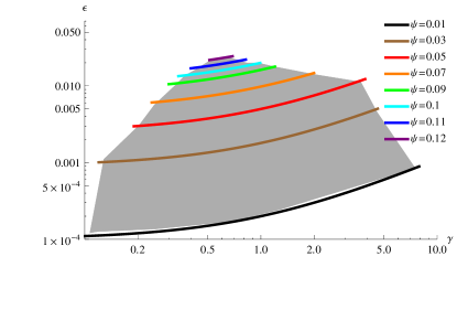
the slow-roll parameter $\epsilon$ is

$$\epsilon=-\frac{\dot{H}}{H^{2}}=\frac{2\rho_{{}_{YM}}}{\rho_{{}_{YM}}+\rho_{\kappa}}\,.$$ (13)

To obtain a slow-roll inflationary phase initial conditions and parameter $\kappa$ should be chosen such that $\rho_{\kappa}$ dominates over $\rho_{{}_{YM}}$ during inflation. As slow-roll inflation progresses the contribution of Yang-Mills term $\rho_{{}_{YM}}$ to the energy momentum tensor grows and eventually at around $\rho_{{}_{YM}}=\rho_{\kappa}$ inflation ends. To have a consistent slow-roll inflation, it is not sufficient to have small $\epsilon$; for any physical quantity $X$, $\frac{\dot{X}}{HX}$ should remain small. In particular, demanding the effective scalar inflaton field $\psi$ to be slowly varying, i.e. $\delta\equiv-\frac{\dot{\psi}}{H\psi}\ll 1$ and $\dot{\delta}/(H\delta)\ll 1$, yields

$$\epsilon \simeq\psi^{2}(1+\gamma),\quad\eta\simeq\psi^{2}$$ (14a)

$$\delta \simeq\frac{\gamma}{6(\gamma+1)}\epsilon^{2},\quad\kappa\simeq\frac{(2-\epsilon)(1+\gamma)^{3}}{g^{2}\epsilon^{3}},$$ (14b)

in the leading order in $\epsilon$. In the above

$$\gamma=\frac{g^{2}\psi^{2}}{H^{2}}\quad\textrm{or equivalently}\quad H^{2}\simeq\frac{g^{2}\epsilon}{\gamma(\gamma+1)}\,,$$ (15)

$\gamma$ is a slowly varying positive parameter of order one. Since $\delta\sim\epsilon^{2}$ (cf. (14b)), $\psi$ is varying slower than $\epsilon$ and hence from (15) we learn that during slow-roll regime

$$\frac{\epsilon}{\epsilon_{i}}\simeq\frac{\gamma+1}{\gamma_{i}+1}\,,\quad\frac{\gamma}{\gamma_{i}}\simeq\frac{H_{i}^{2}}{H^{2}}\,,$$ (16)

where $\epsilon_{i},\ \gamma_{i}$ and $H_{i}$ are the values of these parameters at the beginning of inflation. Number of e-folds $N_{e}$ at the end of inflation, marked by $\epsilon_{f}=1$, is then given by

$$N_{e}=\int_{t_{i}}^{t_{f}}Hdt=-\int_{H_{i}}^{H_{f}}\frac{dH}{\epsilon H}\simeq\frac{\gamma_{i}+1}{2\epsilon_{i}}\ln\frac{\gamma_{i}+1}{\gamma_{i}}\,.$$ (17)

The value of $\psi$ at the beginning and end of inflation are related as $\psi_{f}^{6}\simeq\frac{1}{2}\psi_{i}^{6}$, where (14b) has been used and by $\simeq$ sign we mean equality to the leading order in slow-roll parameter $\epsilon$. Notice that all the dimensionful quantities, like $\kappa,\ \psi$ and $H$, are measured in units of $M_{\rm pl}$.

Gauge-flation cosmic perturbation theory. Sofar we have analyzed dynamics of the homogeneous effective scalar inflaton field $\psi$, while consistently turning off the other gauge field components. To compare our model with the data we should work out the power spectrum of curvature perturbations and their spectral tilt for which we need to study cosmic perturbation theory in gauge-flation. In general small fluctuation around the ansatz (3) can be parameterized by 12 fields $\delta A_{\mu}^{a}$. Decomposing $\mu$ index into time and spatial parts and identifying the gauge index $a$ with the spatial index $i$, these 12 fields give rise to four scalars, three divergence-free vectors and a divergence-free, traceless symmetric tensor:

$$\delta A^{a}_{~{}0} = \delta^{ak}\partial_{k}\dot{Y}+\delta^{a}_{j}u^{j},$$

$$\delta A^{a}_{~{}i} = \delta^{a}_{i}Q+\delta^{aj}\partial_{ij}(M+\partial_{i}v_{j}+t_{ij})+\epsilon^{a~{}j}_{~{}i}(g\phi\partial_{j}P+w_{j}),$$

where $\partial_{i}$ denotes partial derivative respect to $x^{i}$, the scalars are parameterized by $Y,Q,M,P$, vectors by $u_{i},v_{i},\ w_{i}$ and the tensor by $t_{ij}$. As we see, we are indeed dealing with a multi-field inflationary model. Among the scalars, $Q$ can be identified with the fluctuation of the inflaton field $\phi$.

The other field active during inflation is metric whose fluctuations are customarily parameterized by four scalars, two divergence-free vectors and one tensor:

$$ds^{2}=-(1+2A)dt^{2}+2a(\partial_{i}B-S_{i})dx^{i}dt$$

$$+ a^{2}\left((1-2C)\delta_{ij}+2\partial_{ij}E+2\partial_{(i}W_{j)}+h_{ij}\right)dx^{i}dx^{j}.\,\,\,$$

In the first order perturbation theory which we are interested in, scalar, vector and tensor fluctuations do not couple to each other. Among 12 gauge field perturbations and 10 metric perturbations one scalar and one vector mode of the gauge field, and two scalars and one vector of the metric modes are gauge degrees of freedom. We hence remain with five gauge-invariant scalar, three massless vector and two massless tensor modes.

Figure 1: In the left panel we have depicted ${P_{{}_{R}}}+{P_{{}_{L}}}$. In the standard scalar-driven inflationary models ${P_{{}_{R}}}={P_{{}_{L}}}=1$. The right panel the parity violating factor $\frac{P_{{}_{R}}-P_{{}_{L}}}{P_{{}_{R}}+P_{{}_{L}}}$ versus $\gamma$ for $\psi=10^{-2}$ and $\psi=0.12$ is shown. The power spectra have been calculated at $k\tau=-0.01$, long enough after modes have crossed the horizon and behave quite classically. As we see in the right panel, for very small and very large $\gamma$ values $P_{{}_{R}}\gg P_{{}_{L}}$.

Equations of motion for the perturbations can be obtained from perturbed Einstein equations $\delta G_{\mu\nu}=\delta T_{\mu\nu},$ which decomposes into four equations for scalar modes, two for vector modes and one equation for tensor modes Weinberg . The equation of motion for the remaining scalar, vector and tensor mode $t_{ij}$ is provided through perturbed gauge field equations.

A thorough analysis reveals that amplitude of vector perturbations are exponentially suppressed, as in the ordinary scalar-driven inflationary models gauge-flation-prd . Although the tensor mode perturbations in the gauge field sector $t_{ij}$ are suppressed at the superhorizon scales, their presence leads to parity violating terms in the second order action governing the metric tensor perturbations $h_{ij}$ gauge-flation-prd . This happens due to the fact that one of two modes of $t_{ij}$ (say, the right-handed circular polarization) just before the horizon-crossing undergoes a tachynoic growth for a short period and as a result the right-handed circular polarization of $h_{ij}$ becomes large at superhorizon value. On the other hand, the left-handed polarization of $t_{ij}$ remains small at horizon-crossing and has negligible effect on the superhorizon value of its corresponding $h_{ij}$ polarization.

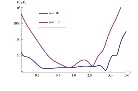
The power spectra for the Left and Right gravitational wave modes are obtained as gauge-flation-prd

$$\mathcal{P}_{T_{R}}\simeq P_{{}_{R}}\left(\frac{H}{\pi}\right)^{2}\!\!\big{|}_{k=aH}\quad\&\quad\mathcal{P}_{T_{L}}\simeq P_{{}_{L}}\left(\frac{H}{\pi}\right)^{2}\!\!\big{|}_{k=aH}\,,$$

where $P_{{}_{R}}$ and $P_{{}_{L}}$ are functions of the parameters $\gamma,\psi$ (Fig.1). The power spectrum of the tensor modes, is then given as $\mathcal{P}_{T}=\mathcal{P}_{T_{R}}+\mathcal{P}_{T_{L}}$.

The full analysis of cosmic perturbation theory in our model has many new and novel features compared to the standard scalar-driven inflationary models, a detailed analysis of which is presented in gauge-flation-prd , in the following table we summarize the results:

Power spectrum of curvature perturbations	$\mathcal{P}_{\mathcal{R}}$	$\frac{1}{8\pi^{2}\epsilon}\left(\frac{H}{M_{\rm pl}}\right)\!^{2}$
Spectral Tilt	$n_{s}-1$	$\hskip 5.69046pt-2(\epsilon-\eta)$
Tensor to Scalar ratio	$r$	$8(P_{{}_{R}}+P_{{}_{L}})\epsilon$
Power spectrum of anisotropic inertia $a^{2}\!\pi^{S}$	$\mathcal{P}_{\!a^{2}\!\pi^{S}}$	$\frac{\epsilon}{8\pi^{2}}\left(\frac{H}{M_{\rm pl}}\right)\!^{2}$

A specific feature of gauge-flation is that it predicts a non-zero power spectrum for the scalar anisotropic inertia $a^{2}\!\pi^{S}$ Weinberg , with the ratio

$$\frac{\mathcal{P}_{\!a^{2}\!\pi^{S}}}{\mathcal{P}_{\mathcal{R}}}=\epsilon^{2}\,.$$ (18)

Note that $a^{2}\!\pi^{S}$ is identically zero in all the scalar-driven inflationary models in the context of Einstein GR.

Confronting gauge-flation with the data. To this end, we depict the results of our model on the allowed region of the $n_{s}-r$ graph:

Figure 2: The left panel shows $1\sigma$ and $2\sigma$ contour bounds of 7-year WMAP+BAO+H0. The yellow area (region with lighter color) represents the gauge-flation predictions for $\psi\in(0.01,0.12)$ range. The region with enough number of e-folds restricts us to $n_{s}>0.98$ region, that is on the right-side of the $N_{e}=50$ line gauge-flation-prd . Therefore, the allowed region is the highlighted region between $N_{e}=50$ and $n_{s}=1$ lines. The shaded region in right panel shows the allowed values for $\epsilon$ and $\psi$.

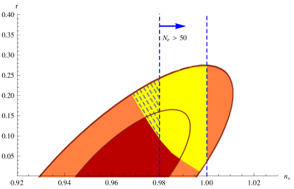
From the left panel of Figs 2, we learn that in the allowed region the value of $\gamma$ is restricted as $\gamma\in(0.1-8)$ which determines the value of $\kappa$ and $g$

$$\begin{split}g&\simeq(0.15-3.7)\times 10^{-3},\cr\Lambda&\sim(10^{-5}-10^{-4})M_{\rm pl}\,,\quad\kappa\equiv\Lambda^{-4}\,.\end{split}$$ (19)

Restricting ourselves to $1\sigma$ contour in Fig 2, we find stringent bounds on $r$, $n_{\mathcal{R}}$, $\frac{\mathcal{P}_{\!a^{2}\!\pi^{S}}}{\mathcal{P}_{\mathcal{R}}}$ and $H$

$$0.05< r <0.15\ ,\ \quad H\simeq(3.4-5.4)\times 10^{-5}M_{\rm pl},$$ (20)

$$0.98\leq n_{s} \leq 0.99\ ,\ \quad\frac{\mathcal{P}_{\!a^{2}\!\pi^{S}}}{\mathcal{P}_{\mathcal{R}}}\simeq(3.6-22)\times 10^{-5},$$ (21)

while within the $1\sigma$ contour, we have $0.5<\gamma<4$ and the gauge field value during inflation turns out to be sub-Planckian $\psi\simeq(0.4-1)\times 10^{-1}M_{\rm pl}$.

Discussion. We showed that non-Abelian gauge field driven inflation, gauge-flation, can lead to a successful slow-roll inflation model with specific features. In the model we considered the theory has two parameters, gauge coupling $g$ and the coefficient of the $(F\tilde{F})^{2}$ term $\kappa$. The value for the gauge coupling $g$ required by the CMB data is of order $10^{-3}$, while $\Lambda$, the scale associated with $\kappa\sim\Lambda^{-4}$, is of order $10^{14}$GeV. These two parameters are in the natural range for perturbative beyond standard models of particle physics. Moreover, the $\kappa$-term may be obtained by integrating out axionic fields where $\Lambda$ is associated with scale of the axion potential Weinberg-vol2 ; integrate-out . For this procedure to be theoretically meaningful we need $\Lambda\gg H$, which is respected by the best-fit values of our model.

Current data tightly restricts the values of our parameters. In particular, noting Fig. 2, our model predicts that the tensor-to-scalar ratio $r$ is restricted to be in $0.02<r<0.15$ range, which is well within the range to be probed by the Planck satellite. As another prediction, while gauge-flation has always a red spectral tilt, the tilt has a lower bound $n_{s}>0.98$.

Finally we point out a specific feature of our model not shared by usual scalar-driven inflationary models: gauge-flation predicts a non-zero scalar anisotropic inertia $(a^{2}\!\pi^{S}\neq 0)$, and $\frac{\mathcal{P}_{a\!^{2}\!\pi\!^{S}}}{\cal{P}_{\cal{R}}}\sim 10^{-4}$. It would be interesting to explore observational prospects this ratio, which we postpone to future works.

Note added: More than a year after appearance of the original version of this work on the arXiv, the paper AMW appeared which prompted us to recheck and correct the tensor mode sector of gauge-flation cosmic perturbation theory. A more detailed analysis may be found in gauge-flation-prd ; The-review .

Acknowledgement: We would like to thank Amjad Ashoorioon and Bruce Bassett for comments on the manuscript and Niayesh Afshordi for useful discussions and comments. Work of A.M. is partially supported by grants from Bonyad-e Melli Nokhbegan of Iran.

References

- (1) V. Mukhanov, “Physical Foundations of Cosmology,” Cambrdige Uni. Press (2005).
- (2) S. Weinberg, “Cosmology,” SPIRES entry Oxford, UK: Oxford Univ. Pr. (2008).
- (3) B. A. Bassett, S. Tsujikawa and D. Wands, “Inflation dynamics and reheating,” Rev. Mod. Phys. 78, 537 (2006), [arXiv:astro-ph/0507632].
- (4) F. L. Bezrukov and M. Shaposhnikov, “The Standard Model Higgs boson as the inflaton,” Phys. Lett. B 659, 703 (2008), [arXiv:0710.3755 [hep-th]]; J. L. F. Barbon and J. R. Espinosa, “On the Naturalness of Higgs Inflation,” Phys. Rev. D 79, 081302 (2009), [arXiv:0903.0355 [hep-ph]]; A. O. Barvinsky, A. Y. Kamenshchik and A. A. Starobinsky, “Inflation scenario via the Standard Model Higgs boson and LHC,” JCAP 0811, 021 (2008), [arXiv:0809.2104 [hep-ph]].
- (5) A. Golovnev, V. Mukhanov and V. Vanchurin, “Vector Inflation,” JCAP 0806, 009 (2008), [arXiv:0802.2068[astro-ph]].
- (6) B. Himmetoglu, C. R. Contaldi, M. Peloso, “Instability of anisotropic cosmological solutions supported by vector fields,” Phys. Rev. Lett. 102, 111301 (2009), [arXiv:0809.2779 [astro-ph]]; B. Himmetoglu, C. R. Contaldi and M. Peloso, “Instability of the ACW model, and problems with massive vectors during inflation,” Phys. Rev. D 79, 063517 (2009), [arXiv:0812.1231 [astro-ph]]. M. Karciauskas and D. H. Lyth, “On the health of a vector field with coupling to gravity,” JCAP 1011 (2010) 023, [arXiv:1007.1426 [astro-ph.CO]].
- (7) D. V. Galtsov and M. S. Volkov,“Yang-Mills cosmology: Cold matter for a hot universe,” Phys. Lett. B 256, 17 (1991).
- (8) A. Maleknejad and M. M. Sheikh-Jabbari, “Non-Abelian Gauge Field Inflation,” [arXiv:1102.1932 [hep-ph]].
- (9) E. Komatsu et al. [WMAP Collaboration], “Seven-Year Wilkinson Microwave Anisotropy Probe (WMAP) Observations: Cosmological Interpretation,” Astrophys. J. Suppl. 192, 18 (2011), [arXiv:1001.4538 [astro-ph.CO]].
- (10) S. Weinberg, “The quantum theory of fields. Vol. 2: Modern applications,” Cambridge, UK: Univ. Pr. (1996).
- (11) M. M. Sheikh-Jabbari, “Gauge-flation Vs Chromo-Natural Inflation,” Phys. Lett. B 717, 6 (2012), [arXiv:1203.2265 [hep-th]].
- (12) P. Adshead, E. Martinec and M. Wyman, “A Sinister Universe: Chiral gravitons lurking, and Lyth un-bound,” arXiv:1301.2598 [hep-th].
- (13) A. Maleknejad, M. M. Sheikh-Jabbari and J. Soda, “Gauge Fields and Inflation,” arXiv:1212.2921 [hep-th].