Electromagnetic Casimir Energies of Semi-Infinite Planes

Abstract

Using recently developed techniques based on scattering theory, we find the electromagnetic Casimir energy for geometries involving semi-infinite planes, a case that is of particular interest in the design of microelectromechanical devices. We obtain both approximate analytic formulae and exact results requiring only modest numerical computation. Using these results, we analyze the effects of edges and orientation on the Casimir energy. We also demonstrate the accuracy, simplicity, and utility of our approximation scheme, which is based on a multiple reflection expansion.

Introduction and Method

The Casimir energy has been most commonly studied using techniques based on the original calculation for infinite parallel planes Casimir48 . Recently developed techniques spheres ; universal have made it possible to calculate the electromagnetic Casimir force between objects of arbitrary shape and electromagnetic response. In recent applications of these methods, the interaction energy of a semi-infinite plane with an infinite plane was analyzed in two different ways: First, with the half-plane considered as the limit of a parabolic cylinder of zero curvature parabolic , in which case the exact energy can be computed numerically. Second, with the semi-infinite plane taken as the limit of a wedge of zero opening angle wedge , in which case it is convenient to consider a multiple reflection expansion for the energy. Remarkably, the analytic formulae obtained by keeping the lowest few orders in the reflection expansion give very good agreement with the full numerical result. (This approach can also be extended to interactions of more than two bodies Maghrebi10-2 .) We study the Casimir interaction of semi-infinite planes by contrasting these two methods. This problem is applicable to the design of microelectromechanical devices Khoshnoud and has been of recent theoretical interest as well Gies ; Kabat . We present analytic formulae obtained through the multiple-reflection approximation and use the exact numerical calculation to obtain a concrete measure of the accuracy of the approximations involved. This system provides an ideal environment in which to study the effects of edges and orientation.

In the scattering theory approach spheres ; universal , the Casimir interaction energy is expressed in terms of the scattering $T$-matrices, also known as scattering amplitudes, for each object individually. These matrices incorporate the material characteristics of each object individually, while the objects’ relative positions and orientations are described by universal translation matrices. These matrices connect the bases of wavefunctions, centered on each object, in which the scattering amplitudes are calculated. For the case of two objects that are translationally invariant in the $z$-direction, we consider the energy per unit length

$$\frac{\cal E}{\hbar cL}=\int_{0}^{\infty}\frac{d\kappa}{2\pi}\int_{-\infty}^{\infty}\frac{dk_{z}}{2\pi}\log\det\left({\mathbbm{1}}-T_{1}\,{\cal U}_{12}T_{2}\,{\cal U}_{21}\right)\,,$$ (1)

where the ${T}_{j}$ give the $T$-matrices for each object, while the ${\cal U}_{ij}={\cal U}_{ji}^{\dagger}$ give the translation matrices from one object to another. Here $k=i\kappa=\omega/c$ is the magnitude of the wave vector for each possible fluctuation and $k_{z}$ is its $z$-component. We can interpret this formula in terms of the propagation of electromagnetic fluctuations between the objects: The $T$-matrices describe the reflection of fluctuating fields from a single object, while the $U$-matrices propagate these fluctuations from one object to another. The determinant then combines all possible reflections among the objects. By evaluating the integral and determinant numerically, we can use Eq. (1) to find exact results for the Casimir interaction energy. However, this expression also allows for a systematic approximation, in which we can obtain simple analytic results. Letting ${\cal N}=T_{1}{\cal U}_{12}T_{2}{\cal U}_{21}$, we can convert the log-determinant to a trace-log, which we then expand as a Taylor series,

$$\frac{\cal E}{\hbar cL}=-\int_{0}^{\infty}\frac{d\kappa}{2\pi}\int_{-\infty}^{\infty}\frac{dk_{z}}{2\pi}\sum_{n=1}^{\infty}\frac{1}{n}{\rm tr}{\cal N}^{n}\,.$$ (2)

In this expansion, the $n^{\hbox{\tiny th}}$ term then gives the contribution from $n$ reflections (back and forth) between the two objects. These contributions typically fall at least as fast as $n^{-(D+1)}$, where $D$ is the dimension of space optical ; wedge .

We can realize the half-plane geometry as the limit of either a wedge wedge with zero opening angle or a parabolic cylinder parabolic with zero radius of curvature. In the former case the $T$-matrix is expressed in a basis indexed by continuous imaginary angular momentum $\lambda$, while in the latter case the $T$-matrix is given in a basis with discrete channels $\nu=0,1,2\ldots$. Although we can compute either the full determinant or the multiple reflection expansion using either basis, the wedge basis is better suited to the reflection expansion, because the associated translation matrix elements are simpler and easier to handle analytically, while the parabolic cylinder basis is better suited to the full determinant calculation, because it is easier to calculate the determinant when the matrix involves discrete rather than continuous indices.

Two Half-Planes

We consider two half-planes, and restrict our attention to configurations that are translation invariant in the $z$ direction. We introduce a translation $d_{y}$ in the $y$ direction and $d_{x}$ in the $x$ direction, and allow the upper and lower half-planes to rotate around their edges away from the $y$-axis by angles $\theta$ and $\bar{\theta}$ respectively, as shown in the left panel of Fig. 1. This description is redundant — different parameter choices that lead to the same physical configuration, a property we use to check our calculations. The numerical convergence of physically equivalent configurations is not necessarily equivalent, however. For example, in the case of $\theta=\bar{\theta}=0$, when both $d_{x}$ and $d_{y}$ increase, the Casimir interaction energy decreases, since the planes are becoming further apart. For the scattering bases we choose, however, in $d_{y}$ this effect appears directly through a decaying exponential, while in $d_{x}$ it appears through the cancellation of an oscillating integrand. As a result, we need to maintain $d_{y}>0$, while we can consider either sign of $d_{x}$.

Figure 1: Geometry for two half-planes (left panel) and a half-plane opposite a plane (right panel).

For a wedge with zero opening angle, the $T$-matrix becomes wedge

$${T}^{D/N}_{\lambda}=\mp\frac{1}{\cosh\lambda\pi}\,,$$ (3)

where the channels are labeled by Dirichlet and Neumann boundary conditions, corresponding to the two polarizations of the electromagnetic waves, and by the continuous index $\lambda$, the imaginary angular momentum. We can then express the matrix ${\cal N}$ in the wedge basis as

$$\mathcal{N}{{}^{D/N}}_{\lambda\lambda^{\prime}}(d_{x},d_{y},\theta,\bar{\theta})=\int_{0}^{\infty}d\lambda^{\prime\prime}{T}_{{1}\,\lambda}^{D/N}{\cal U}^{D/N}_{\lambda\lambda^{\prime\prime}}(d_{x},d_{y},\theta,\bar{\theta}){T}_{{2}\,\lambda^{\prime\prime}}^{D/N}{\cal U}_{\lambda^{\prime\prime}\lambda^{\prime}}^{D/N}(-d_{x},d_{y},-\theta,-\bar{\theta})\,,$$ (4)

where $\kappa$ and $k_{z}$ have been suppressed because all the matrices involved are diagonal in these parameters. Without loss of generality, $d_{x}$ can be set zero, in which case the translation matrix $\mathcal{U}$ is given by

$${\cal U}^{D}_{\lambda\lambda^{\prime}}(0,d_{y},\theta,\bar{\theta})=2\int_{-\infty}^{\infty}dk_{x}\frac{i}{k_{y}}\cosh(\lambda(\phi-\theta))\cosh(\lambda^{\prime}(\phi+\bar{\theta}))^{*}\,e^{ik_{y}d_{y}}\,,$$ (5)

for the polarization corresponding to Dirichlet boundary conditions, where $k_{y}=\sqrt{k^{2}-k_{x}^{2}-k_{z}^{2}}=i\sqrt{\kappa^{2}+k_{x}^{2}+k_{z}^{2}}$ and $\phi=\sin^{-1}\left({k_{x}}/{i\sqrt{\kappa^{2}+k_{z}^{2}}}\right)$. For Neumann boundary conditions, the hyperbolic cosine functions in Eq. (5) are replaced by hyperbolic sine functions.

In the parabolic cylinder basis, ${\cal N}$ becomes

$${\cal N}_{\nu\nu^{\prime}}(d_{x},d_{y},\theta,\bar{\theta})=\sum_{\nu^{\prime\prime}=0}^{\infty}{T}_{{1}\,\nu}\,{\cal U}_{\nu\nu^{\prime\prime}}(d_{x},d_{y},\theta,\bar{\theta})\,{T}_{{2}\,\nu^{\prime\prime}}{\cal U}_{\nu^{\prime\prime}\nu^{\prime}}(-d_{x},d_{y},-\theta,-\bar{\theta})\,,$$ (6)

where $T_{{\alpha}\,\nu}=-\sqrt{\frac{2}{\pi}}\nu!$ is the $T$-matrix for the half-plane $\alpha=1,2$ in the scattering channel $\nu=0,1,2,3\ldots$, with even $\nu$ corresponding to polarizations obeying Dirichlet boundary conditions and odd $\nu$ corresponding to polarizations obeying Neumann boundary conditions, and the translation matrix is

$${\cal U}_{\nu\nu^{\prime}}(d_{x},d_{y},\theta,\bar{\theta})=\frac{1}{\sqrt{8\pi\nu!\nu^{\prime}!}}\int_{-\infty}^{\infty}dk_{x}\frac{i}{k_{y}}\frac{\left(\tan\frac{\phi+\theta}{2}\right)^{\nu}\left(\tan\frac{\phi+\bar{\theta}}{2}\right)^{\nu^{\prime}}}{\cos\frac{\phi+\theta}{2}\cos\frac{\phi+\bar{\theta}}{2}}e^{ik_{x}d_{x}}e^{ik_{y}d_{y}}\,,$$ (7)

where $\phi$ is defined as before.

We first evaluate the Casimir energy analytically to first order in the reflection expansion. Using Eqs. (3), (4), and (5), the electromagnetic Casimir interaction energy becomes

$$\frac{{\cal E}}{\hbar cL}=-\frac{1}{64\pi^{3}d_{y}^{2}}\left(\frac{8}{3}+4\csc\theta\csc\bar{\theta}+4(\theta\csc^{2}\theta-\bar{\theta}\csc^{2}\bar{\theta})\csc(\theta-\bar{\theta})\right)+\cdots\,,$$ (8)

where without loss of generality we have taken $d_{x}=0$ and the dots represent higher reflections. Since the contribution at each reflection order is independent of the scattering basis in which it is computed, this result can be obtained using either the wedge or parabolic cylinder basis; however, the wedge basis is more convenient because it yields integrals rather than sums. In the parabolic cylinder basis, one can obtain the same results by writing the sum over $\nu$ as a geometric series in $\tan\frac{\phi+\theta}{2}$.

We are particularly interested in the case of parallel, overlapping half-planes. In this case, it is more convenient to fix $\theta=\bar{\theta}=\pi/2$ and parameterize the configuration by $d_{x}$ and $d_{y}$. Then positive $d_{x}$ describes the width of the overlap region, while negative $d_{x}$ describes a horizontal displacement of the edges away from each other. The exact Casimir interaction energy and the approximation to one reflection for this case are shown in Fig. 2. At large $d_{x}$, the graph of $\frac{\mathcal{E}d_{y}^{2}}{\hbar cL}$ as a function of $d_{x}/d_{y}$ becomes asymptotic to a straight line with slope $-\frac{\zeta(4)}{8\pi^{2}}$, consistent with the standard result for parallel planes: The energy is linear in the exposed area and inversely proportional to the cube of the separation distance,

$$\frac{\cal E}{\hbar cL}=-\frac{\pi^{2}d_{x}}{720d_{y}^{3}}=-\frac{\zeta(4)d_{x}}{8\pi^{2}d_{y}^{3}}\,.$$ (9)

This result forms the basis for the proximity force approximation (PFA), which sums over infinitesimal segments treated as locally parallel planes PFA . The $y$-intercept of the asymptote gives the correction — beyond PFA — due to the interaction between each of the two edges and an infinite plane. It represents a constant shift of the parallel plane result in the limit of large $d_{x}$, where the edges are far from each other. This correction is positive — it makes the overall Casimir interaction energy less negative — reflecting the suppression of quantum fluctuations in the neighborhood of the sharp edge. The dashed line in Fig. 2 shows the result obtained from the first reflection,

$$\frac{{\cal E}}{\hbar cL}=-\frac{1}{24\pi^{3}d_{y}^{2}}\left[\frac{1}{1+(d_{x}/d_{y})^{2}}+3\left(1-i\frac{d_{x}}{d_{y}}\log\frac{i-d_{x}/d_{y}}{\sqrt{1+(d_{x}/d_{y})^{2}}}\right)\right]+\cdots\,,$$ (10)

which is Eq. (8) specialized to the geometry of overlapping parallel planes and expressed in terms of $d_{x}$ and $d_{y}$. Here the logarithm gives the arctangent in the appropriate quadrant. For large $d_{x}$, this result approaches the straight line

$$\frac{\cal E}{\hbar cL}=-\frac{d_{x}}{8\pi^{2}d_{y}^{3}}\,.$$ (11)

This equation represents the first reflection approximation to the full result for parallel planes, which is obtained by replacing $\zeta(4)$ in Eq. (9) with the first term in the expansion of the zeta function, optical

$$\zeta(4)=\frac{\pi^{4}}{90}=\sum_{n=1}^{\infty}\frac{1}{n^{4}}=1+\frac{1}{16}+\frac{1}{81}+\cdots\,.$$ (12)

We can see from Fig. 2 that the first reflection already gives an excellent approximation to the energy of the overlapping planes.

Note that two half-planes also exert a lateral force on each other (see Ref. gedanken for a gedanken experiment based on this point). For positive $d_{x}$ (when the planes overlap), and to leading order, this force can be obtained from the PFA, Eq. (9), or, to one reflection, from Eq. (11). The $y$-intercept, which quantifies the interaction of each edge with an infinite plane, does not contribute to the lateral force, since it is independent of the distance between the two edges, $d_{x}$. However, the interaction between the edges makes a contribution. The analytic formula of Eq. (10) gives

$$\frac{F_{x}}{\hbar cL}=\frac{1}{8\pi^{2}d_{y}^{3}}-\frac{1}{6\pi^{2}d_{x}^{3}}\left(1+\mathcal{O}(d_{y}^{2}/d_{x}^{2})\right)+\cdots\hskip 36.135ptd_{x}>0.$$ (13)

The first term is simply PFA in the first reflection, while the second term gives a negative correction, representing a suppression of the force due to the interaction between the two edges. For negative $d_{x}$, Eq. (10) gives

$$\frac{F_{x}}{\hbar cL}=-\frac{1}{6\pi^{2}d_{x}^{3}}\left(1+\mathcal{O}(d_{y}^{2}/d_{x}^{2})\right)+\cdots\hskip 36.135ptd_{x}<0.$$ (14)

We see that in the first reflection, the leading term of the lateral force for $d_{x}<0$ is the same as the subleading term in the force for $d_{x}>0$. One can use an argument based on Babinet’s principle to show that this result holds for arbitrary $d_{x}/d_{y}$. Applications of Babinet’s principle to the Casimir energy are studied extensively in Ref. Babinet .

Half-Plane and Infinite Plane

The edge correction can also be obtained by considering the limit in which a half-plane becomes parallel to an infinite plane. We consider a half-plane separated by a distance $d$ from and tilted at an angle $\theta$ from the perpendicular to an infinite plane, as shown in the right panel of Fig. 1. As $\theta\to\pi/2$, the Casimir energy per unit length diverges, since the energy is becoming proportional to the area, but we can parameterize this divergence as

$$\frac{\cal E}{\hbar cL}=-\frac{c(\theta)}{\cos\theta}\frac{1}{d^{2}}\,,$$ (15)

where $d$ gives the separation between the edge of the half-plane and the infinite plane, and $\theta$ gives the angle between the half-plane and the axis normal to the full plane. Then for $\theta\to\pi/2$, where the planes become parallel, we have $c(\theta\to\pi/2)=c_{\parallel}/2+\left(\theta-\pi/2\right)c_{\hbox{\tiny edge}}$, where $c_{\parallel}=\pi^{2}/720$ is the standard result for parallel planes. Then the slope $c_{\hbox{\tiny edge}}$ gives the correction due to the interaction between the edge of the half-plane and the infinite plane, in the limit where the half-plane is parallel to the infinite plane. Doubling this result gives the edge correction for the case of overlapping planes, since there we have two edge-plane interactions.

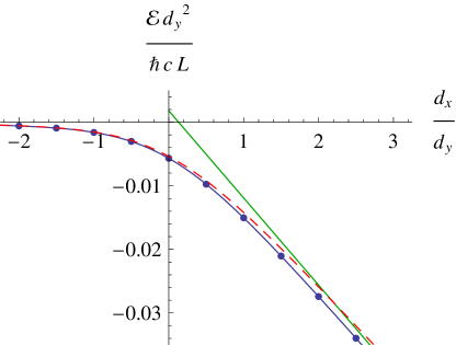
Figure 2: Electromagnetic Casimir interaction energy per unit length for overlapping planes as a function of horizontal displacement, in units of the vertical separation $d_{y}$. Circles are obtained from the exact calculation in parabolic cylinder coordinates. The solid line connecting them is a rational function fit to guide the eye. The dashed line gives the analytic formula obtained by considering only the first reflection, while the solid straight line gives the standard parallel plane result for the overlap area, plus edge corrections.

The calculation for a half-plane opposite an infinite plane proceeds analogously to the case of two planes, and has been done in detail in Refs. parabolic ; wedge . In Fig. 3 we show the coefficient $c(\theta)$ using both the exact numerical calculation in the parabolic cylinder basis parabolic and the approximation to two reflections in the wedge basis wedge , which is

$$\frac{{\cal E}}{\hbar cL}=-\frac{1}{16\pi^{2}d_{y}^{2}}\sec\theta-\frac{1}{256\pi^{3}d_{y}^{2}}\left(\frac{4}{3}+\csc^{3}\theta\sec\theta(2\theta-\sin 2\theta)\right)+\cdots\,,$$ (16)

where the dots indicate corrections from higher reflections (three reflections or more).

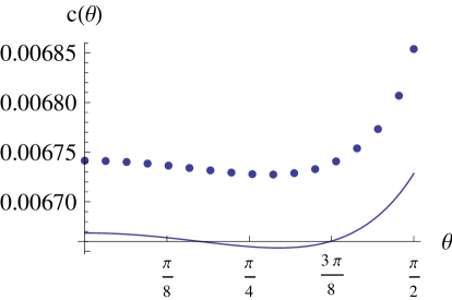
Figure 3: The orientation dependence $c(\theta)$ for the electromagnetic Casimir energy of a half-plane opposite a plane, as a function of the tilt angle $\theta$. Circles are obtained from the exact calculation in parabolic cylinder coordinates, while the solid line is obtained from the analytic expansion through two reflections, Eq. (16).

The comparison of the exact numerical calculation in the parabolic cylinder basis to the reflection expansion in the wedge basis shows both the strengths and weaknesses of this approximation. The expansion to two reflections for the energy of a tilted half-plane opposite a plane captures the orientation dependence $c(\theta)$ well. The variation in this quantity is small because of the near-cancellation of the Dirichlet and Neumann contributions. However, the relative error in the edge correction, that is, the error in the derivative of $c(\theta)$ as $\theta\to\pi/2$, is large because while the neglected contribution from the higher reflections is small, it varies rapidly as the planes become parallel. For $\theta=\pi/2$, the reflection expansion to order $n$ gives the parallel-plane result with $\zeta(4)$ truncated to the first $n$ terms in its series representation, but this error decreases as the angle deviates from $\pi/2$. This behavior can be anticipated from a geometric optics point of view, since as the planes become nonparallel, higher-order reflections must propagate further as they reflect between the planes. The analogous problem arises in extracting the edge correction from the overlapping planes calculation, since again the asymptotic result as $d_{x}\to\infty$ captures only the leading term in the zeta-function series.

Thermal Corrections

We can also apply these results to find the free energy in a system at temperature $T$. Then the integral over $\kappa$ is replaced by a sum over Matsubara frequencies $\kappa_{n}=2\pi nT/\hbar c$, where $n=0,1,2,\ldots$ and the $n=0$ contribution is counted with a weight of $1/2$. Again, we keep only the first reflection. For the case of a half-plane opposite a plane, we obtain the free energy for each polarization

$$\frac{{\cal F}^{D/N}}{k_{B}TL}=-\frac{1}{2\pi}{\sum_{\kappa_{n}\geq 0}}^{\prime}\int dk_{x}dk_{z}\ \frac{1}{4\pi}e^{-2d\sqrt{\kappa_{n}^{2}+k_{x}^{2}+k_{z}^{2}}}\frac{1}{\sqrt{\kappa_{n}^{2}+k_{x}^{2}+k_{z}^{2}}}\left(\pm\frac{\sqrt{\kappa_{n}^{2}+k_{z}^{2}}}{\sqrt{\kappa_{n}^{2}+k_{x}^{2}+k_{z}^{2}}}+\frac{1}{\cos\theta}\right)+\cdots\,,$$ (17)

where the dots represent higher reflections. The first term in parentheses cancels in the sum over polarizations, giving for electromagnetism

$$\frac{{\cal F}{{}^{EM}}}{\hbar cL}=-\frac{1}{32\pi^{2}}\frac{1}{\cos\theta}\frac{1}{\lambda_{T}d}\coth\frac{d}{\lambda_{T}}=-\frac{1}{32\pi^{2}d^{2}}\frac{1}{\cos\theta}\left[1+\frac{1}{3}\left(\frac{d}{\lambda_{T}}\right)^{2}-\frac{1}{45}\left(\frac{d}{\lambda_{T}}\right)^{4}+{\mathcal{O}\left(\frac{{d}^{6}}{\lambda_{T}^{6}}\right)}\right]+\cdots\,,$$ (18)

where $\lambda_{T}=\hbar c/(2\pi k_{B}T)$ is the thermal wavelength. The leading correction at small temperature is proportional to $T^{2}$, but this term is independent of distance and thus does not contribute to the force, for which the leading correction starts at order $T^{4}$. We note that in the case of a scalar field with either Dirichlet or Neumann boundary conditions, however, the first term in parentheses in Eq. (17) yields the contribution

$$\frac{\mathcal{F}{{}^{\pm}}}{\hbar cL}=\mp\frac{1}{16\pi^{3}}\frac{1}{\lambda_{T}d}\left[1+\frac{d}{\lambda_{T}}\int_{1}^{\infty}dt\,\frac{1}{t}{\rm\,csch}^{2}\left(\frac{d}{\lambda_{T}}t\right)E(1-t^{2})\right]\,,$$ (19)

where $E(x)$ is the elliptic function. This expression shows nonanalytic behavior as $T\to 0$ proportional to $T^{3}\ln T$, similar to what was observed in Ref. Gies .

References

- (1) H. B. G. Casimir, Proc. K. Ned. Akad. Wet. 51, 793 (1948).
- (2) T. Emig, N. Graham, R. L. Jaffe, and M. Kardar, Phys. Rev. Lett. 99, 170403 (2007); Phys. Rev. D 77, 025005 (2008).
- (3) S. J. Rahi, T. Emig, N. Graham, R. L. Jaffe, and M. Kardar, Phys. Rev. D 80, 085021 (2009).
- (4) N. Graham, A. Shpunt, T. Emig, S. J. Rahi, R. L. Jaffe, and M. Kardar, Phys. Rev. D 81, 061701(R) (2010).
- (5) M. F. Maghrebi, S. J. Rahi, T. Emig, N. Graham, R. L. Jaffe, and M. Kardar, arXiv:1010.3223.
- (6) M. F. Maghrebi, arXiv:1012.1060.
- (7) F. Khoshnoud, private communication.
- (8) H. Gies and K. Klingmuller, Phys. Rev. Lett. 97, 220405 (2006); A. Weber and H. Gies, Phys. Rev. D 80, 065033 (2009).
- (9) D. Kabat, D. Karabali, and V. P. Nair, Phys. Rev. D 82, 025014 (2010).
- (10) A. Scardicchio and R. Jaffe, Nucl. Phys. B 704, 552 (2005); Nucl. Phys. B 743, 249 (2006).
- (11) B. V. Derjaguin, I. I. Abrikosova, and E. M. Lifshitz, Q. Rev. Chem. Soc. 10, 295 (1956).
- (12) G. J. Maclay, Phys. Rev. A 82, 032106 (2010).
- (13) M. F. Maghrebi, R. Abravanel, and R. L. Jaffe, to be published.