1 INTRODUCTION

ALPHA, under construction at IU CEEM, is a 20-m electron storage ring. [1] The project calls for storing a tiny synchrotron-radiation-damped bunch to be extended to about 40 ns with uniform longitudinal distribution. RF barriers should be the best candidate for bunch lengthening. Unfortunately, this ring is only 66.6 ns in length, and the widths of the barriers must be of the order of 10 ns or less. The risetime of the barrier voltage will therefore be a few ns, or the rf generating the barrier voltage will be in the frequency range of a few hundred MHz. Ferrite is very lossy at such high frequencies and is therefore unsuitable for the job. Even if another material could be substituted, the barriers of such narrow widths would require very high rf peak voltage; the rf system would be very costly.

Another way to achieve bunch lengthening is to perform phase modulation of the rf wave so as to produce a large chaotic region at the center of the rf bucket, but bounded by well-behaved tori. The beam at the bucket center will be blown up to the much larger chaotic region. If true chaoticity is achieved, the particle distribution will be uniform. Such an idea has been demonstrated experimentally at the IUCF Cooler ring in 1997, [2] where a double-rf system was used and the diffusion was found rather sensitive to the phase difference $\Delta\phi_{0}$ between the two rf waves. In this paper, the modulation method is further investigated by first determining the choice of $\Delta\phi_{0}$, and next analyzing the condition and stability of the localized chaotic region.

2 THE MODEL

The model to be studied is described by the Hamiltonian $H=H_{0}+H_{1}$, where [3]

$$H_{0}\!=\frac{1}{2}\nu_{s}\delta^{2}\!+\!\nu_{s}\left\{1\!-\!\cos\phi\!-\!\frac{r}{h}\big{[}1\!-\!\cos(h\phi\!+\!\Delta\phi_{0})\big{]}\right\}\!,$$

$$H_{1}=a\delta\nu_{s}\sin(\nu_{m}\theta+\eta).$$ (1)

Here $r$ is the ratio of the two rf voltages, $h$ is the ratio of the two rf harmonics, $\nu_{s}$ is the small-amplitude synchrotron tune in the absence of the second rf, $\nu_{m}$ is the phase modulation tune, $\eta$ is the modulation phase, $a$ is the modulation amplitude, $\phi$ is the rf phase, $\delta$ is the canonical momentum offset, and $\theta$ advances by $2\pi$ per revolution turn. This model entails a number of parameters. In this paper, however, we restrict ourselves to the special case of $r=1/2$, $h=2$, $\nu_{m}/\nu_{s}=2$, and $\eta=0$, thus leaving behind only the phase offset $\Delta\phi_{0}$ and the modulation amplitude $a$.

2.1 Choice of $\Delta\phi_{0}$

The action at the bottom of an rf potential well $V(\phi)$ is zero and so are the resonance strengths generated by phase modulation (see Fig. 4 below). Since the bunch will be tiny, it will be difficult to be driven into parametric resonances if it sits at the bottom of the rf potential. This explains why a two-rf system is necessary. The phase difference $\Delta\phi_{0}$ between the two rf’s shifts the potential-well bottom away from the center of the longitudinal phase space, where the tiny bunch is located. The action at the bunch is now finite. Thus the farther the potential-well bottom is shifted, the larger the resonant strengths.

To generate a large region of chaoticity, the eventual modulation amplitude $a$ will be large. However, a perturbative approach is taken in the analysis so as to get a ball-park understanding of the mechanism. For the unperturbed Hamiltonian, the position of the potential-well bottom $\phi_{0}$ is given by $V^{\prime}(\phi_{0})/\nu_{s}=\sin\phi_{0}-r\sin(h\phi_{0}+\Delta\phi_{0})=0,$ and is at a maximum when $V^{\prime\prime}(\phi_{0})=0$. This leads to the solution $\phi_{0}=\pm\sin^{-1}r$. The corresponding phase difference between the two rf’s is therefore (see Fig. 1)

$$\Delta\phi_{0}=\frac{\pi}{2}-h\sin^{-1}r.$$ (2)

When $h\!=\!1/r\!=\!2$, the largest offset of well bottom is $\phi_{0}\!=\!\pm 30^{\circ}$ and the corresponding phase difference between the two rf’s is $\Delta\phi_{0}=\pm 30^{\circ}$.

Figure 1: Offset of potential-well bottom $\phi_{0}$ as a function of rf phase difference $\Delta\phi_{0}$ at $h=1/r=2$.

Simulations show that diffusion of a tiny bunch at the phase-space center is possible when $20^{\circ}\lesssim|\Delta\phi_{0}|\lesssim 50^{\circ}$. In below, we first study the case of $\Delta\phi_{0}=30^{\circ}$, and attempt another value later.

2.2 Synchrotron Tune and Resonance Strengths

For the unperturbed Hamiltonian, the action and angle of an oscillatory orbit are given by

$$J=\frac{1}{2\pi}\oint\delta(\phi)d\phi,~{}~{}~{}\psi=\frac{Q_{s}}{\nu_{s}}\int_{\phi_{1}}^{\phi}\frac{d\phi^{\prime}}{\delta(\phi^{\prime})},$$ (3)

where $\phi_{1}$ is smaller end of the phase excursion. When $\phi$ reaches the larger end of the phase excursion $\phi=\phi_{2}$ while $\psi$ advances by $\pi$, the synchrotron tune $Q_{s}$ of the oscillatory torus can be extracted, and is depicted in Fig. 3, where the asymmetric rf potential is also plotted in dot-dashes.

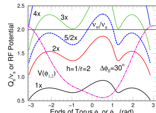
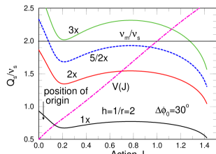
Figure 2: (color) Synchrotron tune $Q_{s}/\nu_{s}$ versus oscillating torus smaller end $\phi_{1}$ or larger end $\phi_{2}$, with $h\!=\!1/r\!=\!2$ and $\Delta\phi_{0}\!=\!30^{\circ}$. Some multiples are also plotted to illustrate the possible parametric resonances driven the phase modulation tune $\nu_{m}/\nu_{s}\!=\!2$ (horizontal line.) The asymmetric rf potential is shown in dot-dashes.

Figure 3: (color) Synchrotron tune $Q_{s}/\nu_{s}$ and its multiples as functions of action $J$, with $h=1/r=2$ and $\Delta\phi=30^{\circ}$. The rf potential $V(J)$ is shown in dot-dashes.

With the modulation tune $\nu_{m}/\nu_{s}\!=\!2$ (horizontal line), we see that the tiny bunch at the phase-space center will be driven into 3:1 and 5:2 resonances. The synchrotron tune can also be computed as a function of the action $J$, and this is depicted in Fig. 3. It is important to point out that we require the synchrotron tune to be large at the central part than the edges of the phase space, because we wish to have a central chaotic region bounded by well-behaved tori.

To express the perturbative Hamiltonian $H_{1}$ of Eq. (1) in terms of action-angle variables, the reduced momentum offset $\delta$ is expanded into Fourier series,

$$\delta\!=\!\sum_{n=-\infty}^{\infty}\!g_{n}(J)e^{in\psi},~{}~{}~{}g_{n}(J)\!=\!\frac{1}{2\pi}\!\int_{-\pi}^{\pi}\delta e^{-in\psi}d\psi.$$ (4)

Keeping only the first-order perturbative terms, the Hamiltonian can now be expressed as

$$H\!= H_{0}(J)+a\nu_{s}\bigg{\{}\!\sum_{n>0}|g_{n}(J)|\Big{[}\sin(\nu_{m}\theta\!+\!\eta\!+\!\chi_{n}\!+\!n\psi)~{}~{}~{}~{}~{}~{}$$

$$\!\!\!\!+\sin(\nu_{m}\theta\!+\!\eta\!+\!\chi_{n}\!-\!n\psi)\Big{]}\!+g_{0}(J)\sin(\nu_{m}\theta\!+\!\eta)\!\bigg{\}},\!\!\!\!\!$$ (5)

with $\chi_{n}$ the phase of $g_{n}$, showing all the first-order parametric resonances. The resonance strength function $|g_{n}|$ is a measure of its ability to drive the $n\!:\!1$ parametric resonance, and is depicted in Fig. 4 for $n\!=\!1$ to 4. Note that all the strength functions vanish at $J=0$, which is the reason why we need to shift the potential-well bottom away from the center of the phase space. Because of the asymmetry of $\delta(\phi)$, $g_{n}(J)$ no longer vanishes when $n$ is even, implying that both 2:1 and 3:1 resonances can be excited depending on the choice of the modulation tune $\nu_{m}$.

.

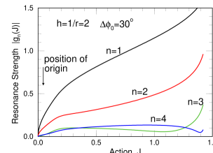
Figure 4: (color) Resonance strengths $|g_{n}(J)|$ as functions of the action $J$ for $n\!:\!1$ parametric resonances, with $n\!\leq\!4$, $h\!=\!1/r\!=\!2$.

3 SIMULATIONS WITH $\Delta\phi_{0}=30^{\circ}$

Simulation is performed by tracking each macro-particle from the $k$-th turn to the $(k\!+\!1)$-th turn according to the Hamiltonian of Eq. (1):

$$\!\!\!\phi_{k+1} \!=\!\phi_{k}\!+\!2\pi\nu_{s}\big{[}\delta_{k}\!+\!a\sin(2\pi k\nu_{m})\big{]},$$

$$\!\!\!\delta_{k+1} \!=\!\delta_{k}\!-\!2\pi\nu_{s}\big{[}\sin\phi_{k+1}\!-\!r\sin(h\phi_{k+1}+\Delta\phi_{0})\big{]},$$ (6)

where the assumption of slowly varying particle position within a turn has been applied. The modulation period has been chosen to be exactly 515 turns with $\nu_{m}/\nu_{s}=2$. The modulation phase has been taken to be $\eta=0$. Other values of $\eta$ will lead to different rotated stroboscopic views of the tracking results. However, all the conclusions on diffusion and beam enlargement will not be affected.

We first study the structure of the phase space at modulation amplitude $a=8^{\circ}$ and $\Delta\phi_{0}=30^{\circ}$, as depicted in Fig. 5.

Figure 5: Structure of phase space at $a=8^{\circ}$ and $\Delta\phi_{0}=30^{\circ}$.

This is the cumulative stroboscopic modulation-period views in half million turns. The central stable region is bounded by the 5:2 resonance. After that we see the remnant of the 8:3 resonance which merges partially with the 3:1 resonance. Then comes the 25:8 resonance and the well-behaved tori. In order for the bunch, initially at the phase-space center, to be enlarged via diffusion, we require the 5:2 resonance to collapse and the central stable region to shrink so that the bunch is inside the chaotic region initially. This occurs when the modulation amplitude increases to $a=46^{\circ}$.

Next a Gaussian distributed bunch of rms spread $\sigma_{\phi}=0.001$ rad consisting of 10000 macro-particles at the center of the longitudinal phase space is tracked. The particle distribution with modulation amplitude $a=58^{\circ}$ is shown in Fig. 6 at the last modulation period in 1.2 million turns. Essentially, the tiny bunch at the phase-space center is driven into the thick stochastic layers surrounding the separatrices of the 3:1 resonance.

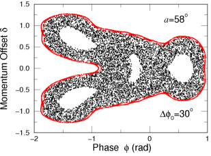
Figure 6: (color) Black: Diffusion of a tiny Gaussian bunch of rms spread $\sigma_{\phi}=0.001$ rad at phase-space center at the last modulation period in 1.2 million turns. Modulation amplitude is $a=58^{\circ}$. Red: Stroboscopic plot of one particle initially at $\phi=0.94$ rad and $\delta=0$ at every modulation period.

The thick stochastic layers, on the other hand, come from the overlapping of the 5:2, 8:3, and possibly many other higher-order resonances, which are not included in the first order perturbation of the modulation presented in Eq. (5). The distribution appears to be uniform except for the four big empty space, where the four stable fixed points of the 3:1 resonance are located. The rms beam size is computed turn by turn and is depicted in Fig. 7.

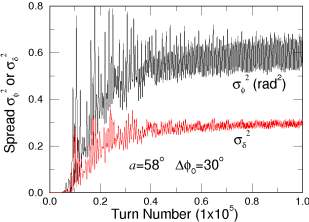
Figure 7: (color) Longitudinal bunch size versus turn number at $a=58^{\circ}$ and $\Delta\phi_{0}=30^{\circ}$ as diffusion develops.

We see that the rms-bunch-size squared, $\sigma_{\phi}^{2}$ or $\sigma_{\delta}^{2}$, grows linearly with turn number, signaling that the bunch enlargement is indeed a diffusion process. The growth levels off after about $1\times 10^{5}$ to $2\times 10^{5}$ turns. The rms phase and momentum spreads increase to $\sigma_{\phi}=0.81\pm 0.03$ rad and $\sigma_{\delta}=0.57\pm 0.01$, respectively.

We next continue the tracking by doubling the number of turns; the distribution remains bounded and the pattern does not change. We also track a particle initially at $\phi\!=\!0.94$ rad and $\delta\!=\!0$ for $1\!\times\!10^{5}$ turns. Its positions at every modulation period are shown as red dots in Fig. 6. These red dots constitute a well-behaved chain of islands, confirming that the diffused bunch will be well-bounded.

3.1 Variation of Modulation Amplitude

When the modulation amplitude is varied from $a=46^{\circ}$ to $70^{\circ}$, there is not much difference in the shape of the final diffused bunch distribution. The only significant change is the gradual left-shifting of the chaotic pattern in Fig. 6, which is a consequence of the detuning of the synchrotron tune $Q_{s}$ as the modulation amplitude $a$ increases. The diffused rms phase and momentum spreads are still roughly at $\sigma_{\phi}\approx 0.8$ rad and $\sigma_{\delta}\approx 0.58$, respectively, as depicted in Fig. 8.

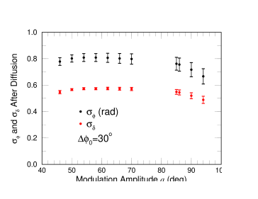
Figure 8: (color) Bunch spreads after diffusion at various modulation amplitudes with $\Delta\phi_{0}=30^{\circ}$.

When the modulation strength is increased past $a=70^{\circ}$, suddenly no diffusion is observed independent of how long the simulations are performed. This turns out to be the moment when the rightmost empty region in Fig. 6 has been left-shifted to include the phase-space origin. The bunch is now inside the rightmost island of the 3:1 resonance making small tori around the stable fixed points of the 3:1 resonance.

The diffusion of the bunch does return when the modulation strength increases up to $a\geq 85^{\circ}$. Now the three outside islands of the 3:1 resonance are completely filled up by higher-order resonances so that the tiny bunch initially at the phase-space center can diffuse outward again.

As the modulation amplitude continues to increase, the phase-space structure tends to contract and shift further to the left. As $a>94^{\circ}$, the bunch original position moves out of the chaotic region and no diffusion occurs. A typical phase-space pattern at $a=104^{\circ}$ is shown in Fig. 9.

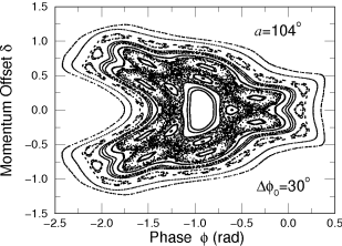
Figure 9: Stroboscopic plot of phase-space structure at $a=104^{\circ}$ and $\Delta\phi=30^{\circ}$, showing that the bunch original position lies on a well-behaved torus completely outside the chaotic region.

As $a$ increases past $110^{\circ}$, beam loss occurs.

4 SIMULATIONS WITH $\Delta\phi_{0}=45^{\circ}$

Figures 3 and 3 shows that the approximate intercepts of horizontal line $\nu_{m}/\nu_{s}=2$ with the $3\times Q_{s}/\nu_{s}$ curve are far away from the initial location of the particle bunch. In other words, the bunch is initially far from the unstable fixed points of the 3:1 resonance. This limits the bunch from falling inside the stochastic layers surrounding the separatrices unless the modulation amplitude is sufficiently large. Figure 4 shows that the strength function of the 3:1 resonance is much smaller than that of the 2:1 resonance and as a result very large modulation amplitude has to be employed. All these reasons educe us to a deviation from the maximum potential-well-bottom offset. Here, we try the rf phase difference $\Delta\phi_{0}\!=\!45^{\circ}$, which leads to a well-bottom offset of $\phi_{0}\!=\!29.12^{\circ}$, which is only 3% less than the maximum value of $30^{\circ}$. This explains why the range of $\Delta\phi_{0}$ that can produce bunch lengthening is not too narrow.

Corresponding to Fig. 3, the synchrotron tune as a function of action for $\Delta\phi_{0}=45^{\circ}$ is shown in Fig. 10.

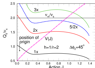
Figure 10: (color) Synchrotron tune $Q_{s}/\nu_{s}$ as a function of action $J$, with $h=1/r=2$ and $\Delta\phi_{0}=45^{\circ}$. $2\times$, $5/2\times$, and $3\!\times\!Q_{s}/\nu_{s}$ are also plotted to illustrate the possible parametric resonances driven at the phase modulation frequency $\nu_{m}/\nu_{s}=2$. The rf potential $V(J)$ is shown in dot-dashes.

Observe that where the horizontal line $\nu_{m}/\nu_{s}\!=\!2$ cuts the $2\times Q_{s}/\nu_{s}$ curve is extremely close to $J\!=\!0.053$, the initial location of bunch, implying close proximity of the bunch from an unstable fixed point of the 2:1 resonance. We should expect diffusion to occur at relatively smaller modulation amplitudes. The resonance strength functions for $\Delta\phi_{0}\!=\!45^{\circ}$ do not differ much in value from those for $\Delta\phi_{0}\!=\!30^{\circ}$ in Fig. 4.

The phase-space structure when $\Delta\phi_{0}=45^{\circ}$ and $a=7^{\circ}$ is illustrated in Fig. 11.

Figure 11: Structure of phase space at $a=7^{\circ}$ and $\Delta\phi_{0}=45^{\circ}$.

We first notice that the phase-space center is very close to the 2:1 resonance as speculated. However, the tiny bunch there can only spread out inside the thin stochastic layers of the 2:1 resonance, and cannot reach the larger chaotic region between the island chains of the 8:5 and 7:3 resonances. The bunch can diffuse into this region only when the chains of higher-order islands enclosing the 2:1 resonance collapse. This happens when $a\approx 9^{\circ}$, which explains the rapid jump of simulated bunch-spread results from $a=8^{\circ}$ to $10^{\circ}$ in Fig. 12.

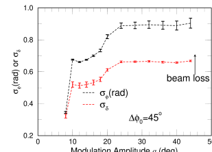
Figure 12: (color) Bunch spreads at various modulation amplitudes with $\Delta\phi_{0}=45^{\circ}$.

A typical diffused bunch distribution is shown in Fig. 13, corresponding to modulation amplitude $a\!=\!28^{\circ}$ at the last modulation period after roughly 0.5 million turns. Compared with Fig. 6 at $\Delta\phi_{0}\!=\!30^{\circ}$, it is evident that the chaotic area is much larger and the empty space inside is very much smaller. It also looks much more rectangular, and will provide a more uniform linear density. At the same time the modulation amplitude $a=28^{\circ}$ is about one-half smaller. The red dots are stroboscopic loci of one particle initially located at $\phi\!=\!1.46$ rad and $\delta\!=\!0$. These loci provide a well-behaved torus bounding the diffused bunch.

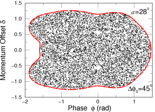
Figure 13: (color) Black: Bunch distribution at the last modulation period after $\sim\!0.5$ million turns with $a\!=\!28^{\circ}$ and $\Delta\phi\!=\!45^{\circ}$. Red: Stroboscopic plot of one particle initially at $\phi=0.94$ rad and $\delta=0$ at every modulation period.

The rms phase and momentum-offset spreads shown in Fig. 14 reveal linear growths of $\sigma_{\phi}^{2}$ and $\sigma_{\delta}^{2}$, demonstrating the occurrence of diffusion. Compared with Fig. 7 at $\Delta\phi_{0}\!=\!30^{\circ}$, equilibrium is reached much earlier. This is understandable because the bunch initially is much closer to the separatrices of the 2:1 resonance, and obviously, will take less time to diffuse.

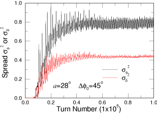
Figure 14: (color) Longitudinal bunch-size squared turn by turn at $a\!=\!28^{\circ}$ and $\Delta\phi_{0}\!=\!45^{\circ}$ as diffusion develops.

As illustrated in Fig. 12, there is another jump of beam size around $a\approx 20^{\circ}$. This can be explained by the hump of the synchrotron frequency around action $J\approx 0.7$ in Fig. 10. As a result, there are two sets of 8:3 resonances, one going out and one coming in as the modulation amplitude $a$ increases. The one going out has already broken at $a\approx 7$. The incoming set encircling the chaotic region starts collapsing around $a=20^{\circ}$, and the chaotic region is increased after that. This is illustrated in Fig. 15.

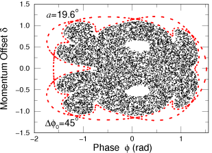
Figure 15: (color) Black: Bunch distribution at the last modulation period after $\sim\!0.5$ million turns at $a=9.8^{\circ}$ and $\Delta\phi_{0}=45^{\circ}$. Red: A chain of 8 islands forming a boundary for the diffused region. At an increase to $a\approx 20^{\circ}$, the separatrices of the island chain collapse, and the islands join the region of diffusion.

5 CONCLUSION

We have devised a method of phase modulation of the rf wave to create a large chaotic region in the central longitudinal phase space bounded by well-behaved tori. To accomplish this, we require (1) large modulation amplitude so that higher-order parametric resonances collapse to form a large chaotic area, and (2) the initial position of the tiny bunch inside this chaotic region. Since the bunch is initially located at the phase-space center, we must offset the relative phase of the two-rf system so that the potential-well bottom is shifted away from the phase-space center. The maximum well-bottom offset and the corresponding relative phase difference between the two rf’s are computed.

References

- [1] J. Doskow, etal, “The ALPHA Project at IU CEEM,” IPAC’10, 268.
- [2] D. Jeon, etal, “A Mechanism of Anomalous Diffusion in Particle Beams,” Phys. Rev. Lett. 80, (1998) 2314. C.M. Chu, etal, “Effects of Overlapping Parametric Resonances on the Particle Diffusion Process,” Phy. Ref. E60, (1999) 6051. K.Y. Ng, “Particle Diffusion in Overlapping Resonances,” Advanced IFCA Workshop on Beam Dynamics Issues for Factories, Frascati, Oct. 20-25, 1997 (Fermilab-Conf-98/001).
- [3] J.Y. Liu, etal, “Analytic Solution of Particle Motion in a Double RF System,” Particle Accelerators 49, (1995) 221.