Distributed Throughput-optimal Scheduling in
Ad Hoc Wireless Networks

Abstract

In this paper, we propose a distributed throughput-optimal ad hoc wireless network scheduling algorithm, which is motivated by the celebrated simplex algorithm for solving linear programming (LP) problems. The scheduler stores a sparse set of basic schedules, and chooses the max-weight basic schedule for transmission in each time slot. At the same time, the scheduler tries to update the set of basic schedules by searching for a new basic schedule in a throughput increasing direction. We show that both of the above procedures can be achieved in a distributed manner. Specifically, we propose an average consensus based link contending algorithm to implement the distributed max weight scheduling. Further, we show that the basic schedule update can be implemented using CSMA mechanisms, which is similar to the one proposed by Jiang et al. [1]. Compared to the optimal distributed scheduler in [1], where schedules change in a random walk fashion, our algorithm has a better delay performance by achieving faster schedule transitions in the steady state. The performance of the algorithm is finally confirmed by simulation results.

I Introduction

Scheduling in ad hoc wireless networks is, in general, an NP-complete problem. In order to achieve throughput optimality, one either needs to solve a problem with exponential complexity in each time slot (e.g., the max-weight scheduler in [2]), or by amortizing the complexity among an exponential number of time slots (e.g., the random “pick-and-compare” scheduler in [3]), so that the number of operations required in each time slot is constant, at the expense of large (exponential in the network size) queue lengths in the worst case [4].

In addition, the requirement that the scheduler be implemented in a distributed manner makes the scheduling problem more difficult to solve. In the literature, distributed scheduling algorithms are often designed to be sub-optimal (e.g., the greedy schedulers in [5], [6], [7]), so that minimal coordinations among links are needed during scheduling. Recently, Jiang et al. [1] showed a surprising result that, distributed throughput-optimal scheduling can be achieved by cleverly adjusting the CSMA contending parameters, which is based on the theory of Markov Chain Monte Carlo (MCMC). A throughput optimal scheduler is one that can achieve the rate stability for any arrival process whose average rate can be stabilized by some scheduler. This result has spurred interest among researchers in searching for other distributed throughput-optimal scheduling algorithms [8], [9], [10]. However, since these current scheduling algorithms are all based on the MCMC, they may suffer from large delays, even if they could begin in steady state (i.e., with optimal CSMA parameters chosen initially). This is due to the random walk behavior of the embedded time reversible Markov chain, which requires a long time, in general, for the schedule to change significantly. To illustrate this point, consider the star-shaped interference graph in Fig. 1 (a), where each node represents a link in the wireless network, and each edge represents a transmission conflict. Thus, the transmission schedules must be independent sets of the graph, e.g., $\{0\}$, and $\{1,2,3,4,5,6\}$. Due to the star-shaped topology, these two independent sets can also be viewed as the two “modes” of this network. Now, the distributed CSMA scheduling implies that the scheduled independent sets form a random walk on the family of independent sets, where transitions are only allowed between independent sets which differ by one link. For example, the schedule can change from $\{1\}$ to $\{1,2\}$, but not from $\{1\}$ to $\{0\}$, since that requires two simultaneous changes: shutting down link 1 and activating link 0. Suppose the current schedule is at mode $\{1,2,3,4,5,6\}$. In order to switch to the other mode $\{0\}$, all of the links $\{1,2,3,4,5,6\}$ need to stop transmission first, so that link 0 is able to contend for transmission. Intuitively, this takes a long time, in particular, if the other links are unwilling to stop transmission, due to their own traffic demands. Thus, the distributed CSMA scheduling may incur a large delay by spending a long time in each mode before transition, since the random walk based design requires the scheduler to go through the intermediate (sub-optimal) schedules before switching to another mode, which happens with low probability. For more details about the steady state delay, please see the queueing simulation result in Fig. 3, which is explained in detail in Section IV.

(a)	(b)

Figure 1: (a) is a star-shaped interference graph of 7 links, and (b) is a ring-shaped interference graph of 6 links.

Realizing the limitations of these distributed CSMA scheduling algorithms, we try to improve the delay performance by avoiding the random-walk based transitions between schedules. Instead of allocating positive probabilities to all the schedules, as required by MCMC, we require that the scheduler choose the transmitting schedules among a sparse set of explicitly enumerated “modes” (basic schedules), so that the schedule transitions are faster, since there is no need for the scheduler to enter the sub-optimal “transition modes”. Further, since the number of basic schedules is small, optimal scheduling, from among these schedules, can be achieved efficiently in a distributed fashion. This is done by solving a simple max-weight independent set problem, which can be achieved by a certain consensus algorithm.

The existence of such a sparse optimal solution is guaranteed by the well-known Carathéodory theorem [12], which states that, at most $n+1$ schedules are needed to achieve the optimal scheduling in a network with $n$ links. Further, such a solution can be efficiently computed by the celebrated simplex algorithm [11], which can be viewed as a steepest descent algorithm along the edges of the feasible region (a polytope for LP). Inspired by the simplex algorithm, we propose a distributed algorithm to search for the optimal basic schedules, which can be implemented using distributed CSMA mechanisms similar to [1]. Thus, by combining the consensus based scheduling and CSMA based basic schedule updates, we show that throughput optimal scheduling can be achieved in a distributed fashion. Finally, the delay improvement is verified in the simulation section.

The organization of the rest of the paper is as follows: In Section II we introduce the system model, and in Section III we propose and analyze the scheduling algorithm. Section IV shows the simulation results, and finally Section V concludes this paper.

II System Model

In this section we introduce the system model, which is standard in the literature. We first introduce the network model.

II-A Network Model

We are interested in the scheduling problem at the MAC layer of a wireless network, where the topology of the network is described by an interference graph $\mathcal{G}_{I}=(\mathcal{V}_{I},\mathcal{E}_{I})$, where $\mathcal{V}_{I}$ is the set of $n$ links, and $\mathcal{E}_{I}$ is the set of pairwise interference constraints, i.e., link $i$ and link $j$ are not allowed to transmit together if $(i,j)\in\mathcal{E}_{I}$, due to the strong interference that one link causes upon the other. We assume a slotted time system, and in each time slot $t$, the scheduled transmitting links $\boldsymbol{\sigma}_{\text{sch}}(t)$ must form an independent set in $\mathcal{G}_{I}$. With an abuse of notation, we also denote $\boldsymbol{\sigma}_{\text{sch}}(t)$ as an $n\times 1$ vector, where $\sigma_{\text{sch},i}(t)=1$ if link $i$ belongs to the transmitting independent set, and $\sigma_{\text{sch},i}(t)=0$ otherwise.

The queueing dynamics of the network is as follows:

$$\boldsymbol{Q}(t)=\boldsymbol{Q}(0)+\boldsymbol{A}(t)-\boldsymbol{D}(t)$$ (1)

where $\boldsymbol{Q}(t)$ is the queue length vector at time slot $t$, and $\boldsymbol{A}(t)$ and $\boldsymbol{D}(t)$ are the number of cumulative arrived and departed packets during the first $t$ time slots, respectively. We assume that the packet arrival process is subject to the Strong Law of Large Numbers (SLLN), i.e., with probability 1 (w.p.1), we have $\lim_{t\rightarrow\infty}\boldsymbol{A}(t)/t=\boldsymbol{a}$ where $\boldsymbol{a}$ is the arrival rate vector. Further, we also assume that the number of arrived packets in each time slot is uniformly bounded by a large constant. Note that this assumption is quite mild, since the packet arrivals are allowed to be correlated both across time slots, and different links. Thus, our model is well suited in analyzing typical wireless networks, and can be readily generalized to multi-hop scenarios.

A basic requirement on the scheduler is the rate stability, i.e., for each link $i$, we have $\lim_{t\rightarrow\infty}D_{i}(t)/t=a_{i}$, w.p.1, so that an average throughput of $\boldsymbol{a}$ can be achieved by the scheduler. Thus, a throughput optimal scheduler should achieve rate stability for any $\boldsymbol{a}$ which can be stabilized by some scheduler. In the seminal paper [2], Tassiulas et al. showed that the optimal stability region is $\mathcal{A}={\bf Co}(\mathcal{M})$, where ${\bf Co}(\cdot)$ denotes the convex hull, and $\mathcal{M}$ is the family of all independent sets. Further, they propose the following optimal max-weight scheduling algorithm:

$$\boldsymbol{\sigma}_{\text{sch}}(t)=\arg\max_{\boldsymbol{\sigma}\in\mathcal{M}}\boldsymbol{\sigma}^{T}\boldsymbol{Q}(t)$$ (2)

However, such an algorithm requires solving an NP-complete problem in every time slot, and is very difficult to implement in a distributed manner. In the next subsection we introduce the recently developed throughput optimal distributed CSMA scheduling algorithm.

II-B Throughput Optimal Distributed Scheduling

Before introducing the distributed CSMA scheduling algorithm, we need to have an optimization interpretation of the scheduling problem. We can formulate the scheduling problem as the following feasibility problem:

$$\textsf{SCH: }\text{minimize}_{\boldsymbol{x}} 0$$ (3)

subject to $$M\boldsymbol{x}=\boldsymbol{a}$$ (5)

$$\boldsymbol{1}^{T}\boldsymbol{x}=1,\boldsymbol{x}\succeq\boldsymbol{0}$$

where $\boldsymbol{a}$ is the arrival rate vector, $M$ is the matrix whose columns are all the independent sets, and $\boldsymbol{x}$ is the scheduling variable, such that $x_{\boldsymbol{\sigma}}$ represents the asymptotic time fraction that independent set $\boldsymbol{\sigma}$ (which is a column of the matrix $M$) is chosen by the scheduler. Thus, $\boldsymbol{x}$ naturally lives in the simplex, as described by (5), and (5) is essentially the rate stability constraint.

Note that SCH has many solutions, due to the key structure in the highly under-determined system in (5) that, any subset of an independent set is also an independent set. Thus, based on a solution for any strictly feasible arrival rate vector $\boldsymbol{a}$, one can easily construct a set of feasible solutions. However, distributed implementation of any solution is a very challenging problem. In [1], Jiang et al. obtains a solution in the exponential family by transforming SCH into the following max-entropy problem ME:

$$\textsf{ME: }\text{maximize}_{\boldsymbol{x}} H(\boldsymbol{x})=-\sum_{\boldsymbol{\sigma}\in\mathcal{M}}x_{\boldsymbol{\sigma}}\log x_{\boldsymbol{\sigma}}$$

subject to $$(\ref{eqn_rate_constraint})\text{ and }(\ref{eqn_simplex_constraint})$$

It can be shown that the solution $\boldsymbol{x}^{\star}$ has the following form:

$$x_{\boldsymbol{\sigma}}^{\star}=\exp(\boldsymbol{\theta}^{\star T}\boldsymbol{\sigma}-A(\boldsymbol{\theta}^{\star}))$$ (6)

where $\boldsymbol{\theta}^{\star}$ corresponds to the Lagrange multiplier associated with the rate constraints in (5), and

$$A(\boldsymbol{\theta}^{\star})=\log\sum_{\boldsymbol{\sigma}\in\mathcal{M}}\exp(\boldsymbol{\theta}^{\star T}\boldsymbol{\sigma})$$ (7)

is the standard log-partition function. Following the literature of Gibbs sampling (an example of MCMC), it was shown in [1] that the optimal allocations $\boldsymbol{x}^{\star}$ can be implemented by a time-reversible Markov chain, using CSMA mechanisms. Further, the optimal parameters (Lagrange multipliers) $\boldsymbol{\theta}^{\star}$ can be obtained using a stochastic gradient algorithm. In below we describe a discrete-time version of the distributed scheduling algorithm, which is also closely related to the algorithm in [8].

Algorithm 1 CSMA($\boldsymbol{\theta}$)

  In each time slot $t$, do the following:

  Randomly generate an independent set $\boldsymbol{\sigma}(t)$ from a certain distribution, independently across time slots.

  for each $i\in\boldsymbol{\sigma}(t)$ do

     $p_{i}=\exp(\theta_{i})/(1+\exp(\theta_{i}))$;

     if  no neighbor of $i$ is in $\boldsymbol{\sigma}_{\text{csma}}(t-1)$ then

        

$$\sigma_{\text{csma},i}(t)=\left\{\begin{array}[]{ll}1&\textrm{ with probability }p_{i}\\ 0&\textrm{ else }\end{array}\right.$$

     end if

  end for

  Any other link $i$ not in $\boldsymbol{\sigma}(t)$ set $\sigma_{\text{csma},i}(t)=\sigma_{\text{csma},i}(t-1)$.

In the above algorithm, carrier sensing is used in two phases: 1) generation of the independent set $\boldsymbol{\sigma}(t)$ (according to certain protocol [8]) and 2) detection of whether there is a transmitting neighbor of a link $i\in\boldsymbol{\sigma}(t)$ at time slot $t-1$. Further, note that the key part of the algorithm, phase 2, is fully distributed, with no explicit message exchange among links. The following proposition shows that the above algorithm achieves the distribution in (6) asymptotically.

Proposition 1

$\boldsymbol{\sigma}_{\text{csma}}(t)$ in CSMA$(\boldsymbol{\theta}^{\star})$ form a time-reversible Markov chain, with the steady state distribution in the form of (6).

Proof:

The claim is proved by checking balance equations. The proof is essentially the same as the one in [8], which we omit due to space limitation. ∎

As discussed in Section I, however, the above scheduling algorithm suffers from long delay, due to the random walk behavior associated with the time-reversible Markov chain. In the following section we try to solve this problem by introducing the simplex scheduling algorithm.

III Simplex Scheduling

In this section we propose optimal distributed scheduling, which is based on the simplex algorithm. For a detailed description of the simplex algorithm for general LP problems, please see, for example, [11]. Since the simplex algorithm requires a feasible starting point, we next transform the problem SCH into a relaxed problem REL, where a feasible initial vertex is easy to obtain:

$$\textsf{REL: }\text{minimize}_{\boldsymbol{x},\gamma} \gamma$$ (8)

subject to $$M\boldsymbol{x}=(1-\gamma)\boldsymbol{a}$$ (10)

$$\boldsymbol{1}^{T}\boldsymbol{x}=1,\boldsymbol{x}\succeq\boldsymbol{0},0\leq\gamma\leq 1$$

In above, the relaxation variable $\gamma$ can be interpreted as the “throughput gap”, so that $\gamma^{\star}=0$ if and only if the arrival rate $\boldsymbol{a}$ can be stabilized by the scheduler. In order to illustrate the main ideas of the distributed scheduling algorithm, we first introduce a hypothesized centralized simplex algorithm to solve REL.

III-A Centralized Simplex Scheduling

The centralized simplex algorithm SIM is shown in Algorithm 2, which is essentially an application of the general simplex algorithm to the specific scheduling problem REL.

Algorithm 2 SIM

  Initialization: $B=I,\boldsymbol{x}_{B}^{\star}=\min({1\over\boldsymbol{1}^{T}\boldsymbol{a}},1)\boldsymbol{a},\gamma^{\star}=\max(1-{1\over\boldsymbol{1}^{T}\boldsymbol{a}},0)$.

  while $\gamma^{\star}>0$ do

     

1. Simplex Search: Compute the moving direction

   $$\boldsymbol{\sigma}_{\text{new}}=\arg\max_{\boldsymbol{\sigma}\in M}\boldsymbol{1}^{T}B^{-1}\boldsymbol{\sigma}\$$ (11)

2. Scheduling: Compute the new vertex $(\boldsymbol{x}_{B}^{\star},x_{\text{new}}^{\star})$ and the throughput gap $\gamma^{\star}$ by solving

   $$\textsf{MOV: }\min_{\boldsymbol{x}_{B},x_{\text{new}},\gamma} \gamma$$

   subject to $$B\boldsymbol{x}_{B}+\boldsymbol{\sigma}_{\text{new}}x_{\text{new}}=(1-\gamma)\boldsymbol{a}$$

   $$\boldsymbol{1}^{T}\boldsymbol{x}_{B}+x_{\text{new}}=1$$

   $$\boldsymbol{x}_{B}\succeq\boldsymbol{0},x_{\text{new}}\geq 0,0\leq\gamma\leq 1$$

3. Update: Let be $\boldsymbol{\sigma}$ be a column in $B$ such that $x^{\star}_{\boldsymbol{\sigma}}=0$. Replace $\boldsymbol{\sigma}$ with $\boldsymbol{\sigma}_{\text{new}}$, and relabel the variables.

  end while

  return  $(B,\boldsymbol{x}_{B}^{\star},\boldsymbol{\gamma}^{\star})$

The above simplex algorithm solves the problem REL by moving along adjacent vertices of the feasible region in a cost reducing direction. In order to understand its behavior, we first need to identify a vertex. According to the equality constraints in REL, a vertex (or a basic solution in the simplex algorithm terminology) $(\boldsymbol{x}_{B},\gamma)$ can be uniquely determined by a basis matrix as follows:

$$\left(\begin{matrix}B&\boldsymbol{a}\\ \boldsymbol{1}^{T}&0\end{matrix}\right)\left(\begin{matrix}\boldsymbol{x}_{B}\\ \gamma\end{matrix}\right)=\left(\begin{matrix}\boldsymbol{a}\\ 1\end{matrix}\right)$$ (12)

where $B$ is an $n\times n$ (invertible) sub-matrix of $M$, which represents $n$ independent sets, and $\boldsymbol{x}_{B}$ is an $n\times 1$ sub-vector of $\boldsymbol{x}$, which are the allocated time fractions of the independent sets in $B$. It is easy to verify that the initial vertex as specified in the initialization phase of SIM is feasible.

We next show that SIM successfully moves to an adjacent vertex following a cost reducing direction. An edge is represented by a new column vector $\boldsymbol{\sigma}\choose\boldsymbol{1}$, where $\boldsymbol{\sigma}$ is an independent set, and moving along the edge is equivalent to increasing the coefficient associated with $\boldsymbol{\sigma}\choose\boldsymbol{1}$, with the constraint that the equalities in REL still hold. Thus, the changes of the optimization variables must stay in the null space of the matrix $\left(\begin{matrix}M&\boldsymbol{a}\\ \boldsymbol{1}^{T}&0\end{matrix}\right)$, i.e., we increase the coefficient of $\boldsymbol{\sigma}\choose 1$ by a unit, the changes in the existing variables are

$$\left(\begin{matrix}B&\boldsymbol{a}\\ \boldsymbol{1}^{T}&0\end{matrix}\right)\left(\begin{matrix}\Delta\boldsymbol{x}_{B}\\ \Delta\gamma\end{matrix}\right)+\left(\begin{matrix}\boldsymbol{\sigma}\\ 1\end{matrix}\right)=\boldsymbol{0}$$ (13)

Using the block matrix inversion formula, we obtain the rate of change in the cost:

$$\Delta\gamma=(1-\gamma)(1-\boldsymbol{1}^{T}B^{-1}\boldsymbol{\sigma})$$ (14)

Thus, we need to find a proper independent set $\boldsymbol{\sigma}$, so that the cost change $\Delta\gamma\leq 0$. We next show that the $\boldsymbol{\sigma}^{\star}$ obtained in (11) is a proper cost-reducing direction.

Proposition 2

The cost change for the independent set $\boldsymbol{\sigma}^{\star}$ in (11) satisfies $\Delta\gamma\leq 0$, and the inequality is strict if $\gamma>0$.

Proof:

From (12) we have $\boldsymbol{x}_{B}=(1-\gamma)B^{-1}\boldsymbol{a}$. After multiplying both sides with $\boldsymbol{1}^{T}$ and noting that $\boldsymbol{1}^{T}\boldsymbol{x}_{B}=1$, we have

$$(1-\gamma)(\boldsymbol{1}^{T}B^{-1}\boldsymbol{a})=1$$ (15)

Noting that $\boldsymbol{a}\in{\bf Co}(\mathcal{M})$ and (11), we have

$$\boldsymbol{1}^{T}B^{-1}\boldsymbol{\sigma}^{\star}\geq\boldsymbol{1}^{T}B^{-1}\boldsymbol{a}$$ (16)

and therefore

$$\Delta\gamma = (1-\gamma)(1-\boldsymbol{1}^{T}B^{-1}\boldsymbol{\sigma}^{\star})$$

$$\leq (1-\gamma)(1-\boldsymbol{1}^{T}B^{-1}\boldsymbol{a})=-\gamma$$

from which the claim follows. ∎

Given the new direction specified by $\boldsymbol{\sigma}^{\star}$, according to the standard simplex algorithm, SIM then moves along the edge as specified by ${\boldsymbol{\sigma}^{\star}\choose 1}$, until it reaches a new vertex, where some coefficient of the independent set in $B$ first becomes zero. Then SIM replaces that column with $\boldsymbol{\sigma}^{\star}$, and relabel the variables if necessary. We next show that, this movement to a better vertex is achieved by solving the problem MOV.

Proposition 3

For the solution $(\boldsymbol{x}_{B}^{\star},x_{\text{new}}^{\star},\gamma^{\star})$ to the problem MOV, we have $x_{\text{new}}^{\star}>0$, and there is one column $\boldsymbol{\sigma}$ in $B$ such that $x^{\star}_{\boldsymbol{\sigma}}=0$.

Proof:

Due to space limitation, we only describe the intuition behind the proof. Suppose $x_{{\text{new}}}^{\star}=0$, then the solution to MOV is at the same vertex associated with the old matrix $B$, which contradicts the fact that $\boldsymbol{\sigma}_{\text{new}}$ is a cost-reducing direction, according to Proposition 2. The claim that some $\boldsymbol{\sigma}$ in $B$ has $x^{\star}_{\boldsymbol{\sigma}}=0$ follows from the fact that MOV has bounded optimum. ∎

Having shown that the centralized algorithm SIM is the same as the general simplex algorithm for LP problems, we have the following conclusion:

Theorem 1

If $\boldsymbol{a}\in{\bf Co}(\mathcal{M})$, SIM will return a solution $(B,\boldsymbol{x}_{B}^{\star},\gamma^{\star})$ such that $\gamma^{\star}=0$, and $(\boldsymbol{x}_{B}^{\star},\gamma^{\star})$ solves REL.

In the next subsection we show that this algorithm can be efficiently implemented in a distributed manner, using CSMA and average consensus algorithms.

III-B Distributed Simplex Scheduling

In this subsection we propose the distributed scheduling problem, and prove its throughput optimality, by showing that it is a distributed implementation of the centralized simplex scheduling algorithm in the last subsection. We first illustrate the full scheduling algorithm DIS-SCH in Algorithm 3.

Algorithm 3 DIS-SCH

  Initialization: Set the initial parameters as $B(0)=I$, $\boldsymbol{\theta}(0)=\boldsymbol{0}$, $\gamma(0)=1$, $\boldsymbol{\sigma}_{\text{csma}}(0)=\boldsymbol{0}$, and $\boldsymbol{\sigma}_{\text{new}}(0)=\boldsymbol{0}$.

  In each time slot $t$, do the following:

1. CSMA: update $\boldsymbol{\sigma}_{\text{csma}}(t)$ by running CSMA($\alpha\boldsymbol{\theta}(t)$), where $\alpha$ is a sufficiently large constant.

2. Scheduling: for each link $i$, compute

   $$\sigma_{\text{sch},i}(t)=\arg\max_{\boldsymbol{\sigma}\in B\cup\{\boldsymbol{\sigma}_{\text{new}}\}}w^{(i)}_{\boldsymbol{\sigma}}(t)$$ (17)

   Link $i$ transmits if $\sigma_{\text{sch},i}(t)=1$. In above, $w_{\boldsymbol{\sigma}}(t)=\boldsymbol{\theta}(t)^{T}\boldsymbol{\sigma}$ is the weight of independent set $\boldsymbol{\sigma}$, and $w^{(i)}_{\boldsymbol{\sigma}}(t)$ is link $i$’s local copy, which is updated by the consensus algorithm.

3. Consensus: update the parameters

   $$\boldsymbol{\theta}(t) = \boldsymbol{\theta}(t)+\epsilon(\boldsymbol{(}1-\gamma(t))\boldsymbol{a}(t)-\boldsymbol{\sigma}_{\text{sch}}(t))$$ (18)

   $$\gamma(t) = [\gamma(t)+\epsilon(\boldsymbol{\theta}(t)^{T}\boldsymbol{a}(t)-1)]_{[0,1]}$$ (19)

   $$\boldsymbol{a}(t) = \boldsymbol{A}(t)/t$$ (20)

   where $[\cdot]_{[0,1]}$ means projecting onto the interval $[0,1]$, and $\epsilon$ is a constant step size. Run an average consensus algorithm over the quantities $\{w_{\boldsymbol{\sigma}}(t)\}_{\boldsymbol{\sigma}\in B\cup\{\boldsymbol{\sigma}_{\text{new}}\}}$ and $\gamma(t)$.

4. Update: If certain convergence conditions are satisfied, replace the column in $B$ with the smallest weight by $\boldsymbol{\sigma}_{\text{new}}(t)$, and load the CSMA independent set by letting $\boldsymbol{\sigma}_{\text{new}}(t)=\boldsymbol{\sigma}_{\text{csma}}(t)$.

Overall DIS-SCH is very similar to SIM, with the following two important changes: 1) the simplex search phase in SIM is replaced with the CSMA phase, and that 2) the centralized moving procedure MOV is replaced with a simple max-weight scheduling in (17), which is then followed by parameter updates and average consensus algorithm. It may appear that (17) is similar to the max-weight scheduler in (2), with the difference that the queue lengths $\boldsymbol{Q}(t)$ are replaced by the “virtual queue lengths” $\boldsymbol{\theta}(t)$. However, the max-weight independent set in (17) is chosen from $n+1$ independent sets, instead of the family of all independent sets, which has exponential size. Thus, (17) can be solved efficiently (in linear time), whereas the max-weight scheduler in (2) is NP-complete, in general. In the following we elaborate on the change in Step 2, by showing that the scheduling and consensus phases in DIS-SCH is equivalent to solving the problem MOV.

Proposition 4

If there is no change in the matrix $B$, the parameters $\boldsymbol{\theta}$ updated in (18) will converge to the optimal dual variable for MOV, $\gamma$ will converge to the optimal cost $\gamma^{\star}$, and the average time fractions $(\boldsymbol{x}_{B},x_{{\text{new}}})$ will converge to the optimal primal variables $(\boldsymbol{x}^{\star}_{B},x^{\star}_{{\text{new}}})$ for MOV.

Proof:

Due to space limits, we only describe the intuition behind the proof. We first form the Lagrangian of MOV

$$\text{minimize}_{\boldsymbol{x}_{B},x_{\text{new}},\gamma} \gamma+\boldsymbol{\theta}^{T}((1-\gamma)\boldsymbol{a}-B\boldsymbol{x}_{B}-\boldsymbol{\sigma}_{\text{new}}x_{\text{new}})$$

subject to $$\boldsymbol{1}^{T}\boldsymbol{x}_{B}+x_{\text{new}}=1,\boldsymbol{x}_{B}\succeq\boldsymbol{0},x_{\text{new}}\geq 0$$

Note that this is a LP over a simplex, and therefore, the solution is obtained at a vertex. Specifically, we can choose the vertex $x_{\boldsymbol{\sigma}_{\text{sch}}}=1$ (which is equivalent to scheduling independent set $\boldsymbol{\sigma}_{\text{sch}}$), where $\boldsymbol{\sigma}_{\text{sch}}$ satisfies

$$\boldsymbol{\sigma}_{\text{sch}}\in\arg\max_{\boldsymbol{\sigma}\in B\cup\{\boldsymbol{\sigma}_{\text{new}}\}}\boldsymbol{\theta}^{T}\boldsymbol{\sigma}$$ (21)

Further, under mild assumptions about the consensus algorithm, it can be shown that the two schedules in (17) and (21) are the same with high probability. Finally, it can be shown that the updates in (18) and (19) correspond to the standard primal-dual algorithms for solving convex optimization problems. Thus, the variables will converge to the optimal. ∎

We next elaborate on the change in Step 1, by showing the equivalence between the CSMA phase in DIS-SCH and the simplex search phase in SIM. We have the following proposition.

Proposition 5

With sufficiently large $\alpha$ and sufficiently long time, $\boldsymbol{\sigma}_{\text{csma}}(t)$ is the max-weight independent set in (11), with high probability.

Proof:

Due to space limits, we only describe the intuition behind the proof. From the complementary slackness property, from the Lagrangian of MOV we have

$$\boldsymbol{\theta}^{\star T}B=(1-\gamma^{\star})(\boldsymbol{\theta}^{\star}\boldsymbol{a})\boldsymbol{1}^{T}$$ (22)

Note that for notation simplicity, $B$ has already been updated by replacing one sub-optimal column with $\boldsymbol{\sigma}_{\text{new}}$, i.e., $B=B_{\text{new}}$. Thus, the optimal dual variables $\boldsymbol{\theta}^{\star}$ satisfies $\boldsymbol{\theta}^{\star}\propto\boldsymbol{1}^{T}B^{-1}$, and therefore, if $\boldsymbol{\sigma}_{\text{csma}}(t)$ satisfies

$$\boldsymbol{\sigma}_{\text{csma}}(t)\in\arg\max_{\boldsymbol{\sigma}\in M}\boldsymbol{\theta}^{\star T}\boldsymbol{\sigma}$$ (23)

then it is essentially the same max-weight solution of (11). Further, note that the CSMA based sampling phase converges slowly (exponential time, in general), whereas solving MOV are relatively fast. Thus, we can assume that the parameters $\boldsymbol{\theta}(t)$ have converged to the optimal, and finally, the claim follows from the steady state distribution in (6), and the well known approximation that

$$\exp(\alpha\boldsymbol{\theta}^{\star T}\boldsymbol{\sigma}-A(\alpha\boldsymbol{\theta}^{\star}))\approx{\boldsymbol{1}}_{\{\boldsymbol{\sigma}\in\arg\max_{\boldsymbol{\sigma}\in M}\boldsymbol{\theta}^{\star T}\boldsymbol{\sigma}\}}$$ (24)

for large enough $\alpha$, where ${\boldsymbol{1}}_{\{\cdot\}}$ is the indicator function, i.e., ${\boldsymbol{1}}_{\{\text{true}\}}=1$ and ${\boldsymbol{1}}_{\{\text{false}\}}=0$. ∎

Having shown that the distributed algorithm DIS-SCH is essentially the same as the centralized simplex algorithm SIM, we have the following conclusion:

Theorem 2

If $\boldsymbol{a}\in\mathcal{A}$, DIS-SCH will return a solution $(B,\boldsymbol{x}_{B}^{\star},\gamma^{\star})$ such that $\gamma^{\star}=0$, and $(\boldsymbol{x}_{B}^{\star},\gamma^{\star})$ solves REL.

In the next section we will demonstrate the performance of DIS-SCH by simulation results.

IV Simulation Results

We next compare the performance of the distributed simplex scheduling algorithm DIS-SCH with the distributed CSMA scheduling algorithm in Algorithm 1 using MATLAB simulation. During the simulation, we assume that the packet arrivals are i.i.d, with $95\%$ of the maximum uniform arrival rate. The average consensus algorithm for the distributed simplex scheduling is implemented as follows: We assume that the communication graph for the average consensus is the same as the interference graph. In each time slot, a random maximal matching is first formed, and each matched pair update their variables by taking the average of their local copies. We also allow a certain time period for the average consensus algorithm to converge, before it is used for distributed scheduling.

IV-A Star Network

We fist consider the 7-link star-shaped interference graph in Fig 1 (a), with the simulation result shown in Fig. 2. In the figure, the sample queue lengths are plotted over a simulation period of $2\times 10^{5}$ time slots. From the figure, one can observe that the network is rate stable in both cases, but distributed CSMA scheduling has much larger queue lengths (around $10^{4}$) than simplex scheduling (several hundreds) in the steady state. Further, one can observe that link 0 is the bottle neck link for CSMA scheduling, since its queue length is most often the largest. This is because, as discussed in Section I, in the steady state, distributed CSMA scheduling spends a considerable amount of time around each mode before transiting to the intermediate (suboptimal) independent sets. Thus, the transitions of CSMA scheduling is very slow, and the queue lengths are consequently large. On the other hand, simplex scheduling can quickly switch between the two optimal modes, and therefore, have smaller queue lengths in the steady state.

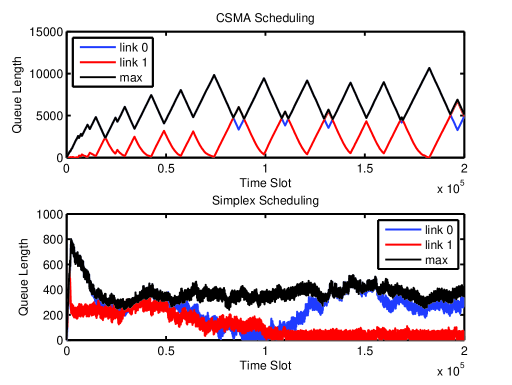
Figure 2: The simulation result of a 7-star network with distributed CSMA scheduling and simplex scheduling.

IV-B Ring Network

We next consider the 6-link ring-shaped interference graph in Fig 1 (b). The simulation result is shown in Fig. 3. Similar to the star network, one can observe that both algorithm result in rate stability, but the simplex scheduling achieves much smaller queue lengths than the distributed CSMA scheduling. In fact, for the ring shaped network, it is easy to see that the optimal modes are $\boldsymbol{\sigma}_{1}=(1,0,1,0,1,0)^{T}$ and $\boldsymbol{\sigma}_{2}=(0,1,0,1,0,1)^{T}$. In the steady state, the simplex scheduler can achieve low delay by quickly switching between these two modes, using the simple max-weight scheduler implemented by average consensus. On the other hand, the switching is much more time-consuming for the distributed CSMA scheduling, due to the random walk based design. Finally, note that the transition time and queue lengths for distributed CSMA scheduling in the 6-ring network is smaller than that for the 7-star network (both have the same arrival rates), due to the fact that, it is easier to switch between the modes in a ring-shaped topology.

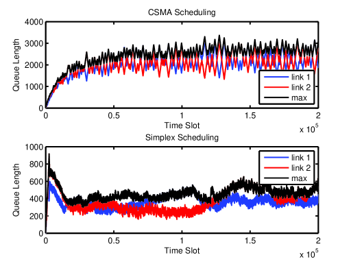
Figure 3: The simulation result of a 6-ring network with different distributed CSMA scheduling and simplex scheduling.

V Conclusion

In this paper, we proposed a distributed throughput-optimal scheduling algorithm for ad hoc wireless networks, which is motivated by the simplex algorithm for solving LP problems. The scheduler maintains a sparse set of basic schedules, and during scheduling, the basic schedule with the maximum weight is selected for transmission in each time slot. The set of basic schedules are updated according to the simplex algorithm, which can be implemented using CSMA mechanisms in a distributed fashion. Compared to the distributed CSMA based scheduling in [1], our algorithm achieves better delay performance in the steady state by allowing faster transitions among the optimal independent sets.

References

- [1] L. Jiang and J. Walrand, “A Distributed CSMA Algorithm for Throughput and Utility Maximization in Wireless Networks,” IEEE/ACM Trans. Networking. Vol. 18, No.3, pp. 960 - 972, Jun. 2010.
- [2] L. Tassiulas and A. Ephremides, “Stability properties of constrained queueing systems and scheduling policies for maximum throughput in multihop radio networks,” IEEE Trans. Automatic Control, Vol. 37, No. 12, pp. 1936-1949, Dec. 1992
- [3] L. Tassiulas, “Linear Complexity Algorithms for Maximum Througput in Radio Networks and Input Queued Switches,” Proc. IEEE INFOCOM, 533-539, 1998
- [4] D. Shah, D. N. C. Tse and J. N. Tsitsiklis, “Hardness of Low Delay Network Scheduling,” Under Submission.
- [5] P. Chaporkar, K. Kar, X. Luo, and S. Sarkar, “Throughput and Fairness Guarantees Through Maximal Scheduling in Wireless Networks”, IEEE Trans. Info. Theory, Vol. 54, No. 2, pp. 572-594, Feb. 2008.
- [6] Q. Li and R. Negi, “Prioritized Maximal Scheduling in Wireless Networks”, Proc. IEEE Globecom, 2008
- [7] Q. Li and R. Negi, “Greedy Maximal Scheduling in Wireless Networks”, Proc. IEEE Globecom, Dec. 2010.
- [8] J. Ni, B. Tan and R. Srikant, “Q-CSMA: Queue length-based CSMA/CA algorithms for achieving maximum throughput and low delay in wireless networks”, Tech Report, available at http://arxiv.org/abs/0901.2333.
- [9] J. Shin and D. Shah, “Randomized Scheduling Algorithm for Queueing Networks,” Under Submission, 2009.
- [10] Libin Jiang, Devavrat Shah, Jinwoo Shin, and Jean Walrand, “Distributed Random Access Algorithm: Scheduling and Congestion Control,” IEEE Trans. on Info. Theory.
- [11] D. Bertsimas and J. N. Tsitsiklis, “Introduction to Linear Optimization”, Dynamic Ideas and Athena Scientific, March 2008.
- [12] D. P. Bertsekas, A. Nedic and A. E. Ozdaglar “Convex Analysis and Optimization”, Athena Scientific, 2003.