Generating Probability Distributions using Multivalued Stochastic Relay Circuits

David Lee Dept. of Electrical Engineering
Stanford University
Palo Alto, CA 94305
Email: davidtlee@stanford.edu
   Jehoshua Bruck Dept. of Electrical Engineering
California Institute of Technology
Pasadena, CA 91125
Email: bruck@caltech.edu
Abstract

The problem of random number generation dates back to von Neumann’s work in 1951. Since then, many algorithms have been developed for generating unbiased bits from complex correlated sources as well as for generating arbitrary distributions from unbiased bits. An equally interesting, but less studied aspect is the structural component of random number generation as opposed to the algorithmic aspect. That is, given a network structure imposed by nature or physical devices, how can we build networks that generate arbitrary probability distributions in an optimal way?

In this paper, we study the generation of arbitrary probability distributions in multivalued relay circuits, a generalization in which relays can take on any of N𝑁N states and the logical ‘and’ and ‘or’ are replaced with ‘min’ and ‘max’ respectively. Previous work was done on two-state relays. We generalize these results, describing a duality property and networks that generate arbitrary rational probability distributions. We prove that these networks are robust to errors and design a universal probability generator which takes input bits and outputs arbitrary binary probability distributions.

I Introduction

I-A Motivation

Many biological systems involve stochasticity. Examples of these include gene expression[4], chemical reactions[5], and neuron signaling[6]. However, despite the stochasticity, often deemed as noise, they are still capable of achieving functionalities that artificial systems cannot yet compete with.

Motivated by the idea that stochasticity is an important enabler of biological computation, we tackle a simpler question as a stepping stone: Can we design networks that generate stochasticity in a systematic way?

I-B Structural Aspects of Random Number Generation

This question is strongly connected to an important thread of work in computer science on random number generation. In 1951, Von Neumann [1] studied this problem in the context of generating a fair coin toss from a biased coin. Knuth and Yao [2] studied the reverse problem of generating arbitrary distributions from unbiased bits (fair coins), which was extended by Han and Hoshi [3] to generating arbitrary distributions from biased distributions. These primarily focus on an algorithmic perspective to random number generation.

In a biological system (or other physical device), we do not have the full generality of the algorithmic approach to generating probability distributions. Randomness arises in specific areas that can only propagate according to the structure of how components are composed in the given network. The study of random number generation under these constraints can be greatly beneficial to understanding natural stochastic systems as well as to designing devices for random number generation. In this paper, we will analyze random number generation in the context of multivalued relay circuits, a generalization of standard relay circuits to any number of states. This generalization is very natural and has an intuitive understanding as the timing of events that have dependencies on other events.

I-C Deterministic Relays
Refer to caption
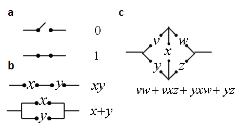
Figure 1: Deterministic Examples. For two states, xy𝑥𝑦xy is the boolean ‘and’ of x𝑥x and y𝑦y while x+y𝑥𝑦x+y is the boolean ‘or’. Figures b and c also apply to multivalued relays where xy𝑥𝑦xy is min(x,y)𝑚𝑖𝑛𝑥𝑦min(x,y) and x+y𝑥𝑦x+y is max(x,y)𝑚𝑎𝑥𝑥𝑦max(x,y). (a) A relay can either be opened (state 0) or closed (state 1). (b) In series, the entire circuit can only be closed if both x𝑥x and y𝑦y are closed. In parallel, the entire circuit will be closed if either x𝑥x or y𝑦y are closed. (c) In this example of a non-sp circuit, we take the boolean ‘and’ along the four possible paths, and then apply the boolean ‘or’ to those subsequent values.

We will start by introducing deterministic relays. A deterministic relay switch is a 2 terminal object which can be connected (closed) by a wire or left open. The state of the switch, which can be either 0 or 1, describes an open or closed state respectively (see Figure 1a). These states are complements of each other. That is, if switch x𝑥x is in state 0, then the complement x¯¯𝑥\bar{x} is in state 1 and vice versa. When multiple switches are composed together, these networks are known as relay circuits. One of these, a series composition, is formed when two switches are put end to end. A parallel composition is formed when two switches are composed so that the beginning terminals are connected together and the end terminals are connected together.

Shannon showed that the series and parallel compositions can be represented by the boolean ‘and’ and ‘or’ operations[8]. If switches x𝑥x and y𝑦y are composed in series to form z1subscript𝑧1z_{1}, then z1subscript𝑧1z_{1} will only be closed if both x𝑥x and y𝑦y are closed. On the other hand, if switches x𝑥x and y𝑦y are composed in parallel to form z2subscript𝑧2z_{2}, then z2subscript𝑧2z_{2} will be closed if either x𝑥x or y𝑦y are closed. We will denote the series composition of x𝑥x and y𝑦y by xy𝑥𝑦x*y or simply xy𝑥𝑦xy and the parallel composition by x+y𝑥𝑦x+y (see Figure 1b). This notation will be preserved for further generalizations of the relay circuits.

Circuits formed solely by series and parallel compositions are called sp circuits. Shannon showed that non sp circuits could also be represented by boolean operations. The general mathematical representation of any relay circuits would be to find all paths that go from the beginning to the end terminal. For each path, we take the boolean ‘and’ of all switches along that path; then we take the boolean ‘or’ of the values derived for each path (see Figure 1c).

I-D Stochastic Relays
Refer to caption
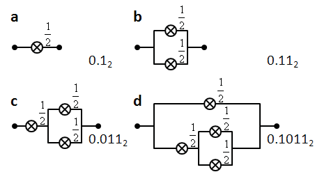
Figure 2: Simple Examples. As stated, 1212\frac{1}{2} is short for (12,12)1212(\frac{1}{2},\frac{1}{2}). (a) A single 1212\frac{1}{2}-pswitch. (b) Putting (a) in parallel with a 1212\frac{1}{2}-pswitch gives 3434\frac{3}{4}. (c) Putting (b) in series with a 1212\frac{1}{2}-pswitch gives 3838\frac{3}{8}. (d) Putting (c) in parallel with a 1212\frac{1}{2}-pswitch gives 11161116\frac{11}{16}.

Recently, Wilhelm and Bruck introduced the notion of a stochastic relay circuit[9]. These circuits are a generalization of Shannon’s relay circuits; instead of having deterministic relay switches that are in either the open or closed state, stochastic relay circuits can exist in either state with a specified probability. If a stochastic relay switch x𝑥x, called a pswitch, has probability p𝑝p of being closed and probability 1p1𝑝1-p of being open, this distribution is represented by a vector v=(1p,p)𝑣1𝑝𝑝v=(1-p,p) where visubscript𝑣𝑖v_{i} corresponds to the probability of x𝑥x being in state i𝑖i. We say that x𝑥x realizes (1p,p)1𝑝𝑝(1-p,p) or simply x𝑥x realizes p𝑝p. If pswitches x𝑥x and y𝑦y, which realize probabilities p𝑝p and q𝑞q respectively, are composed in series, the new composition will realize pq𝑝𝑞pq. If they are composed in parallel, the new composition will realize p+qpq𝑝𝑞𝑝𝑞p+q-pq (see Figure 2).

One of the primary questions dealt with in their work was the generation of probability distributions using a limited number of base switch types, known as a switch set. For example, if the switch set S ={12}absent12=\{\frac{1}{2}\}, then relay circuits built with this switch set can only use pswitches with the distribution (12,12)1212(\frac{1}{2},\frac{1}{2}). They proved that using the switch set S ={12}absent12=\{\frac{1}{2}\}, all probability distributions a2n𝑎superscript2𝑛\frac{a}{2^{n}} could be realized with at most n𝑛n pswitches. Continuing, many more results were proved not only in realizing other probability distributions[9][10], but also in circuit constructions such as a Universal Probability Generator[9] and in robustness[11] and expressibility[10] properties of these circuits.

I-E Multivalued Stochastic Relays

In order to study non-bernoulli random variables, it is necessary to generalize Shannon’s relays to a larger number of states. Multivalued logics have been studied as early as in 1921 by Post[12] and followed up on by Webb[13] and others[14]. The work presented in this paper concerns one generalization of two-state relay circuits to multivalued relay circuits where we use two multivalued functions (gates).

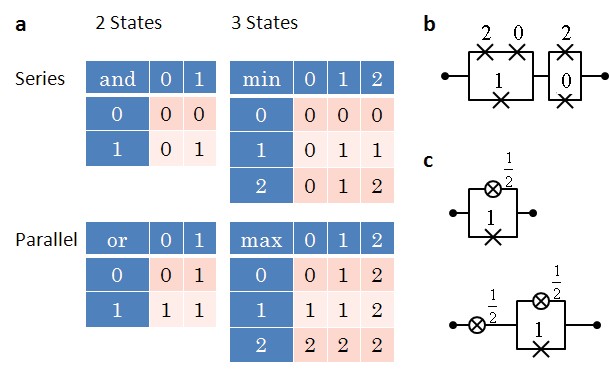
A multivalued switch is a relay switch that can be in any of n states: 0, 1, 2, …, n-1. We define the complement of a switch to be n1i𝑛1𝑖n-1-i, where i𝑖i is the state of the switch. Series and parallel compositions are redefined to ‘min’ and ‘max’, respectively, rather than the boolean ‘and’ and ‘or’. This means that when switches x𝑥x and y𝑦y are composed in series, the overall circuit is in state min(x,y)𝑥𝑦\min(x,y) and when they are composed in parallel, the overall circuit is in state max(x,y)𝑥𝑦\max(x,y) (see Figure 3a and b). Non-sp circuits are also defined in a similar way to 2-state circuits. The general mathematical representation of any multivalued relay circuit is to find all paths that go from the beginning to the end terminal. For each path, we take the ‘min’ of all switches along that path; then we take the ‘max’ of the values derived for each path (Figures 1b and c still apply).
Refer to caption
Figure 3: 3-state Examples. We use ×\times to represent a deterministic switch and tensor-product\otimes to represent a pswitch. (a) A comparison of the truth tables for 2-state and 3-state relay switches. (b) A simple 3-state deterministic example. Evaluating series connections using min and parallel connections as max, we find that this circuit is in state 1. (c) A simple 3-state stochastic example. On the top, we put a (12,0,12)12012(\frac{1}{2},0,\frac{1}{2}) pswitch in parallel with a deterministic switch in state 1. Then, with 1212\frac{1}{2} probability we get max(0,1)01\max(0,1) and with 1212\frac{1}{2} probability we get max(2,1)21\max(2,1), which yields a (0,12,12)01212(0,\frac{1}{2},\frac{1}{2}) circuit. Similarly, we can calculate the bottom circuit to realize distribution (12,14,14)121414(\frac{1}{2},\frac{1}{4},\frac{1}{4}).

One physical understanding of this max-min algebra is found in the timing of relay switches. Let a switch start off in the closed position. Then the state of the switch will be the time t{0,1,,n1}𝑡01𝑛1t\in\{0,1,...,n-1\} when the switch opens. Compose two switches, which open at time t1subscript𝑡1t_{1} and t2subscript𝑡2t_{2}, in series. If either switch opens, then the overall connection is broken. Therefore, the time that the series composition will be open is min(t1,t2)subscript𝑡1subscript𝑡2\min(t_{1},t_{2}). In the same way, we can compose the switches in parallel. Since both switches need to be opened in order for the overall circuit to be open, the time calculated for the parallel composition is max(t1,t2)subscript𝑡1subscript𝑡2\max(t_{1},t_{2}). More generally, the max-min algebra can be used to understand the timing of events when an event occurence depends on the occurence of other events, i.e. event A𝐴A occurs if event B𝐵B occurs or if event C𝐶C and D𝐷D occur. Max-min functions have been studied as a way of reasoning about discrete event systems[15].

Now that we have defined multivalued relays, we can also reason about probability distributions over the n𝑛n states of a multivalued stochastic relay. If a 3-state pswitch x𝑥x has probability p0subscript𝑝0p_{0} of being in state 0, p1subscript𝑝1p_{1} of being in state 1, and p2subscript𝑝2p_{2} of being in state 2, we represent the distribution with the vector v=(p0,p1,p2)𝑣subscript𝑝0subscript𝑝1subscript𝑝2v=(p_{0},p_{1},p_{2}) and say x𝑥x realizes (p0,p1,p2)subscript𝑝0subscript𝑝1subscript𝑝2(p_{0},p_{1},p_{2}). If the distribution is in the form (1p,0,,0,p)1𝑝00𝑝(1-p,0,...,0,p), we will shorten this to simply p𝑝p if the number of states can be inferred from the context or if the equation holds for any number of states (see Figure 3c).

We present the following results in our paper:

  1. 1.

    A duality property (Section II).

  2. 2.

    Networks for generating binary probability distributions (Sections III and IV).

  3. 3.

    Networks for generating rational distributions (Section V).

  4. 4.

    Robustness of the previous networks to switch errors (Section VI).

  5. 5.

    Universal Probability Generation (Section VII).

  6. 6.

    Switching with partially ordered states (Section VIII).

  7. 7.

    Applications to neural circuits and DNA Computing (Section IX).

II Duality

It is important to characterize properties of multivalued circuits. One well-known property is duality, which plays a role in resistor networks, deterministic and two-state stochastic relay circuits. We show that a similar duality concept exists for multivalued circuits. Define the dual state of i𝑖i as the state n1i𝑛1𝑖n-1-i; the dual distribution of v𝑣v as the distribution v¯¯𝑣\bar{v} where v¯i=vn1isubscript¯𝑣𝑖subscript𝑣𝑛1𝑖\bar{v}_{i}=v_{n-1-i}; the dual switch of x𝑥x as the switch x¯¯𝑥\bar{x} that realizes the dual distribution of x𝑥x; and the dual circuit of C𝐶C as the circuit C¯¯𝐶\bar{C} that realizes the dual distribution of C𝐶C.

Refer to caption
Figure 4: 3-state Duality Example. Remember that the 3-state 1212\frac{1}{2}-pswitch is the shorthand for the (12,0,12)12012(\frac{1}{2},0,\frac{1}{2}) pswitch. (a) A two element duality example. (b) A duality example on a larger circuit. Note that since the pswitches are symmetric distributions (duals of themselves), only the compositions are changed.
Theorem 1 (Duality Theorem)

Given a stochastic series-parallel circuit C𝐶C, we can construct C¯¯𝐶\bar{C} by replacing all the switches in C𝐶C with their dual switches and by replacing series connections with parallel connections and vice versa. (see Figure 4).

Proof:

This is shown using induction on series-parallel connections.

Base Case: The dual of a single pswitch with distribution (p0,p1,,pn1)subscript𝑝0subscript𝑝1subscript𝑝𝑛1(p_{0},p_{1},...,p_{n-1}) is (pn1,,p1,p0)subscript𝑝𝑛1subscript𝑝1subscript𝑝0(p_{n-1},...,p_{1},p_{0}), which trivially satisfies the theorem.

Inductive Step: Suppose a circuit C𝐶C with distribution (p0,p1,,pn1)subscript𝑝0subscript𝑝1subscript𝑝𝑛1(p_{0},p_{1},...,p_{n-1}) and a circuit Csuperscript𝐶C^{\prime} with distribution (q0,q1,,qn1)subscript𝑞0subscript𝑞1subscript𝑞𝑛1(q_{0},q_{1},...,q_{n-1}) satisfy the theorem, i.e. the distribution of C¯¯𝐶\bar{C} is (pn1,,p1,p0)subscript𝑝𝑛1subscript𝑝1subscript𝑝0(p_{n-1},...,p_{1},p_{0}) and the distribution of C¯¯superscript𝐶\bar{C^{\prime}} is (qn1,,q1,q0)subscript𝑞𝑛1subscript𝑞1subscript𝑞0(q_{n-1},...,q_{1},q_{0}). To prove the theorem, it is sufficient for us to show that CC𝐶superscript𝐶CC^{\prime} is the dual of C¯+C¯¯𝐶¯superscript𝐶\bar{C}+\bar{C^{\prime}}.

Let Cs=CCsubscript𝐶𝑠𝐶superscript𝐶C_{s}=CC^{\prime} and Cp=C¯+C¯subscript𝐶𝑝¯𝐶¯superscript𝐶C_{p}=\bar{C}+\bar{C^{\prime}}. Then Cs=(c0,c1,,cn1)subscript𝐶𝑠subscript𝑐0subscript𝑐1subscript𝑐𝑛1C_{s}=(c_{0},c_{1},...,c_{n-1}) and Cp=(d0,d1,,dn1)subscript𝐶𝑝subscript𝑑0subscript𝑑1subscript𝑑𝑛1C_{p}=(d_{0},d_{1},...,d_{n-1}) where

cksubscript𝑐𝑘\displaystyle\displaystyle c_{k} =min(i,j)=kPr(C=i)Pr(C=j)absentsubscript𝑚𝑖𝑛𝑖𝑗𝑘𝑃𝑟𝐶𝑖𝑃𝑟superscript𝐶𝑗\displaystyle=\sum\limits_{min(i,j)=k}Pr(C=i)Pr(C^{\prime}=j)
=min(i,j)=kpiqjabsentsubscript𝑚𝑖𝑛𝑖𝑗𝑘subscript𝑝𝑖subscript𝑞𝑗\displaystyle=\sum\limits_{min(i,j)=k}p_{i}q_{j}
dksubscript𝑑𝑘\displaystyle d_{k} =max(i,j)=kPr(C¯=i)Pr(C¯=j)absentsubscript𝑚𝑎𝑥𝑖𝑗𝑘𝑃𝑟¯𝐶𝑖𝑃𝑟¯superscript𝐶𝑗\displaystyle=\sum\limits_{max(i,j)=k}Pr(\bar{C}=i)Pr(\bar{C^{\prime}}=j)
=max(i,j)=kpn1iqn1jabsentsubscript𝑚𝑎𝑥𝑖𝑗𝑘subscript𝑝𝑛1𝑖subscript𝑞𝑛1𝑗\displaystyle=\sum\limits_{max(i,j)=k}p_{n-1-i}q_{n-1-j}
=min(n1i,n1j)=n1kpn1iqn1jabsentsubscript𝑚𝑖𝑛𝑛1𝑖𝑛1𝑗𝑛1𝑘subscript𝑝𝑛1𝑖subscript𝑞𝑛1𝑗\displaystyle=\sum\limits_{min(n-1-i,n-1-j)=n-1-k}p_{n-1-i}q_{n-1-j}
=min(i,j)=n1kpiqjabsentsubscript𝑚𝑖𝑛superscript𝑖superscript𝑗𝑛1𝑘subscript𝑝superscript𝑖subscript𝑞superscript𝑗\displaystyle=\sum\limits_{min(i^{\prime},j^{\prime})=n-1-k}p_{i^{\prime}}q_{j^{\prime}}
=cn1k.absentsubscript𝑐𝑛1𝑘\displaystyle=c_{n-1-k}.

We see that d0=cn1subscript𝑑0subscript𝑐𝑛1d_{0}=c_{n-1}, d1=cn2subscript𝑑1subscript𝑐𝑛2d_{1}=c_{n-2}, …, dn1=c0subscript𝑑𝑛1subscript𝑐0d_{n-1}=c_{0}, demonstrating that Cssubscript𝐶𝑠C_{s} is the dual of Cpsubscript𝐶𝑝C_{p}. ∎

III Realizing Binary 3-state Distributions

We can now ask questions about generating probability distributions with stochastic relay circuits. These include: What are the possible distributions that can be realized? What is the smallest set of basic switching elements necessary to realize these distributions? Are there efficient constructions to realize these distributions? We will begin by demonstrating how to generate distributions on 3 states.

In writing out algorithms and circuit constructions we will use the notation introduced earlier for series and parallel connections, i.e. xy𝑥𝑦xy and x+y𝑥𝑦x+y will denote series and parallel connections respectively. We will use this notation loosely, i.e., (12,0,12)(12,12,0)1201212120(\frac{1}{2},0,\frac{1}{2})(\frac{1}{2},\frac{1}{2},0) represents a circuit formed by composing a (12,0,12)12012(\frac{1}{2},0,\frac{1}{2}) pswitch in series with a (12,12,0)12120(\frac{1}{2},\frac{1}{2},0) pswitch.

Lemma 1 (3-state sp composition rules)

Given p=(p0,p1,p2)𝑝subscript𝑝0subscript𝑝1subscript𝑝2p=(p_{0},p_{1},p_{2}) and q=(q0,q1,q2)𝑞subscript𝑞0subscript𝑞1subscript𝑞2q=(q_{0},q_{1},q_{2}), let x=pq𝑥𝑝𝑞x=pq and y=p+q𝑦𝑝𝑞y=p+q. Then,

x0subscript𝑥0\displaystyle\displaystyle x_{0} =p0q0+p0q1+p0q2+p1q0+p2q0absentsubscript𝑝0subscript𝑞0subscript𝑝0subscript𝑞1subscript𝑝0subscript𝑞2subscript𝑝1subscript𝑞0subscript𝑝2subscript𝑞0\displaystyle=p_{0}q_{0}+p_{0}q_{1}+p_{0}q_{2}+p_{1}q_{0}+p_{2}q_{0}
=1(1p0)(1q0)absent11subscript𝑝01subscript𝑞0\displaystyle=1-(1-p_{0})(1-q_{0})
x1subscript𝑥1\displaystyle x_{1} =p1q1+p1q2+p2q1absentsubscript𝑝1subscript𝑞1subscript𝑝1subscript𝑞2subscript𝑝2subscript𝑞1\displaystyle=p_{1}q_{1}+p_{1}q_{2}+p_{2}q_{1}
x2subscript𝑥2\displaystyle x_{2} =p2q2absentsubscript𝑝2subscript𝑞2\displaystyle=p_{2}q_{2}
y0subscript𝑦0\displaystyle y_{0} =p0q0absentsubscript𝑝0subscript𝑞0\displaystyle=p_{0}q_{0}
y1subscript𝑦1\displaystyle y_{1} =p1q1+p1q0+p0q1absentsubscript𝑝1subscript𝑞1subscript𝑝1subscript𝑞0subscript𝑝0subscript𝑞1\displaystyle=p_{1}q_{1}+p_{1}q_{0}+p_{0}q_{1}
y2subscript𝑦2\displaystyle y_{2} =p2q2+p2q1+p2q0+p1q2+p0q2absentsubscript𝑝2subscript𝑞2subscript𝑝2subscript𝑞1subscript𝑝2subscript𝑞0subscript𝑝1subscript𝑞2subscript𝑝0subscript𝑞2\displaystyle=p_{2}q_{2}+p_{2}q_{1}+p_{2}q_{0}+p_{1}q_{2}+p_{0}q_{2}
=1(1p2)(1q2)absent11subscript𝑝21subscript𝑞2\displaystyle=1-(1-p_{2})(1-q_{2})
Proof:

The above expressions follow from enumerating all 32superscript323^{2} switch combinations. ∎

Refer to caption
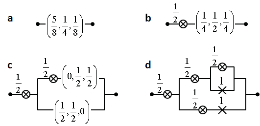
Figure 5: Realizing 3-state Distribution. (a) We want to realize (58,14,18)581418(\frac{5}{8},\frac{1}{4},\frac{1}{8}). This falls under the first case. (b) Now we have an unconstructed distribution that falls under the second case. (c) There are two unconstructed distributions. The top one falls under case 3 and the bottom falls under case 2. (Note that case 2 is equivalent to case 1 for p0=12subscript𝑝012p_{0}=\frac{1}{2}). (d) The final circuit.
Theorem 2 (Binary 3-state Distributions)

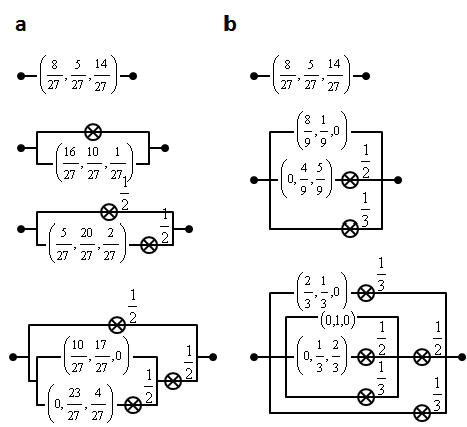
Using the switch set S ={12}absent12=\{\frac{1}{2}\} and the deterministic switches, we can realize all 3-state distributions of the form (a2n,b2n,c2n)𝑎superscript2𝑛𝑏superscript2𝑛𝑐superscript2𝑛(\frac{a}{2^{n}},\frac{b}{2^{n}},\frac{c}{2^{n}}) using at most 2n12𝑛12n-1 pswitches with the following recursive circuit construction (see Figure 5 for an example):

  if pS𝑝𝑆p\in S then
     return p𝑝p
  else if a2n>12𝑎superscript2𝑛12\frac{a}{2^{n}}>\frac{1}{2} then
     return (12,0,12)(a2n12n1,b2n1,c2n1)12012𝑎superscript2𝑛1superscript2𝑛1𝑏superscript2𝑛1𝑐superscript2𝑛1(\frac{1}{2},0,\frac{1}{2})(\frac{a-2^{n-1}}{2^{n-1}},\frac{b}{2^{n-1}},\frac{c}{2^{n-1}})
  else if a+b2n>12𝑎𝑏superscript2𝑛12\frac{a+b}{2^{n}}>\frac{1}{2} then
     return (a2n1,2n1a2n1,0)+(12,0,12)(0,2n1c2n1,c2n1)𝑎superscript2𝑛1superscript2𝑛1𝑎superscript2𝑛10120120superscript2𝑛1𝑐superscript2𝑛1𝑐superscript2𝑛1(\frac{a}{2^{n-1}},\frac{2^{n-1}-a}{2^{n-1}},0)+(\frac{1}{2},0,\frac{1}{2})(0,\frac{2^{n-1}-c}{2^{n-1}},\frac{c}{2^{n-1}})
  else if a+b+c2n>12𝑎𝑏𝑐superscript2𝑛12\frac{a+b+c}{2^{n}}>\frac{1}{2} then
     return (a2n1,b2n1,c2n12n1)+(12,0,12)𝑎superscript2𝑛1𝑏superscript2𝑛1𝑐superscript2𝑛1superscript2𝑛112012(\frac{a}{2^{n-1}},\frac{b}{2^{n-1}},\frac{c-2^{n-1}}{2^{n-1}})+(\frac{1}{2},0,\frac{1}{2})
  end if
Proof:

For any distribution p=(p0,p1,p2)𝑝subscript𝑝0subscript𝑝1subscript𝑝2p=(p_{0},p_{1},p_{2}), there exists some smallest k𝑘k such that i=0kpi>12superscriptsubscript𝑖0𝑘subscript𝑝𝑖12\sum_{i=0}^{k}p_{i}>\frac{1}{2}, which correspond to the 3 recursive cases enumerated above. We can verify that for each of these cases:

  1. 1.

    The decompositions obey the 3-state composition rules.

  2. 2.

    The switches are valid (non-negative probabilities and sum to 1)

Since each algorithm’s decomposition uses switches of type (a2n1,b2n1,c2n1)𝑎superscript2𝑛1𝑏superscript2𝑛1𝑐superscript2𝑛1(\frac{a}{2^{n-1}},\frac{b}{2^{n-1}},\frac{c}{2^{n-1}}), then we will eventually have n=0𝑛0n=0, corresponding to a deterministic switch; at this point the algorithm terminates and has successfully constructed any (a2n,b2n,c2n)𝑎superscript2𝑛𝑏superscript2𝑛𝑐superscript2𝑛(\frac{a}{2^{n}},\frac{b}{2^{n}},\frac{c}{2^{n}}).

Refer to caption
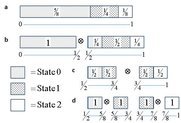
Figure 6: Block-Interval visualization of 3-state Algorithm. We want to realize (58,14,18)581418(\frac{5}{8},\frac{1}{4},\frac{1}{8}). A tensor-product\otimes symbol marks where the cuts occur which correspond to the use of one pswitch. (a) We start with one interval split into blocks corresponding to the pswitch probabilities. (b) When we cut [0,1]01[0,1] in half, we get two intervals; the blocks are cut and the probabilities change according to the new interval size. (c) The second application of the algorithm. (d) When we are left with single block-interval pairs, we know we are done since the deterministic switch is in our switch set.

We will now prove that we use at most 2n12𝑛12n-1 pswitches for all n1𝑛1n\geq 1. Define fnsubscript𝑓𝑛f_{n} as the maximum number of pswitches used in the construction of any distribution (a2n,b2n,c2n)𝑎superscript2𝑛𝑏superscript2𝑛𝑐superscript2𝑛(\frac{a}{2^{n}},\frac{b}{2^{n}},\frac{c}{2^{n}}). Then,

f1subscript𝑓1\displaystyle\displaystyle f_{1} =1absent1\displaystyle=1 (1)
fnsubscript𝑓𝑛\displaystyle f_{n} =max(fn1+1,2(n1)+1,fn1+1)absentsubscript𝑓𝑛112𝑛11subscript𝑓𝑛11\displaystyle=\max(f_{n-1}+1,2(n-1)+1,f_{n-1}+1) (2)
=max(fn1+1,2n1)absentsubscript𝑓𝑛112𝑛1\displaystyle=\max(f_{n-1}+1,2n-1)

where (1) is shown trivially, and (2) is derived from the 3 cases of the algorithm. Note that we are using a previous result[9] that 2 state distributions of form (a2n,b2n)𝑎superscript2𝑛𝑏superscript2𝑛(\frac{a}{2^{n}},\frac{b}{2^{n}}) use at most n𝑛n switches, and also assuming here that our algorithm generalizes the previous algorithm; that is, distributions of the form (a2n,b2n,0)𝑎superscript2𝑛𝑏superscript2𝑛0(\frac{a}{2^{n}},\frac{b}{2^{n}},0) and its permutations also use at most n𝑛n switches – this application of their 2-state proof to our multivalued distribution is sound as will be explained more rigorously in the following section. We are now left with a simple induction exercise.

Base Case: f1=1=2(1)1subscript𝑓11211f_{1}=1=2(1)-1.

Inductive Step: Assume fk=2k1subscript𝑓𝑘2𝑘1f_{k}=2k-1. Then,

fk+1subscript𝑓𝑘1\displaystyle f_{k+1} =max(fk+1,2(k+1)1)absentsubscript𝑓𝑘12𝑘11\displaystyle=\max(f_{k}+1,2(k+1)-1)
=max(2k,2(k+1)1)absent2𝑘2𝑘11\displaystyle=\max(2k,2(k+1)-1)
=2(k+1)1.absent2𝑘11\displaystyle=2(k+1)-1.

So fk=2k1fk+1=2(k+1)1subscript𝑓𝑘2𝑘1subscript𝑓𝑘12𝑘11f_{k}=2k-1\implies f_{k+1}=2(k+1)-1. ∎

It is useful at this time to provide some intuition regarding the algorithm. We can view the original distribution as a series of blocks dividing up the interval [0,1]01[0,1] (see Figure 6). By applying the algorithm, we are separating this larger interval into smaller intervals [0,12]012[0,\frac{1}{2}] and [12,1]121[\frac{1}{2},1], cutting any blocks on that boundary. When this separation occurs, the total size of the block is decreased (namely, in half), and so the probabilities representing those intervals change - these probabilities are precisely those of the algorithm. Namely, we can rewrite the three cases of the algorithm:

(a2n,b2n,c2n)=𝑎superscript2𝑛𝑏superscript2𝑛𝑐superscript2𝑛absent\displaystyle\textstyle{(\frac{a}{2^{n}},\frac{b}{2^{n}},\frac{c}{2^{n}})}=
Case 1: (1,0,0)+(12,0,12)(a2n12n1,b2n1,c2n1)10012012𝑎superscript2𝑛1superscript2𝑛1𝑏superscript2𝑛1𝑐superscript2𝑛1\displaystyle\textstyle{(1,0,0)+(\frac{1}{2},0,\frac{1}{2})(\frac{a-2^{n-1}}{2^{n-1}},\frac{b}{2^{n-1}},\frac{c}{2^{n-1}})}
Case 2: (a2n1,2n1a2n1,0)+(12,0,12)(0,2n1c2n1,c2n1)𝑎superscript2𝑛1superscript2𝑛1𝑎superscript2𝑛10120120superscript2𝑛1𝑐superscript2𝑛1𝑐superscript2𝑛1\displaystyle\textstyle{(\frac{a}{2^{n-1}},\frac{2^{n-1}-a}{2^{n-1}},0)+(\frac{1}{2},0,\frac{1}{2})(0,\frac{2^{n-1}-c}{2^{n-1}},\frac{c}{2^{n-1}})}
Case 3: (a2n1,b2n1,c2n12n1)+(12,0,12)(0,0,1)𝑎superscript2𝑛1𝑏superscript2𝑛1𝑐superscript2𝑛1superscript2𝑛112012001\displaystyle\textstyle{(\frac{a}{2^{n-1}},\frac{b}{2^{n-1}},\frac{c-2^{n-1}}{2^{n-1}})+(\frac{1}{2},0,\frac{1}{2})(0,0,1)}

IV Realizing Binary N𝑁N-state Distributions

We are now ready to continue with our algorithm for N𝑁N states. Intuitively, we can describe the algorithm for N𝑁N states in the same way as for 3 states. We first find the smallest index k𝑘k for which i=0kpi>12superscriptsubscript𝑖0𝑘subscript𝑝𝑖12\sum_{i=0}^{k}p_{i}>\frac{1}{2}. Then based on the index k𝑘k, we can decompose our distribution in a way corresponding to the interval-block visualization; the only difference is that each interval can now have up to N𝑁N block-types instead of just 3.

Refer to caption
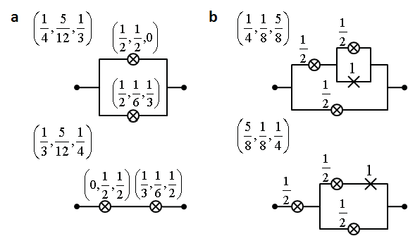
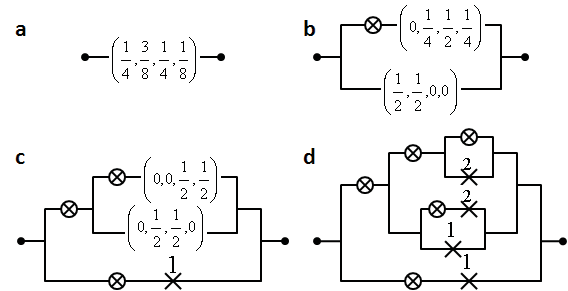
Figure 7: Realizing 4-state Distribution. We use the N𝑁N-state algorithm on the a 4-state distribution. A tensor-product\otimes symbol represents the pswitch (12,0,0,12)120012(\frac{1}{2},0,0,\frac{1}{2}). (a) We want to realize (14,38,14,18)14381418(\frac{1}{4},\frac{3}{8},\frac{1}{4},\frac{1}{8}). Initially, p0+p1>12subscript𝑝0subscript𝑝112p_{0}+p_{1}>\frac{1}{2}. (b) For the top distribution, p0+p1+p2>12subscript𝑝0subscript𝑝1subscript𝑝212p_{0}+p_{1}+p_{2}>\frac{1}{2}. For the bottom distribution, p0+p1>12subscript𝑝0subscript𝑝112p_{0}+p_{1}>\frac{1}{2}. (c) For the top distribution, p0+p1+p2+p3>12subscript𝑝0subscript𝑝1subscript𝑝2subscript𝑝312p_{0}+p_{1}+p_{2}+p_{3}>\frac{1}{2}. For the bottom distribution, p0+p1+p2>12subscript𝑝0subscript𝑝1subscript𝑝212p_{0}+p_{1}+p_{2}>\frac{1}{2}. (d) The final circuit.
Theorem 3 (Binary N-state Distributions)

Using the switch set S ={12}absent12=\{\frac{1}{2}\} and the deterministic switches, we can realize all N𝑁N-state distributions of the form (x02n,x12n,,xN12n)subscript𝑥0superscript2𝑛subscript𝑥1superscript2𝑛subscript𝑥𝑁1superscript2𝑛(\frac{x_{0}}{2^{n}},\frac{x_{1}}{2^{n}},...,\frac{x_{N-1}}{2^{n}}) with at most fn,N=subscript𝑓𝑛𝑁absentf_{n,N}=

{2n1,nlog2N2log2N1+(N1)(nlog2N),nlog2Ncasessuperscript2𝑛1𝑛subscript2𝑁superscript2subscript2𝑁1𝑁1𝑛subscript2𝑁𝑛subscript2𝑁\displaystyle\begin{cases}2^{n}-1,&n\leq\lceil\log_{2}N\rceil\\ 2^{\lceil\log_{2}N\rceil}-1+(N-1)(n-\lceil\log_{2}N\rceil),&n\geq\lceil\log_{2}N\rceil\end{cases}

switches, using the following recursive circuit construction (see Figure 7):

Algorithm 1 Note that we are using 1212\frac{1}{2} as a shorthand for (12,,12)1212(\frac{1}{2},...,\frac{1}{2}) as explained in the introduction.
  if pS𝑝𝑆p\in S then
     return p𝑝p
  else if x02n>12subscript𝑥0superscript2𝑛12\frac{x_{0}}{2^{n}}>\frac{1}{2} then
     return 12(x02n12n1,x12n1,,xN12n1)12subscript𝑥0superscript2𝑛1superscript2𝑛1subscript𝑥1superscript2𝑛1subscript𝑥𝑁1superscript2𝑛1\frac{1}{2}(\frac{x_{0}-2^{n-1}}{2^{n-1}},\frac{x_{1}}{2^{n-1}},...,\frac{x_{N-1}}{2^{n-1}})
  else if x0+x12n>12subscript𝑥0subscript𝑥1superscript2𝑛12\frac{x_{0}+x_{1}}{2^{n}}>\frac{1}{2} then
     return (x02n1,2n1x02n1,)+12(0,x0+x12n12n1,x22n1,)subscript𝑥0superscript2𝑛1superscript2𝑛1subscript𝑥0superscript2𝑛1120subscript𝑥0subscript𝑥1superscript2𝑛1superscript2𝑛1subscript𝑥2superscript2𝑛1(\frac{x_{0}}{2^{n-1}},\frac{2^{n-1}-x_{0}}{2^{n-1}},...)+\frac{1}{2}(0,\frac{x_{0}+x_{1}-2^{n-1}}{2^{n-1}},\frac{x_{2}}{2^{n-1}},...)
  else if … then
     …
  else if x0+x1++xN12n>12subscript𝑥0subscript𝑥1subscript𝑥𝑁1superscript2𝑛12\frac{x_{0}+x_{1}+...+x_{N-1}}{2^{n}}>\frac{1}{2} then
     return (x02n1,x12n1,,xN12n12n1)+12subscript𝑥0superscript2𝑛1subscript𝑥1superscript2𝑛1subscript𝑥𝑁1superscript2𝑛1superscript2𝑛112(\frac{x_{0}}{2^{n-1}},\frac{x_{1}}{2^{n-1}},...,\frac{x_{N-1}-2^{n-1}}{2^{n-1}})+\frac{1}{2}
  end if

The algorithm’s correctness can be confirmed from the composition rules for N-states. Before proving the complexity of the above algorithm, we state an intermediate lemma:

Lemma 2

Define an active state of a distribution as a state with non-zero probability. Given any distribution of the form (x02n,x12n,,xN12n)subscript𝑥0superscript2𝑛subscript𝑥1superscript2𝑛subscript𝑥𝑁1superscript2𝑛(\frac{x_{0}}{2^{n}},\frac{x_{1}}{2^{n}},...,\frac{x_{N-1}}{2^{n}}) with mN𝑚𝑁m\leq N active states, the number of pswitches needed to realize the distribution is at most fn,msubscript𝑓𝑛𝑚f_{n,m}.

Proof:

Re-map the m𝑚m active states to 0,1,,m101𝑚10,1,...,m-1 in a way that preserves state order. Since all operations under max\max and min\min are preserved, any distribution on the original m𝑚m active states can be constructed by constructing a distribution on the mapped states and reversing the mapping on the base switches. Therefore, the number of pswitches required cannot be greater than fn,msubscript𝑓𝑛𝑚f_{n,m}. This also gives us insight into fn,Nsubscript𝑓𝑛𝑁f_{n,N} for the region nlog2N𝑛subscript2𝑁n\leq\lceil\log_{2}N\rceil. In this region, the number of active states is limited by n𝑛n, resulting in states with zero probability. Then, it makes sense that the complexity only depends on n𝑛n. ∎

Proof:

We will now prove the complexity of pswitches required. The following recursive relations hold for fn,Nsubscript𝑓𝑛𝑁f_{n,N},

fn,1subscript𝑓𝑛1\displaystyle f_{n,1} =0absent0\displaystyle=0 (3)
f0,Nsubscript𝑓0𝑁\displaystyle f_{0,N} =0absent0\displaystyle=0 (4)
fn,Nsubscript𝑓𝑛𝑁\displaystyle f_{n,N} =max(fn1,1+fn1,N+1,\displaystyle=\max(f_{n-1,1}+f_{n-1,N}+1, (5)
fn1,2+fn1,N1+1,subscript𝑓𝑛12subscript𝑓𝑛1𝑁11\displaystyle f_{n-1,2}+f_{n-1,N-1}+1,
,\displaystyle...,
fn1,N+fn1,1+1)\displaystyle f_{n-1,N}+f_{n-1,1}+1)
=max1iN2(fn1,i+fn1,Ni+1)+1absentsubscript1𝑖𝑁2subscript𝑓𝑛1𝑖subscript𝑓𝑛1𝑁𝑖11\displaystyle=\max_{1\leq i\leq\lceil\frac{N}{2}\rceil}(f_{n-1,i}+f_{n-1,N-i+1})+1 (6)

where (3) and (4) are trivial since both define deterministic switches and (5) comes from an application of the above lemma to the different cases of the algorithm. If we fill out a table based on the recursive relations (see Table I), we find that the values match our closed form hypothesis. To prove it, we will:

  1. 1.

    Demonstrate that (6) is maximized at i=N2𝑖𝑁2i=\lceil\frac{N}{2}\rceil.

  2. 2.

    Use induction to prove fn,Nsubscript𝑓𝑛𝑁f_{n,N} for nlog2N𝑛subscript2𝑁n\leq\lceil\log_{2}N\rceil.

  3. 3.

    Use induction to prove fn,Nsubscript𝑓𝑛𝑁f_{n,N} for nlog2N𝑛subscript2𝑁n\geq\lceil\log_{2}N\rceil.

0 1 2 3 4 5 6 7 8 9 10
1 0 0 0 0 0 0 0 0 0 0 0
2 0 1 2 3 4 5 6 7 8 9 10
3 0 1 3 5 7 9 11 13 15 17 19
4 0 1 3 6 9 12 15 18 21 24 27
5 0 1 3 7 11 15 19 23 27 31 35
6 0 1 3 7 12 17 22 27 32 37 42
7 0 1 3 7 13 19 25 31 37 43 49
8 0 1 3 7 14 21 28 35 42 49 56
9 0 1 3 7 15 23 31 39 47 55 63
TABLE I: (row, column) values correspond to (N𝑁N, n𝑛n). The n=log2N𝑛subscript2𝑁n=\lceil\log_{2}N\rceil border is bolded.

Part 1: Define Δn,N=fn,N+1fn,NsubscriptΔ𝑛𝑁subscript𝑓𝑛𝑁1subscript𝑓𝑛𝑁\Delta_{n,N}=f_{n,N+1}-f_{n,N}.

If nlog2(N+1)𝑛subscript2𝑁1n\geq\lceil\log_{2}(N+1)\rceil,

Δn,NsubscriptΔ𝑛𝑁\displaystyle\Delta_{n,N} =[(nlog2(N+1))(N+11)+2log2(N+1)]absentdelimited-[]𝑛subscript2𝑁1𝑁11superscript2subscript2𝑁1\displaystyle=[(n-\lceil\log_{2}(N+1)\rceil)(N+1-1)+2^{\lceil\log_{2}(N+1)\rceil}]
[(nlog2N)(N1)+2log2N]delimited-[]𝑛subscript2𝑁𝑁1superscript2subscript2𝑁\displaystyle\ \ -[(n-\lceil\log_{2}N\rceil)(N-1)+2^{\lceil\log_{2}N\rceil}]

For N𝑁N a multiple of 2, log2(N+1)=log2N+1subscript2𝑁1subscript2𝑁1\lceil\log_{2}(N+1)\rceil=\lceil\log_{2}N\rceil+1, so

Δn,NsubscriptΔ𝑛𝑁\displaystyle\Delta_{n,N} =[(nlog2N1)N+2log2N+1]absentdelimited-[]𝑛subscript2𝑁1𝑁superscript2subscript2𝑁1\displaystyle=[(n-\lceil\log_{2}N\rceil-1)N+2^{\lceil\log_{2}N\rceil+1}]
[(nlog2N)(N1)+2log2N]delimited-[]𝑛subscript2𝑁𝑁1superscript2subscript2𝑁\displaystyle\ \ -[(n-\lceil\log_{2}N\rceil)(N-1)+2^{\lceil\log_{2}N\rceil}]
=N+nlog2N+Nabsent𝑁𝑛subscript2𝑁𝑁\displaystyle=-N+n-\lceil\log_{2}N\rceil+N
=nlog2Nabsent𝑛subscript2𝑁\displaystyle=n-\lceil\log_{2}N\rceil

For N𝑁N not a multiple of 2, log2(N+1)=log2Nsubscript2𝑁1subscript2𝑁\lceil\log_{2}(N+1)\rceil=\lceil\log_{2}N\rceil, so

Δn,NsubscriptΔ𝑛𝑁\displaystyle\Delta_{n,N} =nlog2Nabsent𝑛subscript2𝑁\displaystyle=n-\lceil\log_{2}N\rceil

If nlog2N𝑛subscript2𝑁n\leq\lceil\log_{2}N\rceil,

Δn,NsubscriptΔ𝑛𝑁\displaystyle\Delta_{n,N} =2n2n=0absentsuperscript2𝑛superscript2𝑛0\displaystyle=2^{n}-2^{n}=0

So we have,

Δn,NsubscriptΔ𝑛𝑁\displaystyle\Delta_{n,N} ={nlog2N,nlog2(N+1)0,nlog2Nabsentcases𝑛subscript2𝑁𝑛subscript2𝑁10𝑛subscript2𝑁\displaystyle=\begin{cases}n-\lceil\log_{2}N\rceil,&n\geq\lceil\log_{2}(N+1)\rceil\\ 0,&n\leq\lceil\log_{2}N\rceil\end{cases}

Since Δn,NsubscriptΔ𝑛𝑁\Delta_{n,N} is nonincreasing for a fixed n𝑛n and increasing N𝑁N, the maximum of fn1,i+fn1,Ni+1+1subscript𝑓𝑛1𝑖subscript𝑓𝑛1𝑁𝑖11f_{n-1,i}+f_{n-1,N-i+1}+1 is at the highest i𝑖i for which iNi+1𝑖𝑁𝑖1i\leq N-i+1. Otherwise, we could increment i𝑖i, increasing the entire quantity by Δn1,iΔn1,Ni0subscriptΔ𝑛1𝑖subscriptΔ𝑛1𝑁𝑖0\Delta_{n-1,i}-\Delta_{n-1,N-i}\geq 0. Therefore the maximizing index is i=N2𝑖𝑁2i=\lceil\frac{N}{2}\rceil.

Part 2: Prove fn,Nsubscript𝑓𝑛𝑁f_{n,N} for nlog2N𝑛subscript2𝑁n\leq\lceil\log_{2}N\rceil.

Base Case: f(0,N)=0=201𝑓0𝑁0superscript201f(0,N)=0=2^{0}-1.

Inductive Step: Assume fk1,N=2k11subscript𝑓𝑘1superscript𝑁superscript2𝑘11f_{k-1,N^{\prime}}=2^{k-1}-1 NNfor-allsuperscript𝑁𝑁\forall N^{\prime}\leq N and k1log2N𝑘1subscript2superscript𝑁k-1\leq\lceil\log_{2}N^{\prime}\rceil. Then for klog2N𝑘subscript2𝑁k\leq\lceil\log_{2}N\rceil,

fk,Nsubscript𝑓𝑘𝑁\displaystyle f_{k,N} =fk1,N2+fk1,NN2+1+1absentsubscript𝑓𝑘1𝑁2subscript𝑓𝑘1𝑁𝑁211\displaystyle=f_{k-1,\lceil\frac{N}{2}\rceil}+f_{k-1,N-\lceil\frac{N}{2}\rceil+1}+1
=fk1,N2+fk1,N2+1+1absentsubscript𝑓𝑘1𝑁2subscript𝑓𝑘1𝑁211\displaystyle=f_{k-1,\lceil\frac{N}{2}\rceil}+f_{k-1,\lfloor\frac{N}{2}\rfloor+1}+1
=2(2k11)+1absent2superscript2𝑘111\displaystyle=2(2^{k-1}-1)+1 (7)
=2k+1absentsuperscript2𝑘1\displaystyle=2^{k}+1

where (7) is true because

klog2N𝑘subscript2𝑁\displaystyle k\leq\lceil\log_{2}N\rceil k1log2N2log2N2absent𝑘1subscript2𝑁2subscript2𝑁2\displaystyle\implies k-1\leq\lceil\log_{2}\frac{N}{2}\rceil\leq\lceil\log_{2}\lceil\frac{N}{2}\rceil\rceil
k1log2(N2+1)absent𝑘1subscript2𝑁21\displaystyle\implies k-1\leq\lceil\log_{2}(\lfloor\frac{N}{2}\rfloor+1)\rceil

Part 3: Prove fn,Nsubscript𝑓𝑛𝑁f_{n,N} for nlog2N𝑛subscript2𝑁n\geq\lceil\log_{2}N\rceil.

Base Cases:

f(n,1)𝑓𝑛1\displaystyle f(n,1) =0=(11)(nlog21)+2log211.absent011𝑛subscript21superscript2subscript211\displaystyle=0=(1-1)(n-\lceil\log_{2}1\rceil)+2^{\lceil\log_{2}1\rceil}-1.
f(log2N,N)=𝑓subscript2𝑁𝑁absent\displaystyle f(\lceil\log_{2}N\rceil,N)= 2log2N1 (from Part 1)superscript2subscript2𝑁1 (from Part 1)\displaystyle 2^{\lceil\log_{2}N\rceil}-1\text{ (from Part 1)}
=\displaystyle= (N1)(log2Nlog2N)𝑁1subscript2𝑁subscript2𝑁\displaystyle(N-1)(\lceil\log_{2}N\rceil-\lceil\log_{2}N\rceil)
+2log2N1superscript2subscript2𝑁1\displaystyle+2^{\lceil\log_{2}N\rceil}-1

Inductive Step: Assume fk1,N=(N1)(k1log2N)+2log2N1subscript𝑓𝑘1superscript𝑁𝑁1𝑘1subscript2superscript𝑁superscript2subscript2superscript𝑁1f_{k-1,N^{\prime}}=(N-1)(k-1-\lceil\log_{2}N^{\prime}\rceil)+2^{\lceil\log_{2}N^{\prime}\rceil}-1 NNfor-allsuperscript𝑁𝑁\forall N^{\prime}\leq N and k1log2N𝑘1subscript2superscript𝑁k-1\geq\lceil\log_{2}N^{\prime}\rceil. Then,

fk,Nsubscript𝑓𝑘𝑁\displaystyle f_{k,N} =fk1,N2+fk1,NN2+1+1absentsubscript𝑓𝑘1𝑁2subscript𝑓𝑘1𝑁𝑁211\displaystyle=f_{k-1,\lceil\frac{N}{2}\rceil}+f_{k-1,N-\lceil\frac{N}{2}\rceil+1}+1
=fk1,N2+fk1,N2+1+1absentsubscript𝑓𝑘1𝑁2subscript𝑓𝑘1𝑁211\displaystyle=f_{k-1,\lceil\frac{N}{2}\rceil}+f_{k-1,\lfloor\frac{N}{2}\rfloor+1}+1
=(k1log2N2)(N21)+2log2N21absent𝑘1subscript2𝑁2𝑁21superscript2subscript2𝑁21\displaystyle=(k-1-\lceil\log_{2}\lceil\frac{N}{2}\rceil\rceil)(\lceil\frac{N}{2}\rceil-1)+2^{\lceil\log_{2}\lceil\frac{N}{2}\rceil\rceil}-1
+(k1log2(N2+1))(N2+11)𝑘1subscript2𝑁21𝑁211\displaystyle\ \ +(k-1-\lceil\log_{2}(\lfloor\frac{N}{2}\rfloor+1)\rceil)(\lfloor\frac{N}{2}\rfloor+1-1)
+2log2(N2+1)1+1superscript2subscript2𝑁2111\displaystyle\ \ +2^{\lceil\log_{2}(\lfloor\frac{N}{2}\rfloor+1)\rceil}-1+1
=(k1log2N2)(N21)+2log2N21absent𝑘1subscript2𝑁2𝑁21superscript2subscript2𝑁21\displaystyle=(k-1-\lceil\log_{2}\frac{N}{2}\rceil)(\lceil\frac{N}{2}\rceil-1)+2^{\lceil\log_{2}\frac{N}{2}\rceil}-1
+(k1log2(N2+1))(N2)+2log2(N2+1)𝑘1subscript2𝑁21𝑁2superscript2subscript2𝑁21\displaystyle\ \ +(k-1-\lceil\log_{2}(\lfloor\frac{N}{2}\rfloor+1)\rceil)(\lfloor\frac{N}{2}\rfloor)+2^{\lceil\log_{2}(\lfloor\frac{N}{2}\rfloor+1)\rceil}

For N𝑁N not a multiple of 2, log2(N2+1)=log2N2subscript2𝑁21subscript2𝑁2\lceil\log_{2}(\lfloor\frac{N}{2}\rfloor+1)\rceil=\lceil\log_{2}\frac{N}{2}\rceil. In this case,

fk,Nsubscript𝑓𝑘𝑁\displaystyle f_{k,N} =(k1log2N2)(N21)+2log2N2absent𝑘1subscript2𝑁2𝑁21superscript2subscript2𝑁2\displaystyle=(k-1-\lceil\log_{2}\frac{N}{2}\rceil)(\lceil\frac{N}{2}\rceil-1)+2^{\lceil\log_{2}\frac{N}{2}\rceil}
+(k1log2N2)(N2)+2log2N21𝑘1subscript2𝑁2𝑁2superscript2subscript2𝑁21\displaystyle\ \ +(k-1-\lceil\log_{2}\frac{N}{2}\rceil)(\lfloor\frac{N}{2}\rfloor)+2^{\lceil\log_{2}\frac{N}{2}\rceil}-1
=(k1((log2N)1)(N2+N21)\displaystyle=(k-1-(\lceil(\log_{2}N)-1\rceil)(\lceil\frac{N}{2}\rceil+\lfloor\frac{N}{2}\rfloor-1)
+2log2N2+11superscript2subscript2𝑁211\displaystyle\ \ +2^{\lceil\log_{2}\frac{N}{2}\rceil+1}-1
=(klog2N)(N1)+2log2N1absent𝑘subscript2𝑁𝑁1superscript2subscript2𝑁1\displaystyle=(k-\lceil\log_{2}N\rceil)(N-1)+2^{\lceil\log_{2}N\rceil}-1

For N𝑁N a multiple of 2, log2(N2+1)=log2N2+1subscript2𝑁21subscript2𝑁21\lceil\log_{2}(\lfloor\frac{N}{2}\rfloor+1)\rceil=\lceil\log_{2}\frac{N}{2}\rceil+1. In this case,

fk,Nsubscript𝑓𝑘𝑁\displaystyle f_{k,N} =(k1log2N2)(N21)+2log2N21absent𝑘1subscript2𝑁2𝑁21superscript2subscript2𝑁21\displaystyle=(k-1-\lceil\log_{2}\frac{N}{2}\rceil)(\lceil\frac{N}{2}\rceil-1)+2^{\lceil\log_{2}\frac{N}{2}\rceil}-1
+(k1(log2N2+1))(N2)+2log2N2+1𝑘1subscript2𝑁21𝑁2superscript2subscript2𝑁21\displaystyle\ \ +(k-1-(\lceil\log_{2}\frac{N}{2}\rceil+1))(\lfloor\frac{N}{2}\rfloor)+2^{\lceil\log_{2}\frac{N}{2}\rceil+1}
=(k1log2N2)(N1)N2absent𝑘1subscript2𝑁2𝑁1𝑁2\displaystyle=(k-1-\lceil\log_{2}\frac{N}{2}\rceil)(N-1)-\lfloor\frac{N}{2}\rfloor
+2log2N2+2log2N2+11superscript2subscript2𝑁2superscript2subscript2𝑁211\displaystyle\ \ +2^{\lceil\log_{2}\frac{N}{2}\rceil}+2^{\lceil\log_{2}\frac{N}{2}\rceil+1}-1
=(k1(log2N1))(N1)N2+N2absent𝑘1subscript2𝑁1𝑁1𝑁2𝑁2\displaystyle=(k-1-(\lceil\log_{2}N\rceil-1))(N-1)-\frac{N}{2}+\frac{N}{2}
+2(log2N2)+11superscript2subscript2𝑁211\displaystyle\ \ +2^{\lceil(\log_{2}\frac{N}{2})+1\rceil}-1
=(klog2N)(N1)+2log2N1absent𝑘subscript2𝑁𝑁1superscript2subscript2𝑁1\displaystyle=(k-\lceil\log_{2}N\rceil)(N-1)+2^{\lceil\log_{2}N\rceil}-1

V Realizing Rational Distributions

Given the previous results, a natural question arises: Can we also generate probability distributions over non-binary fractions? More generally, can we generate distributions for any rational distribution? This question was studied for the 2-state case by Wilhelm, Zhou, and Bruck[9][10] for distributions of the form (aqn,bqn)𝑎superscript𝑞𝑛𝑏superscript𝑞𝑛(\frac{a}{q^{n}},\frac{b}{q^{n}}). In their work, they demonstrated algorithms for realizing these distributions for any q𝑞q that is a multiple of 2 or 3. In addition, they proved that for any prime q𝑞q, no algorithm exists that can generate all (aqn,bqn)𝑎superscript𝑞𝑛𝑏superscript𝑞𝑛(\frac{a}{q^{n}},\frac{b}{q^{n}}) using the switch set S ={1q,2q,,q1q}absent1𝑞2𝑞𝑞1𝑞=\{\frac{1}{q},\frac{2}{q},...,\frac{q-1}{q}\}.

We approach the question of realizing rational N𝑁N state distributions from two angles and demonstrate algorithms for each. The key for these algorithms lie in a generalization of the Block-Interval construction of binary distributions.

Lemma 3 (Block-Interval Construction of Distributions)

Let p=(p0,p1,,pN1)𝑝subscript𝑝0subscript𝑝1subscript𝑝𝑁1p=(p_{0},p_{1},...,p_{N-1}) be any distribution. Then given any ‘cut’, represented by the distribution (q,0,,0,1q)𝑞001𝑞(q,0,...,0,1-q), and the index of the cut k𝑘k satisfying qi=0k1pi𝑞superscriptsubscript𝑖0𝑘1subscript𝑝𝑖q\geq\sum_{i=0}^{k-1}p_{i}, qi=0kpi𝑞superscriptsubscript𝑖0𝑘subscript𝑝𝑖q\leq\sum_{i=0}^{k}p_{i},

(p0,p1,,pN1)subscript𝑝0subscript𝑝1subscript𝑝𝑁1\displaystyle(p_{0},p_{1},...,p_{N-1})
=(p0q,,pk1q,qi=0k1piq,0,)absentsubscript𝑝0𝑞subscript𝑝𝑘1𝑞𝑞superscriptsubscript𝑖0𝑘1subscript𝑝𝑖𝑞0\displaystyle=(\frac{p_{0}}{q},...,\frac{p_{k-1}}{q},\frac{q-\sum_{i=0}^{k-1}p_{i}}{q},0,...)
+[(q,,1q)(,0,i=0kpiq1q,pk+11q,,pN11q)]delimited-[]𝑞1𝑞0superscriptsubscript𝑖0𝑘subscript𝑝𝑖𝑞1𝑞subscript𝑝𝑘11𝑞subscript𝑝𝑁11𝑞\displaystyle\ \ \ +[(q,...,1-q)(...,0,\frac{\sum_{i=0}^{k}p_{i}-q}{1-q},\frac{p_{k+1}}{1-q},...,\frac{p_{N-1}}{1-q})]
=[(p0q,,pk1q,qi=0k1piq,0,)+(q,,1q)]absentdelimited-[]subscript𝑝0𝑞subscript𝑝𝑘1𝑞𝑞superscriptsubscript𝑖0𝑘1subscript𝑝𝑖𝑞0𝑞1𝑞\displaystyle=[(\frac{p_{0}}{q},...,\frac{p_{k-1}}{q},\frac{q-\sum_{i=0}^{k-1}p_{i}}{q},0,...)+(q,...,1-q)]
(,0,i=0kpiq1q,pk+11q,,pN11q)absent0superscriptsubscript𝑖0𝑘subscript𝑝𝑖𝑞1𝑞subscript𝑝𝑘11𝑞subscript𝑝𝑁11𝑞\displaystyle\ \ \ *(...,0,\frac{\sum_{i=0}^{k}p_{i}-q}{1-q},\frac{p_{k+1}}{1-q},...,\frac{p_{N-1}}{1-q})
Proof:

The equation follows directly from the max-min composition rules. ∎

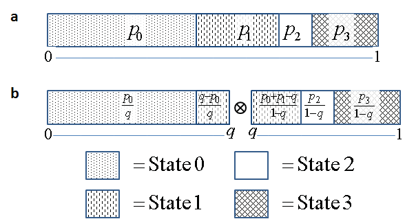
The name of the lemma comes from an intuitive representation of this equation. We can let probability distributions be represented by an interval covered with blocks. Each block corresponds to a different state of the distribution (a block can only be on the rightside of a block whose state it is greater than) and the ratio of the block length to the interval length represents the probability of the state. Then any cut along the interval will produce two separate block-intervals corresponding to exactly the distributions calculated above. This means that for any equation of this form, the block-interval cut will hold. Conversely, any cut of a block-interval corresponds to an equation with the appropriate distributions substituted. (see Figure 8).
Refer to caption
Figure 8: Block-Interval visualization (rational). We want to realize (p0,p1,p2,p3)subscript𝑝0subscript𝑝1subscript𝑝2subscript𝑝3(p_{0},p_{1},p_{2},p_{3}). A tensor-product\otimes symbol marks where the cut occurs, which corresponds to the use of one pswitch. (a) We start with one interval split into blocks corresponding to the pswitch probabilities. (b) When we cut with pswitch (q,,1q)𝑞1𝑞(q,...,1-q), the interval is separated into 2 intervals: [0,q]0𝑞[0,q] and [q,1]𝑞1[q,1].

V-A State Reduction

Given the results already proved on two state distributions, one natural way to tackle N𝑁N states is to first reduce the given N𝑁N-state distribution into compositions of 2-state distributions. Then, if algorithms already exist for those 2-state forms, we are done.

Theorem 4 (State Reduction Algorithm)

Using the switch set S ={12}absent12=\{\frac{1}{2}\}, we can reduce any N-state distribution of the form (x0q,x1q,,xN1q)subscript𝑥0𝑞subscript𝑥1𝑞subscript𝑥𝑁1𝑞(\frac{x_{0}}{q},\frac{x_{1}}{q},...,\frac{x_{N-1}}{q}) into at most N1𝑁1N-1 two-state distributions of the form (,xiq,,xjq,)subscript𝑥𝑖𝑞subscript𝑥𝑗𝑞(...,\frac{x_{i}}{q},...,\frac{x_{j}}{q},...) using at most flog2q,N=(N1)(log2qlog2N)+2log2N1subscript𝑓subscript2𝑞𝑁𝑁1subscript2𝑞subscript2𝑁superscript2subscript2𝑁1f_{\log_{2}q,N}=(N-1)(\log_{2}q-\lceil\log_{2}N\rceil)+2^{\lceil\log_{2}N\rceil}-1 switches with the following algorithm - for an example, see Figure 9a:

  if p is a 2 state distribution𝑝 is a 2 state distributionp\text{ is a 2 state distribution} then
     return p𝑝p
  else if x0q>12subscript𝑥0𝑞12\frac{x_{0}}{q}>\frac{1}{2} then
     return 12(2x0qq,2x1q,,2xN1q)122subscript𝑥0𝑞𝑞2subscript𝑥1𝑞2subscript𝑥𝑁1𝑞\frac{1}{2}(\frac{2x_{0}-q}{q},\frac{2x_{1}}{q},...,\frac{2x_{N-1}}{q})
  else if x0+x1q>12subscript𝑥0subscript𝑥1𝑞12\frac{x_{0}+x_{1}}{q}>\frac{1}{2} then
     return (2x0q,q2x0q,)+12(0,2x0+2x1qq,2x2q,)2subscript𝑥0𝑞𝑞2subscript𝑥0𝑞1202subscript𝑥02subscript𝑥1𝑞𝑞2subscript𝑥2𝑞(\frac{2x_{0}}{q},\frac{q-2x_{0}}{q},...)+\frac{1}{2}(0,\frac{2x_{0}+2x_{1}-q}{q},\frac{2x_{2}}{q},...)
  else if … then
     …
  else if x0+x1++xN1q>12subscript𝑥0subscript𝑥1subscript𝑥𝑁1𝑞12\frac{x_{0}+x_{1}+...+x_{N-1}}{q}>\frac{1}{2} then
     return (2x0q,2x1q,,2xN1qq)+122subscript𝑥0𝑞2subscript𝑥1𝑞2subscript𝑥𝑁1𝑞𝑞12(\frac{2x_{0}}{q},\frac{2x_{1}}{q},...,\frac{2x_{N-1}-q}{q})+\frac{1}{2}
  end if
Proof:

To prove this theorem, we need to show that 1) the breakdown of probabilities in each round is valid, 2) the algorithm will eventually terminate, and 3) the construction will have used flog2q,Nsubscript𝑓subscript2𝑞𝑁f_{\log_{2}q,N} pswitches, where fn,Nsubscript𝑓𝑛𝑁f_{n,N} is the complexity defined for binary N𝑁N-state distributions.

Notice that choosing q=2𝑞2q=2 gives us the exact same algorithm as the binary N𝑁N-state algorithm (except for the terminate clause). As with the binary case, Part 1 of the proof follows directly from the max-min composition rules.

We will now argue that the algorithm terminates. Let k𝑘k be the number of ‘rounds’ the algorithm takes. Using the block-interval representation, we see that after each round, any interval will either have 2absent2\leq 2 blocks (states) or the interval size will be 12k1superscript2𝑘\frac{1}{2^{k}}. Then when the interval size is less than 1q1𝑞\frac{1}{q}, each interval cannot have more than 3 blocks; otherwise, the middle block will be less than 1q1𝑞\frac{1}{q}, which is not possible except for a zero probability. Therefore, we have proved that the algorithm will eventually terminate.

To prove the complexity, we need to calculate the number of ‘rounds’ before termination of the algorithm. This will happen at,

I𝐼\displaystyle I =12k1qabsent1superscript2𝑘1𝑞\displaystyle=\frac{1}{2^{k}}\leq\frac{1}{q}
2kqabsentsuperscript2𝑘𝑞\displaystyle\implies 2^{k}\geq q
klog2qabsent𝑘subscript2𝑞\displaystyle\implies k\geq\log_{2}q

Since the algorithm is identical to the binary N𝑁N-state distribution, we can use the same complexity bound. In this case, n𝑛n corresponds to the k𝑘k-th round when the algorithm terminates. Therefore, we use at most (N1)(log2qlog2N)+2log2N1𝑁1subscript2𝑞subscript2𝑁superscript2subscript2𝑁1(N-1)(\log_{2}q-\lceil\log_{2}N\rceil)+2^{\lceil\log_{2}N\rceil}-1 pswitches. ∎

Refer to caption
Figure 9: Algorithm Illustrations. (a) An example of the state recursion algorithm. (b) An example of the denominator recursion algorithm.

V-B Denominator Reduction

The second approach to realizing rational N𝑁N-state distributions is to use a different switch set to directly reduces the power in the denominator. The intuition comes from a generalization of the block-interval construction. Rather than just cutting it at one point, i.e. at 1212\frac{1}{2} for realizing binary distributions, we can cut it at the points 1q,2q,, and q1q1𝑞2𝑞 and 𝑞1𝑞\frac{1}{q},\frac{2}{q},...,\text{ and }\frac{q-1}{q} to get q𝑞q equally sized intervals.

Theorem 5 (Denominator Reduction Algorithm)

Using S ={12,13,14,,1q}absent1213141𝑞=\{\frac{1}{2},\frac{1}{3},\frac{1}{4},...,\frac{1}{q}\} and the deterministic switches, we can realize any distribution (x0qn,x1qn,,xN1qn)subscript𝑥0superscript𝑞𝑛subscript𝑥1superscript𝑞𝑛subscript𝑥𝑁1superscript𝑞𝑛(\frac{x_{0}}{q^{n}},\frac{x_{1}}{q^{n}},...,\frac{x_{N-1}}{q^{n}}) using at most (N1)(q1)(nlogqN)+qlogqN1𝑁1𝑞1𝑛subscript𝑞𝑁superscript𝑞subscript𝑞𝑁1(N-1)(q-1)(n-\lceil\log_{q}N\rceil)+q^{\lceil\log_{q}N\rceil}-1 switches with the following algorithm - for an example, see Figure 9b:

  Define the following quantities for j=0,1,2,,q𝑗012𝑞j=0,1,2,...,q.
  kj=subscript𝑘𝑗absentk_{j}= the smallest index at which i=0kjpi>jqsuperscriptsubscript𝑖0subscript𝑘𝑗subscript𝑝𝑖𝑗𝑞\sum_{i=0}^{k_{j}}p_{i}>\frac{j}{q}
  Lj=i=0kj1xi(q1)qn1qn1subscript𝐿𝑗superscriptsubscript𝑖0subscript𝑘𝑗1subscript𝑥𝑖𝑞1superscript𝑞𝑛1superscript𝑞𝑛1L_{j}=\frac{\sum_{i=0}^{k_{j-1}}x_{i}-(q-1)q^{n-1}}{q^{n-1}}
  Rj=qn1i=0kj1xiqn1subscript𝑅𝑗superscript𝑞𝑛1superscriptsubscript𝑖0subscript𝑘𝑗1subscript𝑥𝑖superscript𝑞𝑛1R_{j}=\frac{q^{n-1}-\sum_{i=0}^{k_{j}-1}x_{i}}{q^{n-1}}
  if pS𝑝𝑆p\in S then
     return p𝑝p
  else
     return (x0qn1,,xk11qn1,R0,0,)subscript𝑥0superscript𝑞𝑛1subscript𝑥subscript𝑘11superscript𝑞𝑛1subscript𝑅00(\frac{x_{0}}{q^{n-1}},...,\frac{x_{k_{1}-1}}{q^{n-1}},R_{0},0,...)
     +12(,0,L2,xk1+1qn1,,xk21qn1,R2,0,)120subscript𝐿2subscript𝑥subscript𝑘11superscript𝑞𝑛1subscript𝑥subscript𝑘21superscript𝑞𝑛1subscript𝑅20+\frac{1}{2}(...,0,L_{2},\frac{x_{k_{1}+1}}{q^{n-1}},...,\frac{x_{k_{2}-1}}{q^{n-1}},R_{2},0,...)
     ++...
     +1q1(,0,Lq1,xkq2+1qn1,,xkq11qn1,Rq1,0,)1𝑞10subscript𝐿𝑞1subscript𝑥subscript𝑘𝑞21superscript𝑞𝑛1subscript𝑥subscript𝑘𝑞11superscript𝑞𝑛1subscript𝑅𝑞10+\frac{1}{q-1}(...,0,L_{q-1},\frac{x_{k_{q-2}+1}}{q^{n-1}},...,\frac{x_{k_{q-1}-1}}{q^{n-1}},R_{q-1},0,...)
     +1q(,0,Lq,xkq1+1qn1,,xN1qn1)1𝑞0subscript𝐿𝑞subscript𝑥subscript𝑘𝑞11superscript𝑞𝑛1subscript𝑥𝑁1superscript𝑞𝑛1+\frac{1}{q}(...,0,L_{q},\frac{x_{k_{q-1}+1}}{q^{n-1}},...,\frac{x_{N-1}}{q^{n-1}})
  end if
Proof:

The idea of the construction is to perform q1𝑞1q-1 iterations of the block-interval construction lemma for each reduction of a pswitch. WLOG, let the original interval have length 1. Then the first cut at q1q𝑞1𝑞\frac{q-1}{q} gives intervals of length q1q𝑞1𝑞\frac{q-1}{q} and 1q1𝑞\frac{1}{q}. The second cut at q2q1𝑞2𝑞1\frac{q-2}{q-1} of the q1q𝑞1𝑞\frac{q-1}{q} interval gives intervals of length q1qq2q1=q2q𝑞1𝑞𝑞2𝑞1𝑞2𝑞\frac{q-1}{q}\frac{q-2}{q-1}=\frac{q-2}{q} and q1q1q1=1q𝑞1𝑞1𝑞11𝑞\frac{q-1}{q}\frac{1}{q-1}=\frac{1}{q}. The third cut leaves an interval of length q1qq2q1q3q2=q3q𝑞1𝑞𝑞2𝑞1𝑞3𝑞2𝑞3𝑞\frac{q-1}{q}\frac{q-2}{q-1}\frac{q-3}{q-2}=\frac{q-3}{q} and another 1q1𝑞\frac{1}{q} interval. As this continues, we get q𝑞q intervals of length 1q1𝑞\frac{1}{q}. Our expression is exactly that of the block-interval construction lemma applied to the above description. Then since at each ‘round’ of these decompositions, we reduce the denominator by 1, we will eventually terminate when n=0𝑛0n=0, which is a deterministic switch.

The proof for the complexity is similar to the N𝑁N-state binary proof. If we let fq,n,Nsubscript𝑓𝑞𝑛𝑁f_{q,n,N} be the maximum number of pswitches needed, then we have the following recursive relations:

fq,n,1subscript𝑓𝑞𝑛1\displaystyle f_{q,n,1} =0absent0\displaystyle=0
fq,0,Nsubscript𝑓𝑞0𝑁\displaystyle f_{q,0,N} =0absent0\displaystyle=0
fq,n,Nsubscript𝑓𝑞𝑛𝑁\displaystyle f_{q,n,N} =maxi1,i2,,iq:jij=N+q1(q1+jfq,n1,ij)absentsubscript:subscript𝑖1subscript𝑖2subscript𝑖𝑞subscript𝑗subscript𝑖𝑗𝑁𝑞1𝑞1subscript𝑗subscript𝑓𝑞𝑛1subscript𝑖𝑗\displaystyle=\max_{i_{1},i_{2},...,i_{q}:\sum_{j}i_{j}=N+q-1}(q-1+\sum_{j}f_{q,n-1,i_{j}})

One observation to note is that for q=2𝑞2q=2, we get the same recursive functions as in the binary algorithm, which is expected:

f2,n,1subscript𝑓2𝑛1\displaystyle f_{2,n,1} =0absent0\displaystyle=0
f2,0,Nsubscript𝑓20𝑁\displaystyle f_{2,0,N} =0absent0\displaystyle=0
f2,n,Nsubscript𝑓2𝑛𝑁\displaystyle f_{2,n,N} =maxi1,i2:i1+i2=N1f2,n1,i1+f2,n1,i2+1absentsubscript:subscript𝑖1subscript𝑖2subscript𝑖1subscript𝑖2𝑁1subscript𝑓2𝑛1subscript𝑖1subscript𝑓2𝑛1subscript𝑖21\displaystyle=\max_{i_{1},i_{2}:i_{1}+i_{2}=N-1}f_{2,n-1,i_{1}}+f_{2,n-1,i_{2}}+1

To go from this recursive form to the closed form version, we use similar methods to the binary N𝑁N-state complexity function, so we will only outline the steps:

  1. 1.

    First prove that the recursive expression is maximized when all ij{N2,N2+1}subscript𝑖𝑗𝑁2𝑁21i_{j}\in\{\lceil\frac{N}{2}\rceil,\lfloor\frac{N}{2}\rfloor+1\}. This is done by showing that the closed form for fq,n,Nsubscript𝑓𝑞𝑛𝑁f_{q,n,N} has a nonincreasing discrete derivative in N𝑁N, i.e. fq,n,N+1fq,n,Nsubscript𝑓𝑞𝑛𝑁1subscript𝑓𝑞𝑛𝑁f_{q,n,N+1}-f_{q,n,N} is nonincreasing as N𝑁N increases.

  2. 2.

    Next show that the recursive expression evaluated at the appropriate ijsubscript𝑖𝑗i_{j} will achieve the closed form by breaking it up into cases to simplify the ceiling and floor expressions.

Corollary 1

Let q=p1k1p2k2pmaxkmax𝑞superscriptsubscript𝑝1subscript𝑘1superscriptsubscript𝑝2subscript𝑘2superscriptsubscript𝑝𝑚𝑎𝑥subscript𝑘𝑚𝑎𝑥q=p_{1}^{k_{1}}p_{2}^{k_{2}}...p_{max}^{k_{max}}, where pisubscript𝑝𝑖p_{i} are primes. Then using S ={12,13,14,,1pmax}absent1213141subscript𝑝𝑚𝑎𝑥=\{\frac{1}{2},\frac{1}{3},\frac{1}{4},...,\frac{1}{p_{max}}\}, we can realize any distribution (x0q,x1q,,xN1q)subscript𝑥0𝑞subscript𝑥1𝑞subscript𝑥𝑁1𝑞(\frac{x_{0}}{q},\frac{x_{1}}{q},...,\frac{x_{N-1}}{q}) using at most ifpi,ki,Nsubscript𝑖subscript𝑓subscript𝑝𝑖subscript𝑘𝑖𝑁\sum_{i}f_{p_{i},k_{i},N} pswitches.

Proof:

Here we are simply applying denominator reduction on each pikisuperscriptsubscript𝑝𝑖subscript𝑘𝑖p_{i}^{k_{i}}. The complexity is just a summation of each step. ∎

Corollary 2

Let q=p1k1p2k2pmaxkmax𝑞superscriptsubscript𝑝1subscript𝑘1superscriptsubscript𝑝2subscript𝑘2superscriptsubscript𝑝𝑚𝑎𝑥subscript𝑘𝑚𝑎𝑥q=p_{1}^{k_{1}}p_{2}^{k_{2}}...p_{max}^{k_{max}}, where pisubscript𝑝𝑖p_{i} are primes. Then using S ={12,13,15,,1pmax}absent1213151subscript𝑝𝑚𝑎𝑥=\{\frac{1}{2},\frac{1}{3},\frac{1}{5},...,\frac{1}{p_{max}}\}, we can realize any distribution (x0q,x1q,,xN1q)subscript𝑥0𝑞subscript𝑥1𝑞subscript𝑥𝑁1𝑞(\frac{x_{0}}{q},\frac{x_{1}}{q},...,\frac{x_{N-1}}{q}).

Proof:

Our claim here is that we can reduce the switch set to the inverse of the primes up to pmaxsubscript𝑝𝑚𝑎𝑥p_{max}. This is because using all of these switches, we can generate any other 1k1𝑘\frac{1}{k}, where k𝑘k is composite. However, this means that the number of pswitches will go up, i.e. 1414\frac{1}{4} will now use 2 switches 12121212\frac{1}{2}*\frac{1}{2}. We have not analyzed the complexity that this reduction in the switch set would result in. ∎

VI Robustness of Probability Generation

The above algorithms looked at probability generation given a fixed switch set of distributions. However, in physical systems, it may be the case that the generation of randomness is error-prone. If we want to use a pswitch with distribution (p0,p1)subscript𝑝0subscript𝑝1(p_{0},p_{1}), the physical pswitch may actually have distribution (p0+ϵ,p1ϵ)subscript𝑝0italic-ϵsubscript𝑝1italic-ϵ(p_{0}+\epsilon,p_{1}-\epsilon). Define the error of such a pswitch as |ϵ|italic-ϵ|\epsilon|[11]. Loh, Zhou, and Bruck looked at generating 2-state probabilities given pswitches with errors. They found that any binary distribution generated according to their algorithm, regardless of size, had error bounded by 2ϵ2italic-ϵ2\epsilon. They also showed similar bounds for different distributions.

We examine the same problem in the context of multivalued distribution generation and show that a generalized result holds for any number of states. Define the error of a multivalued distribution as the largest error over all the states. That is, if a pswitch with desired distribution (p0,p1,,pN1)subscript𝑝0subscript𝑝1subscript𝑝𝑁1(p_{0},p_{1},...,p_{N-1}) has an actual distribution of (p0+ϵ0,p1+ϵ1,,pN1+ϵN1)subscript𝑝0subscriptitalic-ϵ0subscript𝑝1subscriptitalic-ϵ1subscript𝑝𝑁1subscriptitalic-ϵ𝑁1(p_{0}+\epsilon_{0},p_{1}+\epsilon_{1},...,p_{N-1}+\epsilon_{N-1}), then the error of the switch is maxi|ϵi|subscript𝑖subscriptitalic-ϵ𝑖\max_{i}|\epsilon_{i}|.

We will begin by demonstrating robustness for N𝑁N-state binary distributions generated according to the algorithm in section IV. This algorithm uses switches from the switch set S ={12}absent12=\{\frac{1}{2}\} as well as the deterministic switches. For our analysis, we allow errors on the active states of pswitches. As a result, deterministic switches have no errors since the sum of the single active probability must equal 1. The 1212\frac{1}{2}-pswitch has distribution (12+ϵ^,0,,0,12ϵ^)12^italic-ϵ0012^italic-ϵ(\frac{1}{2}+\hat{\epsilon},0,...,0,\frac{1}{2}-\hat{\epsilon}), |ϵ^|ϵ^italic-ϵitalic-ϵ|\hat{\epsilon}|\leq\epsilon.

Lemma 4 (Error Bound on Boundary States)

Generate any distribution (,0,xi2n,,xj2n,0,)0subscript𝑥𝑖superscript2𝑛subscript𝑥𝑗superscript2𝑛0(...,0,\frac{x_{i}}{2^{n}},...,\frac{x_{j}}{2^{n}},0,...) according to the binary N𝑁N-state algorithm where state i𝑖i is the smallest active state and state j𝑗j is the largest active state. If we allow at most ϵitalic-ϵ\epsilon error on the pswitches in the switch set, then the actual distribution generated will be (,0,xi2n+δi,,xj2n+δj,0,)0subscript𝑥𝑖superscript2𝑛subscript𝛿𝑖subscript𝑥𝑗superscript2𝑛subscript𝛿𝑗0(...,0,\frac{x_{i}}{2^{n}}+\delta_{i},...,\frac{x_{j}}{2^{n}}+\delta_{j},0,...) where |δi|2ϵsubscript𝛿𝑖2italic-ϵ|\delta_{i}|\leq 2\epsilon, |δj|2ϵsubscript𝛿𝑗2italic-ϵ|\delta_{j}|\leq 2\epsilon.

Proof:

In each step of the algorithm, a distribution r=(,ri,,rj,)𝑟subscript𝑟𝑖subscript𝑟𝑗r=(...,r_{i},...,r_{j},...) is made out of 2 pswitches p=(,pi,,pk,)𝑝subscript𝑝𝑖subscript𝑝𝑘p=(...,p_{i},...,p_{k},...) and q=(,qk,,qj,)𝑞subscript𝑞𝑘subscript𝑞𝑗q=(...,q_{k},...,q_{j},...) where ijk𝑖𝑗𝑘i\leq j\leq k. The composition is in the form r=p+(12,,12)q𝑟𝑝1212𝑞r=p+(\frac{1}{2},...,\frac{1}{2})q. We will prove robustness using induction on switches p𝑝p and q𝑞q.

Base Case: We use the deterministic switches as our base case switches (for these, i=k𝑖𝑘i=k or k=j𝑘𝑗k=j). These trivially satisfy the induction hypothesis since they have no error.

Inductive Step: Assume we are given p𝑝p and q𝑞q satisfying the inductive hypothesis. That is, for p=(,pi+Δi,,pk+Δk,)𝑝subscript𝑝𝑖subscriptΔ𝑖subscript𝑝𝑘subscriptΔ𝑘p=(...,p_{i}+\Delta_{i},...,p_{k}+\Delta_{k},...), q=(,qk+δk,,qj+δj,)𝑞subscript𝑞𝑘subscript𝛿𝑘subscript𝑞𝑗subscript𝛿𝑗q=(...,q_{k}+\delta_{k},...,q_{j}+\delta_{j},...), |Δi|,|Δk|,|δk|,|δj|2ϵsubscriptΔ𝑖subscriptΔ𝑘subscript𝛿𝑘subscript𝛿𝑗2italic-ϵ|\Delta_{i}|,|\Delta_{k}|,|\delta_{k}|,|\delta_{j}|\leq 2\epsilon. Then the errors for states i𝑖i and j𝑗j on distribution r=p+(12+ϵ^,,12ϵ^)q𝑟𝑝12^italic-ϵ12^italic-ϵ𝑞r=p+(\frac{1}{2}+\hat{\epsilon},...,\frac{1}{2}-\hat{\epsilon})q can be calculated as follows:

|errori<k|subscripterror𝑖𝑘\displaystyle|\text{error}_{i<k}| =|(12+ϵ^)(pi+Δi)12pi|absent12^italic-ϵsubscript𝑝𝑖subscriptΔ𝑖12subscript𝑝𝑖\displaystyle=|(\frac{1}{2}+\hat{\epsilon})(p_{i}+\Delta_{i})-\frac{1}{2}p_{i}|
=|12Δi+ϵ^(pi+Δi)|absent12subscriptΔ𝑖^italic-ϵsubscript𝑝𝑖subscriptΔ𝑖\displaystyle=|\frac{1}{2}\Delta_{i}+\hat{\epsilon}(p_{i}+\Delta_{i})|
12|Δi|+|ϵ^||pi+Δi|absent12subscriptΔ𝑖^italic-ϵsubscript𝑝𝑖subscriptΔ𝑖\displaystyle\leq\frac{1}{2}|\Delta_{i}|+|\hat{\epsilon}||p_{i}+\Delta_{i}|
2ϵabsent2italic-ϵ\displaystyle\leq 2\epsilon
|errori=k|subscripterror𝑖𝑘\displaystyle|\text{error}_{i=k}| =|(12+ϵ^)+(12ϵ^)(qi+δi)(12+12qi)|absent12^italic-ϵ12^italic-ϵsubscript𝑞𝑖subscript𝛿𝑖1212subscript𝑞𝑖\displaystyle=|(\frac{1}{2}+\hat{\epsilon})+(\frac{1}{2}-\hat{\epsilon})(q_{i}+\delta_{i})-(\frac{1}{2}+\frac{1}{2}q_{i})|
=|12δi+ϵ^(1(qi+δi))|absent12subscript𝛿𝑖^italic-ϵ1subscript𝑞𝑖subscript𝛿𝑖\displaystyle=|\frac{1}{2}\delta_{i}+\hat{\epsilon}(1-(q_{i}+\delta_{i}))|
12|δi|+|ϵ^||1(qi+δi)|absent12subscript𝛿𝑖^italic-ϵ1subscript𝑞𝑖subscript𝛿𝑖\displaystyle\leq\frac{1}{2}|\delta_{i}|+|\hat{\epsilon}||1-(q_{i}+\delta_{i})|
2ϵabsent2italic-ϵ\displaystyle\leq 2\epsilon
|errorj>k|subscripterror𝑗𝑘\displaystyle|\text{error}_{j>k}| =|(12ϵ^)(qj+δj)12qj|absent12^italic-ϵsubscript𝑞𝑗subscript𝛿𝑗12subscript𝑞𝑗\displaystyle=|(\frac{1}{2}-\hat{\epsilon})(q_{j}+\delta_{j})-\frac{1}{2}q_{j}|
=|12δj+ϵ^(qj+δj)|absent12subscript𝛿𝑗^italic-ϵsubscript𝑞𝑗subscript𝛿𝑗\displaystyle=|\frac{1}{2}\delta_{j}+\hat{\epsilon}(q_{j}+\delta_{j})|
12|δj|+|ϵ^||qj+δj|absent12subscript𝛿𝑗^italic-ϵsubscript𝑞𝑗subscript𝛿𝑗\displaystyle\leq\frac{1}{2}|\delta_{j}|+|\hat{\epsilon}||q_{j}+\delta_{j}|
2ϵabsent2italic-ϵ\displaystyle\leq 2\epsilon
|errorj=k|subscripterror𝑗𝑘\displaystyle|\text{error}_{j=k}| =|(12ϵ^)+(12+ϵ^)(pj+Δj)(12+12pj)|absent12^italic-ϵ12^italic-ϵsubscript𝑝𝑗subscriptΔ𝑗1212subscript𝑝𝑗\displaystyle=|(\frac{1}{2}-\hat{\epsilon})+(\frac{1}{2}+\hat{\epsilon})(p_{j}+\Delta_{j})-(\frac{1}{2}+\frac{1}{2}p_{j})|
=|12Δj+ϵ^(1(pj+Δj))|absent12subscriptΔ𝑗^italic-ϵ1subscript𝑝𝑗subscriptΔ𝑗\displaystyle=|\frac{1}{2}\Delta_{j}+\hat{\epsilon}(1-(p_{j}+\Delta_{j}))|
12|Δj|+|ϵ^||1(pj+Δj)|absent12subscriptΔ𝑗^italic-ϵ1subscript𝑝𝑗subscriptΔ𝑗\displaystyle\leq\frac{1}{2}|\Delta_{j}|+|\hat{\epsilon}||1-(p_{j}+\Delta_{j})|
2ϵabsent2italic-ϵ\displaystyle\leq 2\epsilon

Then we find that the errors for states i𝑖i and j𝑗j still satisfy the inductive hypothesis, so we are done. ∎

Theorem 6 (Robustness of Binary N-state Distributions)

Generate any distribution (x02n,x12n,,xN12n)subscript𝑥0superscript2𝑛subscript𝑥1superscript2𝑛subscript𝑥𝑁1superscript2𝑛(\frac{x_{0}}{2^{n}},\frac{x_{1}}{2^{n}},...,\frac{x_{N-1}}{2^{n}}) according to the binary N𝑁N-state algorithm. If we allow the pswitches in the switch set S =12absent12=\frac{1}{2} to have up to ϵitalic-ϵ\epsilon error in the active states, then the actual distribution (x02n+δ0,x12n+δ1,,xN12n+δN1)subscript𝑥0superscript2𝑛subscript𝛿0subscript𝑥1superscript2𝑛subscript𝛿1subscript𝑥𝑁1superscript2𝑛subscript𝛿𝑁1(\frac{x_{0}}{2^{n}}+\delta_{0},\frac{x_{1}}{2^{n}}+\delta_{1},...,\frac{x_{N-1}}{2^{n}}+\delta_{N-1}) has errors |δi|3ϵsubscript𝛿𝑖3italic-ϵ|\delta_{i}|\leq 3\epsilon, |δ0|,|δN1|2ϵsubscript𝛿0subscript𝛿𝑁12italic-ϵ|\delta_{0}|,|\delta_{N-1}|\leq 2\epsilon.

Proof:

In each step of the binary N𝑁N-state algorithm, a distribution r=(,ri,,rj,)𝑟subscript𝑟𝑖subscript𝑟𝑗r=(...,r_{i},...,r_{j},...) is made out of 2 pswitches p=(,pi,,pk,)𝑝subscript𝑝𝑖subscript𝑝𝑘p=(...,p_{i},...,p_{k},...) and q=(,qk,,qj,)𝑞subscript𝑞𝑘subscript𝑞𝑗q=(...,q_{k},...,q_{j},...) where ijk𝑖𝑗𝑘i\leq j\leq k, i𝑖i is the smallest active state and j𝑗j is the largest active state. The composition is in the form r=p+(12,,12)q𝑟𝑝1212𝑞r=p+(\frac{1}{2},...,\frac{1}{2})q. We will prove robustness using induction on switches p𝑝p and q𝑞q.

Base Case: We use the deterministic switches as our base case switches. These trivially satisfy the induction hypothesis since they have no error.

Inductive Step: Assume we are given p𝑝p and q𝑞q satisfying the inductive hypothesis. That is, for p=(,pi+Δi,,pk+Δk,)𝑝subscript𝑝𝑖subscriptΔ𝑖subscript𝑝𝑘subscriptΔ𝑘p=(...,p_{i}+\Delta_{i},...,p_{k}+\Delta_{k},...), q=(,qk+δk,,qj+δj,)𝑞subscript𝑞𝑘subscript𝛿𝑘subscript𝑞𝑗subscript𝛿𝑗q=(...,q_{k}+\delta_{k},...,q_{j}+\delta_{j},...), |Δs|,|δs|3ϵsubscriptΔ𝑠subscript𝛿𝑠3italic-ϵ|\Delta_{s}|,|\delta_{s}|\leq 3\epsilon, |Δi|,|Δk|,|δk|,|δj|2ϵsubscriptΔ𝑖subscriptΔ𝑘subscript𝛿𝑘subscript𝛿𝑗2italic-ϵ|\Delta_{i}|,|\Delta_{k}|,|\delta_{k}|,|\delta_{j}|\leq 2\epsilon. Then the errors for states s𝑠s on distribution r=p+(12+ϵ^,,12ϵ^)q𝑟𝑝12^italic-ϵ12^italic-ϵ𝑞r=p+(\frac{1}{2}+\hat{\epsilon},...,\frac{1}{2}-\hat{\epsilon})q can be calculated as follows:

  1. 1.

    For s=i,j𝑠𝑖𝑗s=i,j, we apply the previous lemma on boundary states

  2. 2.

    For i<s<k,k<s<jformulae-sequence𝑖𝑠𝑘𝑘𝑠𝑗i<s<k,k<s<j, we have a similar expression as calculated in the proof for boundary error (steps skipped below since shown earlier).

    |errori<s<k|subscripterror𝑖𝑠𝑘\displaystyle|\text{error}_{i<s<k}| 12|Δs|+|ϵ^||ps+Δs|absent12subscriptΔ𝑠^italic-ϵsubscript𝑝𝑠subscriptΔ𝑠\displaystyle\leq\frac{1}{2}|\Delta_{s}|+|\hat{\epsilon}||p_{s}+\Delta_{s}|
    52ϵ3ϵabsent52italic-ϵ3italic-ϵ\displaystyle\leq\frac{5}{2}\epsilon\leq 3\epsilon
    |errork<s<j|subscripterror𝑘𝑠𝑗\displaystyle|\text{error}_{k<s<j}| 12|δs|+|ϵ^||qs+δs|absent12subscript𝛿𝑠^italic-ϵsubscript𝑞𝑠subscript𝛿𝑠\displaystyle\leq\frac{1}{2}|\delta_{s}|+|\hat{\epsilon}||q_{s}+\delta_{s}|
    52ϵ3ϵabsent52italic-ϵ3italic-ϵ\displaystyle\leq\frac{5}{2}\epsilon\leq 3\epsilon
  3. 3.

    For s=k𝑠𝑘s=k, we have the following error:

    |errors=k|subscripterror𝑠𝑘\displaystyle|\text{error}_{s=k}| =|(12+ϵ^)(pk+Δk)+(12ϵ^)(qk+δk)\displaystyle=|(\frac{1}{2}+\hat{\epsilon})(p_{k}+\Delta_{k})+(\frac{1}{2}-\hat{\epsilon})(q_{k}+\delta_{k})
    12(pk+qk)|\displaystyle\ \ \ -\frac{1}{2}(p_{k}+q_{k})|
    =|12Δk+12δk+ϵ^[(pk+Δk)(qk+δk)]|absent12subscriptΔ𝑘12subscript𝛿𝑘^italic-ϵdelimited-[]subscript𝑝𝑘subscriptΔ𝑘subscript𝑞𝑘subscript𝛿𝑘\displaystyle=|\frac{1}{2}\Delta_{k}+\frac{1}{2}\delta_{k}+\hat{\epsilon}[(p_{k}+\Delta_{k})-(q_{k}+\delta_{k})]|
    12(|Δk|+|δk|)+ϵabsent12subscriptΔ𝑘subscript𝛿𝑘italic-ϵ\displaystyle\leq\frac{1}{2}(|\Delta_{k}|+|\delta_{k}|)+\epsilon
    3ϵabsent3italic-ϵ\displaystyle\leq 3\epsilon

Then we find that the errors for all states s𝑠s still satisfy the inductive hypothesis, so for i=0𝑖0i=0 and j=N1𝑗𝑁1j=N-1, we are done. ∎

Now we will show that the N𝑁N-state rational distributions generated according to the algorithms in Section V are also robust. For the state reduction algorithm, all the results are identical to the binary robustness results since the proofs did not assume that p𝑝p and q𝑞q were binary distributions. However, since the state reduction algorithm depends on other unknown 2-state algorithms, the error will depend on the errors generated from the 2-state algorithm. The robustness result for the denominator reduction algorithm is very similar to the one for binary distributions. The main difference is that we have a different switch set S ={12,13,,1q}absent12131𝑞=\{\frac{1}{2},\frac{1}{3},...,\frac{1}{q}\}.

Theorem 7 (Robustness of Rational Distributions)

Generate any distribution (x0qn,x1qn,,xN1qn)subscript𝑥0superscript𝑞𝑛subscript𝑥1superscript𝑞𝑛subscript𝑥𝑁1superscript𝑞𝑛(\frac{x_{0}}{q^{n}},\frac{x_{1}}{q^{n}},...,\frac{x_{N-1}}{q^{n}}) according to the denominator reduction algorithm. If we allow the pswitches in the switch set S ={12,,1q}absent121𝑞=\{\frac{1}{2},...,\frac{1}{q}\} to have up to ϵitalic-ϵ\epsilon error in the active states, then the actual distribution (x0qn+δ0,x1qn+δ1,,xN1qn+δN1)subscript𝑥0superscript𝑞𝑛subscript𝛿0subscript𝑥1superscript𝑞𝑛subscript𝛿1subscript𝑥𝑁1superscript𝑞𝑛subscript𝛿𝑁1(\frac{x_{0}}{q^{n}}+\delta_{0},\frac{x_{1}}{q^{n}}+\delta_{1},...,\frac{x_{N-1}}{q^{n}}+\delta_{N-1}) has errors |δi|(q+1)ϵsubscript𝛿𝑖𝑞1italic-ϵ|\delta_{i}|\leq(q+1)\epsilon, |δ0|,|δN1|qϵsubscript𝛿0subscript𝛿𝑁1𝑞italic-ϵ|\delta_{0}|,|\delta_{N-1}|\leq q\epsilon.

Proof:

For generating rational distributions, each iteration repeats compositions of the form:

(z0,,zN1)subscript𝑧0subscript𝑧𝑁1\displaystyle(z_{0},...,z_{N-1}) =(p0,,pi1,0,)absentsubscript𝑝0subscript𝑝subscript𝑖10\displaystyle=(p_{0},...,p_{i_{1}},0,...)
+12(,0,qi1,,qi2,0,)120subscript𝑞subscript𝑖1subscript𝑞subscript𝑖20\displaystyle+\frac{1}{2}(...,0,q_{i_{1}},...,q_{i_{2}},0,...)
+13(,0,ri2,,ri3,0,)130subscript𝑟subscript𝑖2subscript𝑟subscript𝑖30\displaystyle+\frac{1}{3}(...,0,r_{i_{2}},...,r_{i_{3}},0,...)
+\displaystyle+...
+1q(,0,yiq1,,yiq,0,)1𝑞0subscript𝑦subscript𝑖𝑞1subscript𝑦subscript𝑖𝑞0\displaystyle+\frac{1}{q}(...,0,y_{i_{q-1}},...,y_{i_{q}},0,...)

We notice that each composition of this form is the same as q1𝑞1q-1 compositions of the form (,pi,,pk,)+1q^(,qk,,qj,)subscript𝑝𝑖subscript𝑝𝑘1^𝑞subscript𝑞𝑘subscript𝑞𝑗(...,p_{i},...,p_{k},...)+\frac{1}{\hat{q}}(...,q_{k},...,q_{j},...) where q^=2,3,q^𝑞23𝑞\hat{q}=2,3,...q. Then from here, the work is almost identical to the proof of the binary distributions, so we will only outline the steps.

  1. 1.

    Prove that the boundary states of distributions formed from (,pi,,pk,)+1q^(,qk,,qj,)subscript𝑝𝑖subscript𝑝𝑘1^𝑞subscript𝑞𝑘subscript𝑞𝑗(...,p_{i},...,p_{k},...)+\frac{1}{\hat{q}}(...,q_{k},...,q_{j},...) compositions, q^{2,3,,q}^𝑞23𝑞\hat{q}\in\{2,3,...,q\} have error of at most qϵ𝑞italic-ϵq\epsilon regardless of the number of compositions (use induction). As before, we allow pswitches (q^1q^+ϵ^,,1q^ϵ^)^𝑞1^𝑞^italic-ϵ1^𝑞^italic-ϵ(\frac{\hat{q}-1}{\hat{q}}+\hat{\epsilon},...,\frac{1}{\hat{q}}-\hat{\epsilon}) to have error ϵ^ϵ^italic-ϵitalic-ϵ\hat{\epsilon}\leq\epsilon.

  2. 2.

    Using the boundary state error, prove that the errors of all states have error of at most (q1)ϵ𝑞1italic-ϵ(q-1)\epsilon.

Then, since all the compositions making up the rational distributions are of the form (,pi,,pk,)+1q^(,qk,,qj,)subscript𝑝𝑖subscript𝑝𝑘1^𝑞subscript𝑞𝑘subscript𝑞𝑗(...,p_{i},...,p_{k},...)+\frac{1}{\hat{q}}(...,q_{k},...,q_{j},...), the steps above are sufficient for proving our theorem. ∎

VII Universal Probability Generator

Up till now, we have only looked at circuits with set switches and described algorithms for realizing specific probability distributions. A next question is: What about circuits that implement stochastic functions? That is, how can we reason about circuits that implement different probability distributions given ‘input’ switches? Wilhelm and Bruck approached this problem for the 2-state version[9] by constructing a circuit which they called a Universal Probability Generator (UPG). The function of this circuit was to map n𝑛n-deterministic bits into output probabilities of the form x02nsubscript𝑥0superscript2𝑛\frac{x_{0}}{2^{n}} in increasing order.

This functionality alone is not surprising since it can easily be done with an exponential number of switches using a tree-like structure; however, the remarkable result is that the UPG only requires a linear number of switches in n𝑛n. In this section we will show a generalization of this circuit which is able to realize any binary probability distribution of the form (x02n,x12n,,xN12n)subscript𝑥0superscript2𝑛subscript𝑥1superscript2𝑛subscript𝑥𝑁1superscript2𝑛(\frac{x_{0}}{2^{n}},\frac{x_{1}}{2^{n}},...,\frac{x_{N-1}}{2^{n}}) using a number of switches that is polynomial in n𝑛n with degree N1𝑁1N-1.

The strategy we will take for deriving the UPG construction is first to ask: ‘How should the UPG function?’ Then we will build a circuit that naively implements the functionality and use algebraic rules to reduce the complexity of the circuit.

VII-A 2-state UPG

We will first review the 2-state UPG of Wilhelm and Bruck[9], deriving the results in a manner that is similar to the steps we take to get the generalized N𝑁N-state UPG.

Refer to caption
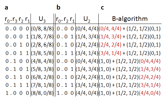
Figure 10: 2-state Universal Probability Generator (UPG) mappings (a) A mapping for a UPG that generates distributions of the form (x08,x18)subscript𝑥08subscript𝑥18(\frac{x_{0}}{8},\frac{x_{1}}{8}). (b) Removing r3subscript𝑟3r_{3}, we look at the inputs to a UPG that generates distributions of the form (x04,x14)subscript𝑥04subscript𝑥14(\frac{x_{0}}{4},\frac{x_{1}}{4}). (c) Notice that the B-algorithm decompositions of the probabilities of part (a) correspond to those in part (b).

Definition: (2-state UPG). A 2-state UPG Unsubscript𝑈𝑛U_{n} is a circuit that realizes distributions of the form (x02n,x12n)subscript𝑥0superscript2𝑛subscript𝑥1superscript2𝑛(\frac{x_{0}}{2^{n}},\frac{x_{1}}{2^{n}}) using n+1𝑛1n+1 input bits which we will refer to as r0subscript𝑟0r_{0}, r1subscript𝑟1r_{1}, …, rnsubscript𝑟𝑛r_{n}. When the input bits, in the order r0,rn,rn1,subscript𝑟0subscript𝑟𝑛subscript𝑟𝑛1r_{0},r_{n},r_{n-1}, …, r2,r1subscript𝑟2subscript𝑟1r_{2},r_{1} are set to the binary representation of x02nsubscript𝑥0superscript2𝑛\frac{x_{0}}{2^{n}}, then the circuit Unsubscript𝑈𝑛U_{n} will realize distribution (x02n,x12n)subscript𝑥0superscript2𝑛subscript𝑥1superscript2𝑛(\frac{x_{0}}{2^{n}},\frac{x_{1}}{2^{n}}). In other words, to realize any desired binary probability (x02n,x12n)subscript𝑥0superscript2𝑛subscript𝑥1superscript2𝑛(\frac{x_{0}}{2^{n}},\frac{x_{1}}{2^{n}}), we set the input bits to the state 0 probability.

As an example, we look at the input-output mappings for the circuit U3subscript𝑈3U_{3}. If we input 𝐫=0001𝐫0001\mathbf{r}=0001, the circuit will realize (18,78)1878(\frac{1}{8},\frac{7}{8}) since 18=0.001218subscript0.0012\frac{1}{8}=0.001_{2}. The input 010101010101 will realize (58,38)5838(\frac{5}{8},\frac{3}{8}) since 58=0.101258subscript0.1012\frac{5}{8}=0.101_{2} (see Figure 10a).

The motivation for the UPG circuit comes from an interesting property in the truth table. For example, let us enumerate all the outputs for U3subscript𝑈3U_{3} (Fig. 10a). For each row (input), we ask the following questions: What would the output of U2subscript𝑈2U_{2} be given the inputs r0,r2,r1subscript𝑟0subscript𝑟2subscript𝑟1r_{0},r_{2},r_{1} that were used for U3subscript𝑈3U_{3}? Is there a relationship to the construction of the U3subscript𝑈3U_{3} output probability?

If we calculate these outputs, we find that they are the same probability distributions used in the binary algorithm for 2-states (Fig. 10bc). From here, the (exponential) recursive construction is straightforward.
Refer to caption
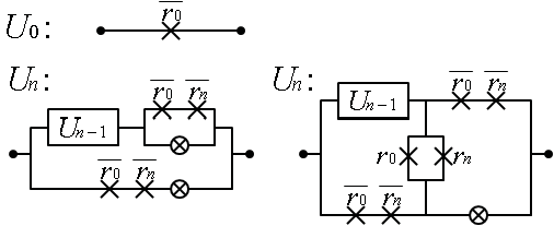
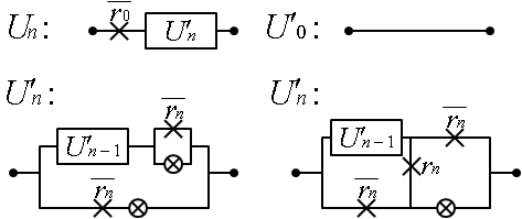
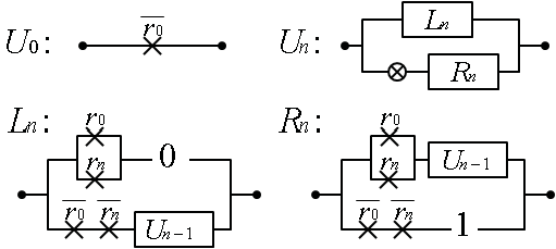
Figure 11: 2-state exponential UPG This is a UPG derived directly from the B-algorithm. It uses an exponential number of switches since Unsubscript𝑈𝑛U_{n} uses two copies of Un1subscript𝑈𝑛1U_{n-1} in its recursive construction.
Lemma 5

A 2-state UPG Unsubscript𝑈𝑛U_{n} with inputs r0,rn,,r2,r1subscript𝑟0subscript𝑟𝑛subscript𝑟2subscript𝑟1r_{0},r_{n},\ldots,r_{2},r_{1} can be constructed with an exponential number of switches using the recursive construction in Figure 11, where the n𝑛n bits used in Un1subscript𝑈𝑛1U_{n-1} are r0,rn1,,r2,r1subscript𝑟0subscript𝑟𝑛1subscript𝑟2subscript𝑟1r_{0},r_{n-1},\ldots,r_{2},r_{1}.

Proof:

We can prove this inductively.

Base Case: U0=r¯0subscript𝑈0subscript¯𝑟0U_{0}=\bar{r}_{0} realizes (0,1)01(0,1) and (1,0)10(1,0) when r0=0subscript𝑟00r_{0}=0 and r0=1subscript𝑟01r_{0}=1 respectively.

Inductive Step: Let r0n=r0+rnsubscript𝑟0𝑛subscript𝑟0subscript𝑟𝑛r_{0n}=r_{0}+r_{n}, which also implies r¯0n=r¯0r¯nsubscript¯𝑟0𝑛subscript¯𝑟0subscript¯𝑟𝑛\bar{r}_{0n}=\bar{r}_{0}\bar{r}_{n}. Assume Un1subscript𝑈𝑛1U_{n-1} realizes the correct distributions given the defined inputs. Then we want to show that

Unsubscript𝑈𝑛\displaystyle U_{n} =Ln+(12,12)Rn,absentsubscript𝐿𝑛1212subscript𝑅𝑛\displaystyle=L_{n}+(\frac{1}{2},\frac{1}{2})R_{n},
Lnsubscript𝐿𝑛\displaystyle L_{n} =r0n0+r¯0nUn1,absentsubscript𝑟0𝑛0subscript¯𝑟0𝑛subscript𝑈𝑛1\displaystyle=r_{0n}\cdot 0+\bar{r}_{0n}U_{n-1},
Rnsubscript𝑅𝑛\displaystyle R_{n} =r0nUn1+r¯0n1,absentsubscript𝑟0𝑛subscript𝑈𝑛1subscript¯𝑟0𝑛1\displaystyle=r_{0n}U_{n-1}+\bar{r}_{0n}\cdot 1,

This is equivalent to showing,

Unsubscript𝑈𝑛\displaystyle U_{n} =Ln+(12,12)Rn,absentsubscript𝐿𝑛1212subscript𝑅𝑛\displaystyle=L_{n}+(\frac{1}{2},\frac{1}{2})R_{n},
Lnsubscript𝐿𝑛\displaystyle L_{n} ={(1,0), if r0n=1Un1, if r¯0n=1absentcases10 if subscript𝑟0𝑛1subscript𝑈𝑛1 if subscript¯𝑟0𝑛1\displaystyle=\begin{cases}(1,0),&\text{ if }r_{0n}=1\\ U_{n-1},&\text{ if }\bar{r}_{0n}=1\end{cases}
Rnsubscript𝑅𝑛\displaystyle R_{n} ={Un1, if r0n=1(0,1), if r¯0n=1absentcasessubscript𝑈𝑛1 if subscript𝑟0𝑛101 if subscript¯𝑟0𝑛1\displaystyle=\begin{cases}U_{n-1},&\text{ if }r_{0n}=1\\ (0,1),&\text{ if }\bar{r}_{0n}=1\end{cases}

which is equivalent to showing,

Unsubscript𝑈𝑛\displaystyle U_{n} ={(1,0)+(12,12)Un1, if r0n=1Un1+(12,12)(0,1), if r¯0n=1absentcases101212subscript𝑈𝑛1 if subscript𝑟0𝑛1subscript𝑈𝑛1121201 if subscript¯𝑟0𝑛1\displaystyle=\begin{cases}(1,0)+(\frac{1}{2},\frac{1}{2})U_{n-1},&\text{ if }r_{0n}=1\\ U_{n-1}+(\frac{1}{2},\frac{1}{2})(0,1),&\text{ if }\bar{r}_{0n}=1\end{cases}

Here, we are reminded of the B-algorithm (for realizing any 2-state binary distribution):

(x02n,x12n)subscript𝑥0superscript2𝑛subscript𝑥1superscript2𝑛\displaystyle(\frac{x_{0}}{2^{n}},\frac{x_{1}}{2^{n}}) ={(1,0)+(12,12)(x02n11,x12n1), if x02n12(x02n1,x12n11)+(12,12)(0,1), if x02n<12absentcases101212subscript𝑥0superscript2𝑛11subscript𝑥1superscript2𝑛1 if subscript𝑥0superscript2𝑛12subscript𝑥0superscript2𝑛1subscript𝑥1superscript2𝑛11121201 if subscript𝑥0superscript2𝑛12\displaystyle=\begin{cases}(1,0)+(\frac{1}{2},\frac{1}{2})(\frac{x_{0}}{2^{n-1}}-1,\frac{x_{1}}{2^{n-1}}),&\text{ if }\frac{x_{0}}{2^{n}}\geq\frac{1}{2}\\ (\frac{x_{0}}{2^{n-1}},\frac{x_{1}}{2^{n-1}}-1)+(\frac{1}{2},\frac{1}{2})(0,1),&\text{ if }\frac{x_{0}}{2^{n}}<\frac{1}{2}\end{cases}

Then we are almost done with our proof. We know that r0n=1x02n12iffsubscript𝑟0𝑛1subscript𝑥0superscript2𝑛12r_{0n}=1\iff\frac{x_{0}}{2^{n}}\geq\frac{1}{2} and r¯0n=1x02n<12iffsubscript¯𝑟0𝑛1subscript𝑥0superscript2𝑛12\bar{r}_{0n}=1\iff\frac{x_{0}}{2^{n}}<\frac{1}{2}. In addition, if 𝐫𝐫\mathbf{r} is set to generate (x02n,x12n)subscript𝑥0superscript2𝑛subscript𝑥1superscript2𝑛(\frac{x_{0}}{2^{n}},\frac{x_{1}}{2^{n}}), then using r0,rn1,,r2,r1subscript𝑟0subscript𝑟𝑛1subscript𝑟2subscript𝑟1r_{0},r_{n-1},...,r_{2},r_{1} as inputs to Un1subscript𝑈𝑛1U_{n-1}, we get

Un1subscript𝑈𝑛1\displaystyle U_{n-1} ={(x02n11,x12n1), if r0n=1(x02n1,x12n11), if r¯0n=1absentcasessubscript𝑥0superscript2𝑛11subscript𝑥1superscript2𝑛1 if subscript𝑟0𝑛1subscript𝑥0superscript2𝑛1subscript𝑥1superscript2𝑛11 if subscript¯𝑟0𝑛1\displaystyle=\begin{cases}(\frac{x_{0}}{2^{n-1}}-1,\frac{x_{1}}{2^{n-1}}),&\text{ if }r_{0n}=1\\ (\frac{x_{0}}{2^{n-1}},\frac{x_{1}}{2^{n-1}}-1),&\text{ if }\bar{r}_{0n}=1\end{cases}

This is because when r0=0subscript𝑟00r_{0}=0, removing rnsubscript𝑟𝑛r_{n} is like shifting the fractional bits left (multiplying by 2) and then subtracting 1 if the bit removed was 1. When r0=1subscript𝑟01r_{0}=1, then removing rnsubscript𝑟𝑛r_{n} doesn’t change anything, which still satisfies 1=1(2)111211=1(2)-1. At this point, we can invoke the B-algorithm to conclude that Unsubscript𝑈𝑛U_{n} will successfully realize (x02n,x12n)subscript𝑥0superscript2𝑛subscript𝑥1superscript2𝑛(\frac{x_{0}}{2^{n}},\frac{x_{1}}{2^{n}}). ∎

Refer to caption
Figure 12: 2-state UPG reduced After reducing the exponential UPG, we get two linear UPGs. One is a sp-circuit and uses 2 stochastic switches. The other is non-sp and uses 1 stochastic switch.
Lemma 6

A 2-state UPG Unsubscript𝑈𝑛U_{n} with inputs r0,rn,,r2,r1subscript𝑟0subscript𝑟𝑛subscript𝑟2subscript𝑟1r_{0},r_{n},\ldots,r_{2},r_{1} can be constructed with a linear number of switches using either of the two recursive constructions in Figure 12, where the n𝑛n bits used in Un1subscript𝑈𝑛1U_{n-1} are r0,rn1,,r2,r1subscript𝑟0subscript𝑟𝑛1subscript𝑟2subscript𝑟1r_{0},r_{n-1},\ldots,r_{2},r_{1}.

Proof:

We will prove this by algebraically reducing the exponential UPG. Let pi=(12,12)subscript𝑝𝑖1212p_{i}=(\frac{1}{2},\frac{1}{2}) be i.i.d.

Unsubscript𝑈𝑛\displaystyle U_{n} =Ln+pnRnabsentsubscript𝐿𝑛subscript𝑝𝑛subscript𝑅𝑛\displaystyle=L_{n}+p_{n}R_{n}
=r0n0+r¯0nUn1+pn(r0nUn1+r¯0n1)absentsubscript𝑟0𝑛0subscript¯𝑟0𝑛subscript𝑈𝑛1subscript𝑝𝑛subscript𝑟0𝑛subscript𝑈𝑛1subscript¯𝑟0𝑛1\displaystyle=r_{0n}\cdot 0+\bar{r}_{0n}U_{n-1}+p_{n}(r_{0n}U_{n-1}+\bar{r}_{0n}\cdot 1)
=r¯0nUn1+pn(r0nUn1+r¯0n)absentsubscript¯𝑟0𝑛subscript𝑈𝑛1subscript𝑝𝑛subscript𝑟0𝑛subscript𝑈𝑛1subscript¯𝑟0𝑛\displaystyle=\bar{r}_{0n}U_{n-1}+p_{n}(r_{0n}U_{n-1}+\bar{r}_{0n})
=Un1(r¯0n+r0npn)+r¯0npnabsentsubscript𝑈𝑛1subscript¯𝑟0𝑛subscript𝑟0𝑛subscript𝑝𝑛subscript¯𝑟0𝑛subscript𝑝𝑛\displaystyle=U_{n-1}(\bar{r}_{0n}+r_{0n}p_{n})+\bar{r}_{0n}p_{n}
=Un1(r¯0n+pn)+r¯0npnabsentsubscript𝑈𝑛1subscript¯𝑟0𝑛subscript𝑝𝑛subscript¯𝑟0𝑛subscript𝑝𝑛\displaystyle=U_{n-1}(\bar{r}_{0n}+p_{n})+\bar{r}_{0n}p_{n}

This is exactly the form of the series parallel construction in Fig. 12

Unsubscript𝑈𝑛\displaystyle U_{n} =Ln+pnRnabsentsubscript𝐿𝑛subscript𝑝𝑛subscript𝑅𝑛\displaystyle=L_{n}+p_{n}R_{n}
=r0n0+r¯0nUn1+pn(r0nUn1+r¯0n1)absentsubscript𝑟0𝑛0subscript¯𝑟0𝑛subscript𝑈𝑛1subscript𝑝𝑛subscript𝑟0𝑛subscript𝑈𝑛1subscript¯𝑟0𝑛1\displaystyle=r_{0n}\cdot 0+\bar{r}_{0n}U_{n-1}+p_{n}(r_{0n}U_{n-1}+\bar{r}_{0n}\cdot 1)
=r¯0nUn1+pn(r0nUn1+r¯0n)absentsubscript¯𝑟0𝑛subscript𝑈𝑛1subscript𝑝𝑛subscript𝑟0𝑛subscript𝑈𝑛1subscript¯𝑟0𝑛\displaystyle=\bar{r}_{0n}U_{n-1}+p_{n}(r_{0n}U_{n-1}+\bar{r}_{0n})
=[Un1][r¯0n]+[r¯0n][r0n][r¯0n]absentdelimited-[]subscript𝑈𝑛1delimited-[]subscript¯𝑟0𝑛delimited-[]subscript¯𝑟0𝑛delimited-[]subscript𝑟0𝑛delimited-[]subscript¯𝑟0𝑛\displaystyle=[U_{n-1}][\bar{r}_{0n}]+[\bar{r}_{0n}][r_{0n}][\bar{r}_{0n}]
+[Un1][r0n][pn]+[r¯0n][pn]delimited-[]subscript𝑈𝑛1delimited-[]subscript𝑟0𝑛delimited-[]subscript𝑝𝑛delimited-[]subscript¯𝑟0𝑛delimited-[]subscript𝑝𝑛\displaystyle\ \ \ \ \ +[U_{n-1}][r_{0n}][p_{n}]+[\bar{r}_{0n}][p_{n}]

This is exactly the form of the non-series parallel construction in Fig. 12

The result thus far is nice, but one feels somewhat unsatisfied at the number of times r0subscript𝑟0r_{0} must be used. It is strange that r0subscript𝑟0r_{0} is used so many times in the circuit construction even though it is only set to 1 for a single distribution in the truth table - the deterministic distribution (1,0)10(1,0). We solve this problem to get to the final form of Wilhelm and Bruck’s 2-state UPG.
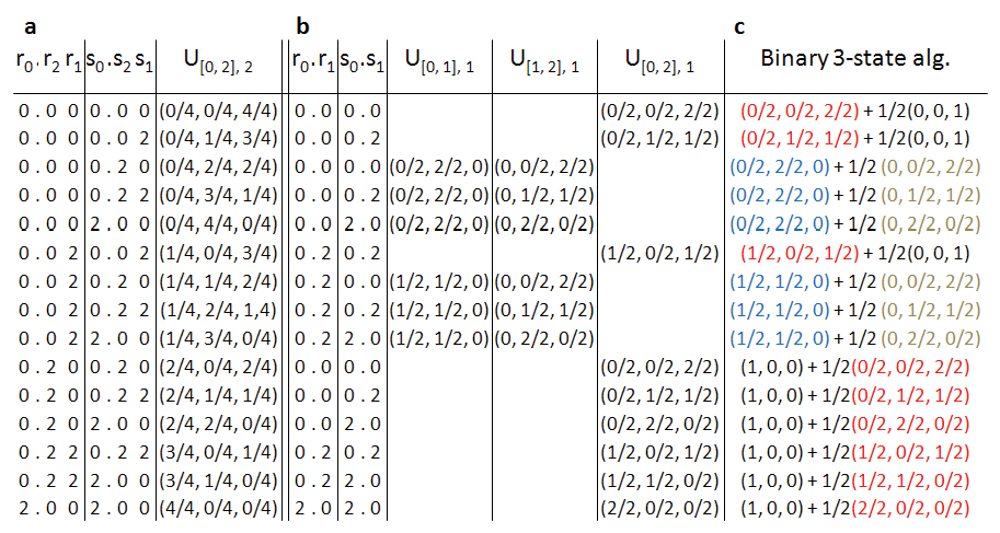
Refer to caption
Figure 13: 3-state UPG mapping The mapping for a UPG that generates distributions of the form (x04,x14,x24)subscript𝑥04subscript𝑥14subscript𝑥24(\frac{x_{0}}{4},\frac{x_{1}}{4},\frac{x_{2}}{4}). Here we notice that y0subscript𝑦0y_{0} is being used a couple of times. Again, we don’t make predictions about inputs that don’t correspond to a probability distribution: this includes both those with a sum greater than 1 and those for which the y𝑦y encoding is less than the x𝑥x encoding (which would mean a negative x12nsubscript𝑥1superscript2𝑛\frac{x_{1}}{2^{n}} value).
Theorem 8

A 2-state UPG Unsubscript𝑈𝑛U_{n} with inputs r0,rn,,r2,r1subscript𝑟0subscript𝑟𝑛subscript𝑟2subscript𝑟1r_{0},r_{n},\ldots,r_{2},r_{1} can be constructed with a linear number of switches using either of the two recursive constructions in Figure 14, where the n bits used in Un1subscript𝑈𝑛1U_{n-1} are r0,rn1,,r2,r1subscript𝑟0subscript𝑟𝑛1subscript𝑟2subscript𝑟1r_{0},r_{n-1},\ldots,r_{2},r_{1}.

Proof:

We prove that the circuits in Figure 12 and Figure 14 are equivalent by using induction. Base Case: U0=r¯0=r¯0U0subscript𝑈0subscript¯𝑟0subscript¯𝑟0subscriptsuperscript𝑈0U_{0}=\bar{r}_{0}=\bar{r}_{0}U^{\prime}_{0}

Inductive Step: Assume that Un1=r0Un1subscript𝑈𝑛1subscript𝑟0subscriptsuperscript𝑈𝑛1U_{n-1}=r_{0}U^{\prime}_{n-1}. Then,

Unsubscript𝑈𝑛\displaystyle U_{n} =Un1(r¯nr¯0+pn)+pnr¯nr¯0absentsubscript𝑈𝑛1subscript¯𝑟𝑛subscript¯𝑟0subscript𝑝𝑛subscript𝑝𝑛subscript¯𝑟𝑛subscript¯𝑟0\displaystyle=U_{n-1}(\bar{r}_{n}\bar{r}_{0}+p_{n})+p_{n}\bar{r}_{n}\bar{r}_{0}
=r¯0Un1(r¯nr¯0+pn)+pnr¯nr¯0absentsubscript¯𝑟0subscriptsuperscript𝑈𝑛1subscript¯𝑟𝑛subscript¯𝑟0subscript𝑝𝑛subscript𝑝𝑛subscript¯𝑟𝑛subscript¯𝑟0\displaystyle=\bar{r}_{0}U^{\prime}_{n-1}(\bar{r}_{n}\bar{r}_{0}+p_{n})+p_{n}\bar{r}_{n}\bar{r}_{0}
=r¯0(Un1(r¯nr¯0+pn)+pnr¯n)absentsubscript¯𝑟0subscriptsuperscript𝑈𝑛1subscript¯𝑟𝑛subscript¯𝑟0subscript𝑝𝑛subscript𝑝𝑛subscript¯𝑟𝑛\displaystyle=\bar{r}_{0}(U^{\prime}_{n-1}(\bar{r}_{n}\bar{r}_{0}+p_{n})+p_{n}\bar{r}_{n})
=r¯0(Un1(r¯n+pn)+pnr¯n)absentsubscript¯𝑟0subscriptsuperscript𝑈𝑛1subscript¯𝑟𝑛subscript𝑝𝑛subscript𝑝𝑛subscript¯𝑟𝑛\displaystyle=\bar{r}_{0}(U^{\prime}_{n-1}(\bar{r}_{n}+p_{n})+p_{n}\bar{r}_{n})
=r¯0Unabsentsubscript¯𝑟0subscriptsuperscript𝑈𝑛\displaystyle=\bar{r}_{0}U^{\prime}_{n}

In this final form, the series-parallel circuit uses 2n2𝑛2n pswitches and 2n+12𝑛12n+1 deterministic switches. The non-sp construction uses n𝑛n pswitches and 3n+13𝑛13n+1 deterministic switches.

Before we can generalize to N𝑁N states, we need to define some new notation and equalities. Define the 2-state UPG U[i,i+1],nsubscript𝑈𝑖𝑖1𝑛U_{[i,i+1],n} to be a circuit generating probability x02nsubscript𝑥0superscript2𝑛\frac{x_{0}}{2^{n}} on state i𝑖i and x12nsubscript𝑥1superscript2𝑛\frac{x_{1}}{2^{n}} on state i+1𝑖1i+1.

Under this notation, the previous results we proved were for U[0,1],nsubscript𝑈01𝑛U_{[0,1],n}. We can extend these results to U[i,i+1],nsubscript𝑈𝑖𝑖1𝑛U_{[i,i+1],n} with the following changes:

  1. 1.

    The input bits 𝐫𝐫\mathbf{r} will take on values i𝑖i and i+1𝑖1i+1 instead of 00 and 111 respectively

  2. 2.

    The pswitch pnsubscript𝑝𝑛p_{n} will take on values i𝑖i and i+1𝑖1i+1 with 1212\frac{1}{2} probability each instead of taking on values 00, 111 with equal probability.

But what if we didn’t use values i𝑖i and i+1𝑖1i+1 for 𝐫,pn𝐫subscript𝑝𝑛\mathbf{r},p_{n}?

Lemma 7

Let U[i,i+1],n(a,b)subscript𝑈𝑖𝑖1𝑛𝑎𝑏U_{[i,i+1],n}(a,b) be a circuit identical to U[i,i+1],nsubscript𝑈𝑖𝑖1𝑛U_{[i,i+1],n} except that 𝐫,pn𝐫subscript𝑝𝑛\mathbf{r},p_{n} take on values a𝑎a and b𝑏b. Our previous results for probability generation are for U[i,i+1],n(i,i+1)subscript𝑈𝑖𝑖1𝑛𝑖𝑖1U_{[i,i+1],n}(i,i+1). Then if ai𝑎𝑖a\leq i, bi+1𝑏𝑖1b\geq i+1,

U[i,i+1],n(i,i+1)=(i+U[i,i+1],n(a,b))(i+1)subscript𝑈𝑖𝑖1𝑛𝑖𝑖1𝑖subscript𝑈𝑖𝑖1𝑛𝑎𝑏𝑖1\displaystyle U_{[i,i+1],n}(i,i+1)=(i+U_{[i,i+1],n}(a,b))(i+1)
Proof:

U[i,i+1],n(a,b)subscript𝑈𝑖𝑖1𝑛𝑎𝑏U_{[i,i+1],n}(a,b) will realize the desired distribution on states a𝑎a and b𝑏b. Then if ai𝑎𝑖a\leq i, bi+1𝑏𝑖1b\geq i+1, it is trivially that taking the max of i𝑖i and the min of i+1𝑖1i+1 will give us the same distribution on states i𝑖i and i+1𝑖1i+1. ∎

We want to avoid this messy notation for future generalizations. All future instances of U[i,i+1],nsubscript𝑈𝑖𝑖1𝑛U_{[i,i+1],n} are actually representing (i+U[i,i+1],n)(i+1)𝑖subscript𝑈𝑖𝑖1𝑛𝑖1(i+U_{[i,i+1],n})(i+1). In other words, U[i,i+1],nsubscript𝑈𝑖𝑖1𝑛U_{[i,i+1],n} will always generate the ‘correct’ distribution on states i𝑖i and i+1𝑖1i+1 as long as 𝐫,pn𝐫subscript𝑝𝑛\mathbf{r},p_{n} take on values ai𝑎𝑖a\leq i and bi+1𝑏𝑖1b\geq i+1.

Refer to caption
Figure 14: 2-state UPG removed bit Even though r0subscript𝑟0r_{0} was important in controlling the cases of our algorithm, it turns out we can remove it from the recursive construction and just append it at the end. Note that Unsubscriptsuperscript𝑈𝑛U^{\prime}_{n} only uses bits rn,,r2,r1subscript𝑟𝑛subscript𝑟2subscript𝑟1r_{n},\ldots,r_{2},r_{1}

VII-B 3-state UPG

Now we will derive the 3-state UPG by generalizing the steps we used in the 2-state UPG derivation. We first construct an exponential 3-state UPG that follows closely from the algorithm for realizing 3-state distributions. Then, we will algebraically reduce it to a quadratic construction and remove unnecessarily repetitive bits.

Definition: (3-state UPG). A 3-state UPG U[0,2],nsubscript𝑈02𝑛U_{[0,2],n} is a circuit that generates distributions of the form (x02n,x12n,x22n)subscript𝑥0superscript2𝑛subscript𝑥1superscript2𝑛subscript𝑥2superscript2𝑛(\frac{x_{0}}{2^{n}},\frac{x_{1}}{2^{n}},\frac{x_{2}}{2^{n}}) using 2 sets of n+1𝑛1n+1 input bits 𝐫,𝐬𝐫𝐬\mathbf{r},\mathbf{s}. These input bits will take on values 00 or 222; when the bits 𝐫𝐫\mathbf{r}, in the order r0,rn,rn1,,r2,r1subscript𝑟0subscript𝑟𝑛subscript𝑟𝑛1subscript𝑟2subscript𝑟1r_{0},r_{n},r_{n-1},\ldots,r_{2},r_{1} are set to the binary representation of x02nsubscript𝑥0superscript2𝑛\frac{x_{0}}{2^{n}} and the bits 𝐬𝐬\mathbf{s}, in the order s0,sn,sn1,,s2,s1subscript𝑠0subscript𝑠𝑛subscript𝑠𝑛1subscript𝑠2subscript𝑠1s_{0},s_{n},s_{n-1},\ldots,s_{2},s_{1} are set to the binary representation of x02n+x12nsubscript𝑥0superscript2𝑛subscript𝑥1superscript2𝑛\frac{x_{0}}{2^{n}}+\frac{x_{1}}{2^{n}} (with the symbol 2 replacing the boolean 1), then the circuit U[0,2],nsubscript𝑈02𝑛U_{[0,2],n} will realize distribution (x02n,x12n,x22n)subscript𝑥0superscript2𝑛subscript𝑥1superscript2𝑛subscript𝑥2superscript2𝑛(\frac{x_{0}}{2^{n}},\frac{x_{1}}{2^{n}},\frac{x_{2}}{2^{n}}). In other words, to realize any desired binary probability (x02n,x12n,x22n)subscript𝑥0superscript2𝑛subscript𝑥1superscript2𝑛subscript𝑥2superscript2𝑛(\frac{x_{0}}{2^{n}},\frac{x_{1}}{2^{n}},\frac{x_{2}}{2^{n}}), we set the input bits 𝐫𝐫\mathbf{r} and 𝐬𝐬\mathbf{s} to p0subscript𝑝0p_{0} and p0+p1subscript𝑝0subscript𝑝1p_{0}+p_{1} respectively.

As an example, we look at the input-output mappings for the circuit U[0,2],2subscript𝑈022U_{[0,2],2}. If we input 𝐫=002,𝐬=020formulae-sequence𝐫002𝐬020\mathbf{r}=002,\mathbf{s}=020, the circuit will realize (14,14,12)141412(\frac{1}{4},\frac{1}{4},\frac{1}{2}) since 14=0.01214subscript0.012\frac{1}{4}=0.01_{2} and 14+14=12=0.102141412subscript0.102\frac{1}{4}+\frac{1}{4}=\frac{1}{2}=0.10_{2}. The input 𝐫=020,𝐬=022formulae-sequence𝐫020𝐬022\mathbf{r}=020,\mathbf{s}=022 will realize (12,14,14)121414(\frac{1}{2},\frac{1}{4},\frac{1}{4}) since 12=0.10212subscript0.102\frac{1}{2}=0.10_{2} and 12+14=34=0.112121434subscript0.112\frac{1}{2}+\frac{1}{4}=\frac{3}{4}=0.11_{2}. (see Figure 13a).

Again, the motivation for the exponential UPG comes from an interesting property in the truth table of U[0,2],2subscript𝑈022U_{[0,2],2}. We first eumerate all outputs given inputs corresponding to valid probability distributions. For each row (input), we ask: What are the outputs of U[0,1],1,U[1,2],1,U[0,2],1subscript𝑈011subscript𝑈121subscript𝑈021U_{[0,1],1},U_{[1,2],1},U_{[0,2],1} if we use the inputs r0,r1subscript𝑟0subscript𝑟1r_{0},r_{1} for U[0,1],1subscript𝑈011U_{[0,1],1}, the inputs s0,s1subscript𝑠0subscript𝑠1s_{0},s_{1} for U[1,2],1subscript𝑈121U_{[1,2],1}, and r0,r1,s0,s1subscript𝑟0subscript𝑟1subscript𝑠0subscript𝑠1r_{0},r_{1},s_{0},s_{1} for U[0,2],2subscript𝑈022U_{[0,2],2}? Is there a relationship to the construction of the U[0,2],1subscript𝑈021U_{[0,2],1} output probability.

The answer is yes. We find that they are the same probability distributions that are used in the binary algorithm for 3-states (Fig. 13bc). We can now derive the exponential recursive construction.
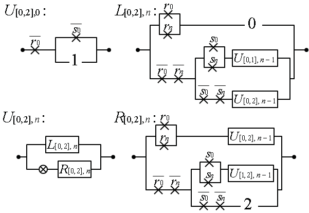
Refer to caption
Figure 15: 3-state exponential UPG We design a UPG directly from the algorithm. Note that this uses an exponential number of switches since the recursion uses two copies of U[0,2],n1subscript𝑈02𝑛1U_{[0,2],n-1}.
Lemma 8

A 3-state UPG U[0,2],nsubscript𝑈02𝑛U_{[0,2],n} with inputs r0,rn,,r2,r1subscript𝑟0subscript𝑟𝑛subscript𝑟2subscript𝑟1r_{0},r_{n},\ldots,r_{2},r_{1} and s0,sn,,s2,s1subscript𝑠0subscript𝑠𝑛subscript𝑠2subscript𝑠1s_{0},s_{n},\ldots,s_{2},s_{1} can be constructed with an exponential number of switches using the recursive construction in Figure 15, where the bits used in U[0,1],n1subscript𝑈01𝑛1U_{[0,1],n-1} are r0,rn1,,r2,r1subscript𝑟0subscript𝑟𝑛1subscript𝑟2subscript𝑟1r_{0},r_{n-1},\ldots,r_{2},r_{1}, the bits used in U[1,2],n1subscript𝑈12𝑛1U_{[1,2],n-1} are s0,sn1,,s2,s1subscript𝑠0subscript𝑠𝑛1subscript𝑠2subscript𝑠1s_{0},s_{n-1},\ldots,s_{2},s_{1}, and the bits used in U[0,2],n1subscript𝑈02𝑛1U_{[0,2],n-1} are r0,rn1,,r2,r1subscript𝑟0subscript𝑟𝑛1subscript𝑟2subscript𝑟1r_{0},r_{n-1},\ldots,r_{2},r_{1} and s0,sn1,,s2,s1subscript𝑠0subscript𝑠𝑛1subscript𝑠2subscript𝑠1s_{0},s_{n-1},\ldots,s_{2},s_{1}.

Proof:

We can prove this inductively.

Base Case: U[0,2],0=r¯0(s¯0+1)subscript𝑈020subscript¯𝑟0subscript¯𝑠01U_{[0,2],0}=\bar{r}_{0}(\bar{s}_{0}+1) realizes (1,0,0)100(1,0,0) when r0=2subscript𝑟02r_{0}=2, (0,1,0)010(0,1,0) when r0=0,s0=2formulae-sequencesubscript𝑟00subscript𝑠02r_{0}=0,s_{0}=2, and (0,0,1)001(0,0,1) when r0=0,s0=0formulae-sequencesubscript𝑟00subscript𝑠00r_{0}=0,s_{0}=0.

Inductive Step: Assume U[0,2],n1subscript𝑈02𝑛1U_{[0,2],n-1} realizes the correct distributions given the defined inputs. Then we want to show that

U[0,2],nsubscript𝑈02𝑛\displaystyle U_{[0,2],n} =L[0,2],n+(12,0,12)R[0,2],n,absentsubscript𝐿02𝑛12012subscript𝑅02𝑛\displaystyle=L_{[0,2],n}+(\frac{1}{2},0,\frac{1}{2})R_{[0,2],n},
L[0,2],nsubscript𝐿02𝑛\displaystyle L_{[0,2],n} =r0n0+r¯0n(s0nU[0,1],n1+s¯0nU[0,2],n1),absentsubscript𝑟0𝑛0subscript¯𝑟0𝑛subscript𝑠0𝑛subscript𝑈01𝑛1subscript¯𝑠0𝑛subscript𝑈02𝑛1\displaystyle=r_{0n}\cdot 0+\bar{r}_{0n}(s_{0n}U_{[0,1],n-1}+\bar{s}_{0n}U_{[0,2],n-1}),
R[0,2],nsubscript𝑅02𝑛\displaystyle R_{[0,2],n} =r0nU[0,2],n1+r¯0n(s0nU[1,2],n1+s¯0n2)absentsubscript𝑟0𝑛subscript𝑈02𝑛1subscript¯𝑟0𝑛subscript𝑠0𝑛subscript𝑈12𝑛1subscript¯𝑠0𝑛2\displaystyle=r_{0n}U_{[0,2],n-1}+\bar{r}_{0n}(s_{0n}U_{[1,2],n-1}+\bar{s}_{0n}\cdot 2)

This is equivalent to showing,

Ur,nsubscript𝑈𝑟𝑛\displaystyle U_{r,n} =Lr,n+(12,0,12)Rr,n,absentsubscript𝐿𝑟𝑛12012subscript𝑅𝑟𝑛\displaystyle=L_{r,n}+(\frac{1}{2},0,\frac{1}{2})R_{r,n},
Lr,nsubscript𝐿𝑟𝑛\displaystyle L_{r,n} ={(1,0,0), if r0n=2U[0,1],n1, if r¯0n=2,s0n=2U[0,2],n1, if r¯0n=2,s¯0n=2absentcases100 if subscript𝑟0𝑛2subscript𝑈01𝑛1formulae-sequence if subscript¯𝑟0𝑛2subscript𝑠0𝑛2subscript𝑈02𝑛1formulae-sequence if subscript¯𝑟0𝑛2subscript¯𝑠0𝑛2\displaystyle=\begin{cases}(1,0,0),&\text{ if }r_{0n}=2\\ U_{[0,1],n-1},&\text{ if }\bar{r}_{0n}=2,s_{0n}=2\\ U_{[0,2],n-1},&\text{ if }\bar{r}_{0n}=2,\bar{s}_{0n}=2\end{cases}
Rr,nsubscript𝑅𝑟𝑛\displaystyle R_{r,n} ={U[0,2],n1, if r0n=2U[1,2],n1, if r¯0n=2,s0n=2(0,0,1), if r¯0n=2,s¯0n=2absentcasessubscript𝑈02𝑛1 if subscript𝑟0𝑛2subscript𝑈12𝑛1formulae-sequence if subscript¯𝑟0𝑛2subscript𝑠0𝑛2001formulae-sequence if subscript¯𝑟0𝑛2subscript¯𝑠0𝑛2\displaystyle=\begin{cases}U_{[0,2],n-1},&\text{ if }r_{0n}=2\\ U_{[1,2],n-1},&\text{ if }\bar{r}_{0n}=2,s_{0n}=2\\ (0,0,1),&\text{ if }\bar{r}_{0n}=2,\bar{s}_{0n}=2\end{cases}

which is equivalent to showing,

U[0,2],nsubscript𝑈02𝑛\displaystyle U_{[0,2],n} ={(1,0,0)+(12,0,12)U[0,2],n1, if r0n=2U[0,1],n1+(12,0,12)U[1,2],n1, if r¯0n=2,s0n=2U[0,2],n1+(12,0,12)(0,0,1), if r¯0n=2,s¯0n=2absentcases10012012subscript𝑈02𝑛1 if subscript𝑟0𝑛2subscript𝑈01𝑛112012subscript𝑈12𝑛1formulae-sequence if subscript¯𝑟0𝑛2subscript𝑠0𝑛2subscript𝑈02𝑛112012001formulae-sequence if subscript¯𝑟0𝑛2subscript¯𝑠0𝑛2\displaystyle=\begin{cases}(1,0,0)+(\frac{1}{2},0,\frac{1}{2})U_{[0,2],n-1},&\text{ if }r_{0n}=2\\ U_{[0,1],n-1}+(\frac{1}{2},0,\frac{1}{2})U_{[1,2],n-1},&\text{ if }\bar{r}_{0n}=2,s_{0n}=2\\ U_{[0,2],n-1}+(\frac{1}{2},0,\frac{1}{2})(0,0,1),&\text{ if }\bar{r}_{0n}=2,\bar{s}_{0n}=2\end{cases}

Here, we are reminded of the algorithm for realizing any 3-state binary distribution: (x02n,x12n,x22n)=subscript𝑥0superscript2𝑛subscript𝑥1superscript2𝑛subscript𝑥2superscript2𝑛absent(\frac{x_{0}}{2^{n}},\frac{x_{1}}{2^{n}},\frac{x_{2}}{2^{n}})=

{(1,0,0)+12(x02n11,x12n1,x22n1), if x02n12(x02n1,x1+x22n11,0)+12(0,x0+x12n11,x22n1), if x02n<12,x0+x12n12(x02n1,x12n1,x22n11)+12(0,0,1), if x02n<12,x0+x12n<12cases10012subscript𝑥0superscript2𝑛11subscript𝑥1superscript2𝑛1subscript𝑥2superscript2𝑛1 if subscript𝑥0superscript2𝑛12subscript𝑥0superscript2𝑛1subscript𝑥1subscript𝑥2superscript2𝑛110120subscript𝑥0subscript𝑥1superscript2𝑛11subscript𝑥2superscript2𝑛1 if subscript𝑥0superscript2𝑛12otherwisesubscript𝑥0subscript𝑥1superscript2𝑛12subscript𝑥0superscript2𝑛1subscript𝑥1superscript2𝑛1subscript𝑥2superscript2𝑛1112001 if subscript𝑥0superscript2𝑛12otherwisesubscript𝑥0subscript𝑥1superscript2𝑛12\displaystyle\begin{cases}(1,0,0)+\frac{1}{2}(\frac{x_{0}}{2^{n-1}}-1,\frac{x_{1}}{2^{n-1}},\frac{x_{2}}{2^{n-1}}),&\text{ if }\frac{x_{0}}{2^{n}}\geq\frac{1}{2}\\ (\frac{x_{0}}{2^{n-1}},\frac{x_{1}+x_{2}}{2^{n-1}}-1,0)+\frac{1}{2}(0,\frac{x_{0}+x_{1}}{2^{n-1}}-1,\frac{x_{2}}{2^{n-1}}),&\text{ if }\frac{x_{0}}{2^{n}}<\frac{1}{2},\\ &\frac{x_{0}+x_{1}}{2^{n}}\geq\frac{1}{2}\\ (\frac{x_{0}}{2^{n-1}},\frac{x_{1}}{2^{n-1}},\frac{x_{2}}{2^{n-1}}-1)+\frac{1}{2}(0,0,1),&\text{ if }\frac{x_{0}}{2^{n}}<\frac{1}{2},\\ &\frac{x_{0}+x_{1}}{2^{n}}<\frac{1}{2}\end{cases}

From here, it is straightforward to complete our proof. r0n=2x02n12iffsubscript𝑟0𝑛2subscript𝑥0superscript2𝑛12r_{0n}=2\iff\frac{x_{0}}{2^{n}}\geq\frac{1}{2}, r¯0n=2x02n<12iffsubscript¯𝑟0𝑛2subscript𝑥0superscript2𝑛12\bar{r}_{0n}=2\iff\frac{x_{0}}{2^{n}}<\frac{1}{2}, s0n=2x0+x12n12iffsubscript𝑠0𝑛2subscript𝑥0subscript𝑥1superscript2𝑛12s_{0n}=2\iff\frac{x_{0}+x_{1}}{2^{n}}\geq\frac{1}{2}, and s¯0n=2x0+x12n<12iffsubscript¯𝑠0𝑛2subscript𝑥0subscript𝑥1superscript2𝑛12\bar{s}_{0n}=2\iff\frac{x_{0}+x_{1}}{2^{n}}<\frac{1}{2}. In addition, if 𝐫,𝐬𝐫𝐬\mathbf{r},\mathbf{s} are set to generate (x02n,x12n,x22n)subscript𝑥0superscript2𝑛subscript𝑥1superscript2𝑛subscript𝑥2superscript2𝑛(\frac{x_{0}}{2^{n}},\frac{x_{1}}{2^{n}},\frac{x_{2}}{2^{n}}), then using r0,rn1,,r2,r1subscript𝑟0subscript𝑟𝑛1subscript𝑟2subscript𝑟1r_{0},r_{n-1},\ldots,r_{2},r_{1} and s0,sn1,,s2,s1subscript𝑠0subscript𝑠𝑛1subscript𝑠2subscript𝑠1s_{0},s_{n-1},\ldots,s_{2},s_{1} as inputs to U[0,1],n1subscript𝑈01𝑛1U_{[0,1],n-1}, U[1,2],n1subscript𝑈12𝑛1U_{[1,2],n-1} and U[0,2],n1subscript𝑈02𝑛1U_{[0,2],n-1} we get the corresponding values to the 3-state binary algorithm. Then we can conclude that U[0,2],nsubscript𝑈02𝑛U_{[0,2],n} will successfully realize (x02n,x12n,x22n)subscript𝑥0superscript2𝑛subscript𝑥1superscript2𝑛subscript𝑥2superscript2𝑛(\frac{x_{0}}{2^{n}},\frac{x_{1}}{2^{n}},\frac{x_{2}}{2^{n}}). ∎

Refer to caption
Figure 16: 3-state UPG reduced After reducing the exponential UPG, we get two linear UPGs. One is a sp-circuit and uses 2 stochastic switches. The other is non-sp and uses 1 stochastic switch.
Lemma 9

A 3-state UPG U[0,2],nsubscript𝑈02𝑛U_{[0,2],n} with inputs r0,rn,,r2,r1subscript𝑟0subscript𝑟𝑛subscript𝑟2subscript𝑟1r_{0},r_{n},\ldots,r_{2},r_{1} and s0,sn,,s2,s1subscript𝑠0subscript𝑠𝑛subscript𝑠2subscript𝑠1s_{0},s_{n},\ldots,s_{2},s_{1} can be constructed with a quadratic number of switches using either of the two recursive constructions in Figure 16, where the bits used in U[0,1],n1subscript𝑈01𝑛1U_{[0,1],n-1} are r0,rn1,,r2,r1subscript𝑟0subscript𝑟𝑛1subscript𝑟2subscript𝑟1r_{0},r_{n-1},\ldots,r_{2},r_{1}, the bits used in U[1,2],n1subscript𝑈12𝑛1U_{[1,2],n-1} are s0,sn1,,s2,s1subscript𝑠0subscript𝑠𝑛1subscript𝑠2subscript𝑠1s_{0},s_{n-1},\ldots,s_{2},s_{1}, and the bits used in U[0,2],n1subscript𝑈02𝑛1U_{[0,2],n-1} are r0,rn1,,r2,r1subscript𝑟0subscript𝑟𝑛1subscript𝑟2subscript𝑟1r_{0},r_{n-1},\ldots,r_{2},r_{1} and s0,sn1,,s2,s1subscript𝑠0subscript𝑠𝑛1subscript𝑠2subscript𝑠1s_{0},s_{n-1},\ldots,s_{2},s_{1}.

Proof:

We will prove this by algebraically reducing the exponential UPG. Let pi=(12,0,12)subscript𝑝𝑖12012p_{i}=(\frac{1}{2},0,\frac{1}{2}) be i.i.d. We also introduce some new variables to make the final expressions concise.

L[0,2],n1superscriptsubscript𝐿02𝑛1\displaystyle L_{[0,2],n}^{1} =s0nU[0,1],n1+s¯0n2,absentsubscript𝑠0𝑛subscript𝑈01𝑛1subscript¯𝑠0𝑛2\displaystyle=s_{0n}U_{[0,1],n-1}+\bar{s}_{0n}\cdot 2,
R[0,2],n1superscriptsubscript𝑅02𝑛1\displaystyle R_{[0,2],n}^{1} =s0nU[1,2],n1+s¯0n2absentsubscript𝑠0𝑛subscript𝑈12𝑛1subscript¯𝑠0𝑛2\displaystyle=s_{0n}U_{[1,2],n-1}+\bar{s}_{0n}\cdot 2

A visual of these is in Figure 16. R[0,2],n1superscriptsubscript𝑅02𝑛1R_{[0,2],n}^{1} is defined so that R[0,2],n=r0nU[0,2],n1+r¯0nR[0,2],n1subscript𝑅02𝑛subscript𝑟0𝑛subscript𝑈02𝑛1subscript¯𝑟0𝑛superscriptsubscript𝑅02𝑛1R_{[0,2],n}=r_{0n}U_{[0,2],n-1}+\bar{r}_{0n}R_{[0,2],n}^{1}. L[0,2],n1superscriptsubscript𝐿02𝑛1L_{[0,2],n}^{1} is defined similarly except that the U[0,2],n1subscript𝑈02𝑛1U_{[0,2],n-1} component is replaced by a 222. We notice that,

L[0,2],nsubscript𝐿02𝑛\displaystyle L_{[0,2],n} =U[0,2],n1L[0,2],nabsentsubscript𝑈02𝑛1subscript𝐿02𝑛\displaystyle=U_{[0,2],n-1}L_{[0,2],n}
=U[0,2],n1(r0n0+r¯0nL[0,1],n11)absentsubscript𝑈02𝑛1subscript𝑟0𝑛0subscript¯𝑟0𝑛superscriptsubscript𝐿01𝑛11\displaystyle=U_{[0,2],n-1}(r_{0n}\cdot 0+\bar{r}_{0n}L_{[0,1],n-1}^{1})
U[0,2],nsubscript𝑈02𝑛\displaystyle U_{[0,2],n} =L[0,2],n+pnR[0,2],nabsentsubscript𝐿02𝑛subscript𝑝𝑛subscript𝑅02𝑛\displaystyle=L_{[0,2],n}+p_{n}R_{[0,2],n}
=L[0,2],nU[0,2],n1+pnR[0,2],nabsentsubscript𝐿02𝑛subscript𝑈02𝑛1subscript𝑝𝑛subscript𝑅02𝑛\displaystyle=L_{[0,2],n}U_{[0,2],n-1}+p_{n}R_{[0,2],n}
=(r0n0+r¯0nL[0,2],n1)U[0,2],n1absentsubscript𝑟0𝑛0subscript¯𝑟0𝑛superscriptsubscript𝐿02𝑛1subscript𝑈02𝑛1\displaystyle=(r_{0n}\cdot 0+\bar{r}_{0n}L_{[0,2],n}^{1})U_{[0,2],n-1}
+pn(r0nU[0,2],n1+r¯0nR[0,2],n1)subscript𝑝𝑛subscript𝑟0𝑛subscript𝑈02𝑛1subscript¯𝑟0𝑛superscriptsubscript𝑅02𝑛1\displaystyle\ \ \ \ +p_{n}(r_{0n}U_{[0,2],n-1}+\bar{r}_{0n}R_{[0,2],n}^{1})
=r¯0nL[0,2],n1U[0,2],n1+pn(r0nU[0,2],n1+r¯0nR[0,2],n1)absentsubscript¯𝑟0𝑛superscriptsubscript𝐿02𝑛1subscript𝑈02𝑛1subscript𝑝𝑛subscript𝑟0𝑛subscript𝑈02𝑛1subscript¯𝑟0𝑛superscriptsubscript𝑅02𝑛1\displaystyle=\bar{r}_{0n}L_{[0,2],n}^{1}U_{[0,2],n-1}+p_{n}(r_{0n}U_{[0,2],n-1}+\bar{r}_{0n}R_{[0,2],n}^{1})
=U[0,2],n1(r¯0nL[0,2],n1+pnr0n)+pnr¯0nR[0,2],n1absentsubscript𝑈02𝑛1subscript¯𝑟0𝑛superscriptsubscript𝐿02𝑛1subscript𝑝𝑛subscript𝑟0𝑛subscript𝑝𝑛subscript¯𝑟0𝑛superscriptsubscript𝑅02𝑛1\displaystyle=U_{[0,2],n-1}(\bar{r}_{0n}L_{[0,2],n}^{1}+p_{n}r_{0n})+p_{n}\bar{r}_{0n}R_{[0,2],n}^{1}

This is exactly the form of the series parallel construction in Figure 16.

U[0,2],nsubscript𝑈02𝑛\displaystyle U_{[0,2],n} =L[0,2],n+pnR[0,2],nabsentsubscript𝐿02𝑛subscript𝑝𝑛subscript𝑅02𝑛\displaystyle=L_{[0,2],n}+p_{n}R_{[0,2],n}
=L[0,2],nU[0,2],n1+pnR[0,2],nabsentsubscript𝐿02𝑛subscript𝑈02𝑛1subscript𝑝𝑛subscript𝑅02𝑛\displaystyle=L_{[0,2],n}U_{[0,2],n-1}+p_{n}R_{[0,2],n}
=(r0n0+r¯0nL[0,2],n1)U[0,2],n1absentsubscript𝑟0𝑛0subscript¯𝑟0𝑛superscriptsubscript𝐿02𝑛1subscript𝑈02𝑛1\displaystyle=(r_{0n}\cdot 0+\bar{r}_{0n}L_{[0,2],n}^{1})U_{[0,2],n-1}
+pn(r0nU[0,2],n1+r¯0nR[0,2],n1)subscript𝑝𝑛subscript𝑟0𝑛subscript𝑈02𝑛1subscript¯𝑟0𝑛superscriptsubscript𝑅02𝑛1\displaystyle\ \ \ \ +p_{n}(r_{0n}U_{[0,2],n-1}+\bar{r}_{0n}R_{[0,2],n}^{1})
=r¯0nL[0,2],n1U[0,2],n1+pn(r0nU[0,2],n1+r¯0nR[0,2],n1)absentsubscript¯𝑟0𝑛superscriptsubscript𝐿02𝑛1subscript𝑈02𝑛1subscript𝑝𝑛subscript𝑟0𝑛subscript𝑈02𝑛1subscript¯𝑟0𝑛superscriptsubscript𝑅02𝑛1\displaystyle=\bar{r}_{0n}L_{[0,2],n}^{1}U_{[0,2],n-1}+p_{n}(r_{0n}U_{[0,2],n-1}+\bar{r}_{0n}R_{[0,2],n}^{1})
=[U[0,2],n1][r¯0nL[0,2],n1]+[r¯0nR[0,2],n1][r0n][r¯0nL[0,2],n1]absentdelimited-[]subscript𝑈02𝑛1delimited-[]subscript¯𝑟0𝑛superscriptsubscript𝐿02𝑛1delimited-[]subscript¯𝑟0𝑛superscriptsubscript𝑅02𝑛1delimited-[]subscript𝑟0𝑛delimited-[]subscript¯𝑟0𝑛superscriptsubscript𝐿02𝑛1\displaystyle=[U_{[0,2],n-1}][\bar{r}_{0n}L_{[0,2],n}^{1}]+[\bar{r}_{0n}R_{[0,2],n}^{1}][r_{0n}][\bar{r}_{0n}L_{[0,2],n}^{1}]
+[U[0,2],n1][r0n][pn]+[r¯0nR[0,2],n1][pn]delimited-[]subscript𝑈02𝑛1delimited-[]subscript𝑟0𝑛delimited-[]subscript𝑝𝑛delimited-[]subscript¯𝑟0𝑛superscriptsubscript𝑅02𝑛1delimited-[]subscript𝑝𝑛\displaystyle\ \ \ \ +[U_{[0,2],n-1}][r_{0n}][p_{n}]+[\bar{r}_{0n}R_{[0,2],n}^{1}][p_{n}]

This is exactly the form of the non-series parallel construction in Figure 16. ∎

Finally, as in the 2-state UPG, we will remove the repetitive instances of r0subscript𝑟0r_{0} and s0subscript𝑠0s_{0}.

Refer to caption
Figure 17: 3-state UPG removed bit Even though r0subscript𝑟0r_{0} and s0subscript𝑠0s_{0} were important in controlling the cases of our algorithm, it turns out we can remove it from the recursive construction and just append it at the end.
Refer to caption
Figure 18: N𝑁N-state UPG The N𝑁N-state UPG is almost exactly the same as the 3-state UPG.
Theorem 9

A 3-state UPG U[0,2],nsubscript𝑈02𝑛U_{[0,2],n} with inputs r0,rn,,r2,r1subscript𝑟0subscript𝑟𝑛subscript𝑟2subscript𝑟1r_{0},r_{n},\ldots,r_{2},r_{1} and s0,sn,,s2,s1subscript𝑠0subscript𝑠𝑛subscript𝑠2subscript𝑠1s_{0},s_{n},\ldots,s_{2},s_{1} can be constructed with a quadratic number of switches using either of the two recursive constructions in Figure 17, where the bits used in U[0,1],n1subscript𝑈01𝑛1U_{[0,1],n-1} are r0,rn1,,r2,r1subscript𝑟0subscript𝑟𝑛1subscript𝑟2subscript𝑟1r_{0},r_{n-1},\ldots,r_{2},r_{1}, the bits used in U[1,2],n1subscript𝑈12𝑛1U_{[1,2],n-1} are s0,sn1,,s2,s1subscript𝑠0subscript𝑠𝑛1subscript𝑠2subscript𝑠1s_{0},s_{n-1},\ldots,s_{2},s_{1}, and the bits used in U[0,2],n1subscript𝑈02𝑛1U_{[0,2],n-1} are r0,rn1,,r2,r1subscript𝑟0subscript𝑟𝑛1subscript𝑟2subscript𝑟1r_{0},r_{n-1},\ldots,r_{2},r_{1} and s0,sn1,,s2,s1subscript𝑠0subscript𝑠𝑛1subscript𝑠2subscript𝑠1s_{0},s_{n-1},\ldots,s_{2},s_{1}.

Proof:

We will prove this by induction. Assume U[0,2],n1=r¯0(s¯0+1)U[0,2],n1subscript𝑈02𝑛1subscript¯𝑟0subscript¯𝑠01subscriptsuperscript𝑈02𝑛1U_{[0,2],n-1}=\bar{r}_{0}(\bar{s}_{0}+1)U^{\prime}_{[0,2],n-1}. Then, by breaking up the circuit into cases based on r0subscript𝑟0r_{0} and s0subscript𝑠0s_{0}, we will show that U[0,2],n=r¯0(s¯0+1)U[0,2],nsubscript𝑈02𝑛subscript¯𝑟0subscript¯𝑠01subscriptsuperscript𝑈02𝑛U_{[0,2],n}=\bar{r}_{0}(\bar{s}_{0}+1)U^{\prime}_{[0,2],n}.

Case 0: r0=2,s0=2formulae-sequencesubscript𝑟02subscript𝑠02r_{0}=2,s_{0}=2. In this case, we know that

U[0,2],nsubscript𝑈02𝑛\displaystyle U_{[0,2],n} =0absent0\displaystyle=0
r¯0subscript¯𝑟0\displaystyle\bar{r}_{0} =0r¯0(s¯0+1)U0,2],n=0\displaystyle=0\implies\bar{r}_{0}(\bar{s}_{0}+1)U^{\prime}_{0,2],n}=0

Therefore, U[0,2],n=r¯0(s¯0+1)U[0,2],nsubscript𝑈02𝑛subscript¯𝑟0subscript¯𝑠01subscriptsuperscript𝑈02𝑛U_{[0,2],n}=\bar{r}_{0}(\bar{s}_{0}+1)U^{\prime}_{[0,2],n}.

Case 1: r0=0,s0=2formulae-sequencesubscript𝑟00subscript𝑠02r_{0}=0,s_{0}=2.

U[0,2],nsubscript𝑈02𝑛\displaystyle U_{[0,2],n} =L[0,2],n+pnR[0,2],nabsentsubscript𝐿02𝑛subscript𝑝𝑛subscript𝑅02𝑛\displaystyle=L_{[0,2],n}+p_{n}R_{[0,2],n}
=L[0,2],nU[0,2],n1+pnR[0,2],nabsentsubscript𝐿02𝑛subscript𝑈02𝑛1subscript𝑝𝑛subscript𝑅02𝑛\displaystyle=L_{[0,2],n}U_{[0,2],n-1}+p_{n}R_{[0,2],n}
U[0,2],nsubscriptsuperscript𝑈02𝑛\displaystyle U^{\prime}_{[0,2],n} =L[0,2],n+pnR[0,2],nabsentsubscriptsuperscript𝐿02𝑛subscript𝑝𝑛subscriptsuperscript𝑅02𝑛\displaystyle=L^{\prime}_{[0,2],n}+p_{n}R^{\prime}_{[0,2],n}
=L[0,2],nU[0,2],n1+pnR[0,2],nabsentsubscriptsuperscript𝐿02𝑛subscriptsuperscript𝑈02𝑛1subscript𝑝𝑛subscriptsuperscript𝑅02𝑛\displaystyle=L^{\prime}_{[0,2],n}U^{\prime}_{[0,2],n-1}+p_{n}R^{\prime}_{[0,2],n}

We want to show that L[0,2],nU[0,2],n1=r¯0(s¯0+1)L[0,2],nU[0,2],n1subscript𝐿02𝑛subscript𝑈02𝑛1subscript¯𝑟0subscript¯𝑠01subscriptsuperscript𝐿02𝑛subscriptsuperscript𝑈02𝑛1L_{[0,2],n}U_{[0,2],n-1}=\bar{r}_{0}(\bar{s}_{0}+1)L^{\prime}_{[0,2],n}U^{\prime}_{[0,2],n-1}, R[0,2],n=r¯0(s¯0+1)R[0,2],nsubscript𝑅02𝑛subscript¯𝑟0subscript¯𝑠01subscriptsuperscript𝑅02𝑛R_{[0,2],n}=\bar{r}_{0}(\bar{s}_{0}+1)R^{\prime}_{[0,2],n}.

r¯0(s¯0+1)subscript¯𝑟0subscript¯𝑠01\displaystyle\bar{r}_{0}(\bar{s}_{0}+1) =1absent1\displaystyle=1
L[0,2],nU[0,2],n1subscriptsuperscript𝐿02𝑛subscriptsuperscript𝑈02𝑛1\displaystyle L^{\prime}_{[0,2],n}U^{\prime}_{[0,2],n-1} =r¯nU[0,1],n1absentsubscript¯𝑟𝑛subscriptsuperscript𝑈01𝑛1\displaystyle=\bar{r}_{n}U^{\prime}_{[0,1],n-1}
L[0,2],nU[0,2],n1subscript𝐿02𝑛subscript𝑈02𝑛1\displaystyle L_{[0,2],n}U_{[0,2],n-1} =r¯nU[0,1],n11U[0,2],n1absentsubscript¯𝑟𝑛subscript𝑈01𝑛11subscript𝑈02𝑛1\displaystyle=\bar{r}_{n}U_{[0,1],n-1}\cdot 1\cdot U_{[0,2],n-1}
=r¯nU[0,1],n11absentsubscript¯𝑟𝑛subscript𝑈01𝑛11\displaystyle=\bar{r}_{n}U_{[0,1],n-1}\cdot 1
=r¯n1U[0,1],n11absentsubscript¯𝑟𝑛1subscriptsuperscript𝑈01𝑛11\displaystyle=\bar{r}_{n}\cdot 1\cdot U^{\prime}_{[0,1],n-1}\cdot 1
=r¯0(s¯0+1)L[0,2],nU[0,2],n1absentsubscript¯𝑟0subscript¯𝑠01subscriptsuperscript𝐿02𝑛subscriptsuperscript𝑈02𝑛1\displaystyle=\bar{r}_{0}(\bar{s}_{0}+1)L^{\prime}_{[0,2],n}U^{\prime}_{[0,2],n-1}
R[0,2],nsubscriptsuperscript𝑅02𝑛\displaystyle R^{\prime}_{[0,2],n} =rnU[0,2],n1+r¯nabsentsubscript𝑟𝑛subscriptsuperscript𝑈02𝑛1subscript¯𝑟𝑛\displaystyle=r_{n}U^{\prime}_{[0,2],n-1}+\bar{r}_{n}
R[0,2],nsubscript𝑅02𝑛\displaystyle R_{[0,2],n} =rnU[0,2],n1+r¯n(U[1,2],n1+1)absentsubscript𝑟𝑛subscript𝑈02𝑛1subscript¯𝑟𝑛subscript𝑈12𝑛11\displaystyle=r_{n}U_{[0,2],n-1}+\bar{r}_{n}(U_{[1,2],n-1}+1)
=rnU[0,2],n11+r¯n1absentsubscript𝑟𝑛subscript𝑈02𝑛11subscript¯𝑟𝑛1\displaystyle=r_{n}U_{[0,2],n-1}\cdot 1+\bar{r}_{n}\cdot 1
=rn1U[0,2],n11+r¯n1absentsubscript𝑟𝑛1subscriptsuperscript𝑈02𝑛11subscript¯𝑟𝑛1\displaystyle=r_{n}\cdot 1\cdot U^{\prime}_{[0,2],n-1}\cdot 1+\bar{r}_{n}\cdot 1
=r¯0(s¯0+1)R[0,2],nabsentsubscript¯𝑟0subscript¯𝑠01subscriptsuperscript𝑅02𝑛\displaystyle=\bar{r}_{0}(\bar{s}_{0}+1)R^{\prime}_{[0,2],n}

Therefore, U[0,2],n=r¯0(s¯0+1)U[0,2],nsubscript𝑈02𝑛subscript¯𝑟0subscript¯𝑠01subscriptsuperscript𝑈02𝑛U_{[0,2],n}=\bar{r}_{0}(\bar{s}_{0}+1)U^{\prime}_{[0,2],n}.

Case 2: r0=0,s0=0formulae-sequencesubscript𝑟00subscript𝑠00r_{0}=0,s_{0}=0. In this case, we know that

r0nsubscript𝑟0𝑛\displaystyle r_{0n} =rnabsentsubscript𝑟𝑛\displaystyle=r_{n}
s0nsubscript𝑠0𝑛\displaystyle s_{0n} =rnabsentsubscript𝑟𝑛\displaystyle=r_{n}
r¯0(s¯0+1)subscript¯𝑟0subscript¯𝑠01\displaystyle\bar{r}_{0}(\bar{s}_{0}+1) =2absent2\displaystyle=2

Therefore, r¯0(s¯0+1)U[0,2],n=U[0,2],n=U[0,2],nsubscript¯𝑟0subscript¯𝑠01subscriptsuperscript𝑈02𝑛subscriptsuperscript𝑈02𝑛subscript𝑈02𝑛\bar{r}_{0}(\bar{s}_{0}+1)U^{\prime}_{[0,2],n}=U^{\prime}_{[0,2],n}=U_{[0,2],n}. ∎

Finally, as in the 2-state case, the 3-state UPG U[i,i+2],nsubscript𝑈𝑖𝑖2𝑛U_{[i,i+2],n} will generate the appropriate distributions over the states i,i+1,i+2𝑖𝑖1𝑖2i,i+1,i+2.

VII-C N𝑁N-state UPG

The results will now be generalized to N𝑁N-states. The steps and the proof are all identical to the 3-state version except that the variables L𝐿L and R𝑅R are defined to be generalized constructions. Since they are identical, we will define the N𝑁N-state UPG and then jump to the conclusion and circuit diagrams.

Definition (N𝑁N-state UPG): A N𝑁N-state UPG U[0,N1],nsubscript𝑈0𝑁1𝑛U_{[0,N-1],n} is a circuit that generates distributions of the form (x02n,x12n,,xN12n)subscript𝑥0superscript2𝑛subscript𝑥1superscript2𝑛subscript𝑥𝑁1superscript2𝑛(\frac{x_{0}}{2^{n}},\frac{x_{1}}{2^{n}},...,\frac{x_{N-1}}{2^{n}}) using N1𝑁1N-1 input vectors 𝐫𝟎,𝐫𝟏subscript𝐫0subscript𝐫1\mathbf{r_{0}},\mathbf{r_{1}}, …, 𝐫𝐍𝟐subscript𝐫𝐍2\mathbf{r_{N-2}}, where each vector 𝐫𝐢subscript𝐫𝐢\mathbf{r_{i}} has n+1𝑛1n+1 bits ri0subscript𝑟𝑖0r_{i0}, ri1subscript𝑟𝑖1r_{i1}, …, rinsubscript𝑟𝑖𝑛r_{in}. When the input vectors 𝐫𝐢=(ri0,rin,ri(n1),,ri2,ri1)subscript𝐫𝐢subscript𝑟𝑖0subscript𝑟𝑖𝑛subscript𝑟𝑖𝑛1subscript𝑟𝑖2subscript𝑟𝑖1\mathbf{r_{i}}=(r_{i0},r_{in},r_{i(n-1)},\ldots,r_{i2},r_{i1}) are set to the binary representation of x0+x1++xi2nsubscript𝑥0subscript𝑥1subscript𝑥𝑖superscript2𝑛\frac{x_{0}+x_{1}+...+x_{i}}{2^{n}} with the symbol N1𝑁1N-1 replacing the boolean 1, then the circuit U[0,N1],nsubscript𝑈0𝑁1𝑛U_{[0,N-1],n} will realize distribution (x02n,x12n,,xN12n)subscript𝑥0superscript2𝑛subscript𝑥1superscript2𝑛subscript𝑥𝑁1superscript2𝑛(\frac{x_{0}}{2^{n}},\frac{x_{1}}{2^{n}},...,\frac{x_{N-1}}{2^{n}}). In other words, to generate any desired binary distribution (x02n,x12n,,xN12n)subscript𝑥0superscript2𝑛subscript𝑥1superscript2𝑛subscript𝑥𝑁1superscript2𝑛(\frac{x_{0}}{2^{n}},\frac{x_{1}}{2^{n}},...,\frac{x_{N-1}}{2^{n}}), we set the input vector 𝐫𝟎subscript𝐫0\mathbf{r_{0}} to x02nsubscript𝑥0superscript2𝑛\frac{x_{0}}{2^{n}}, the input vector 𝐫𝟏subscript𝐫1\mathbf{r_{1}} to the sum x0+x12n,subscript𝑥0subscript𝑥1superscript2𝑛\frac{x_{0}+x_{1}}{2^{n}},\ldots, and the input vector 𝐫𝐍𝟐subscript𝐫𝐍2\mathbf{r_{N-2}} to the sum x0+x1++xN22nsubscript𝑥0subscript𝑥1subscript𝑥𝑁2superscript2𝑛\frac{x_{0}+x_{1}+...+x_{N-2}}{2^{n}}.

Theorem 10

A N𝑁N-state UPG U[0,N1],nsubscript𝑈0𝑁1𝑛U_{[0,N-1],n} with inputs 𝐫𝐢,0iN2subscript𝐫𝐢0𝑖𝑁2\mathbf{r_{i}},0\leq i\leq N-2 can be constructed with a polynomial number of switches O(nN1)𝑂superscript𝑛𝑁1O(n^{N-1}) using either of the two recursive constructions in Figure 18, where the bits used in U[0,i],n1subscript𝑈0𝑖𝑛1U_{[0,i],n-1} are 𝐫𝟎,𝐫𝟏,,𝐫𝐢𝟏subscript𝐫0subscript𝐫1subscript𝐫𝐢1\mathbf{r_{0}},\mathbf{r_{1}},\ldots,\mathbf{r_{i-1}} and the bits used in U[i,N1],n1subscript𝑈𝑖𝑁1𝑛1U_{[i,N-1],n-1} are 𝐫𝐢,𝐫𝐢+𝟏,,𝐫𝐍𝟐subscript𝐫𝐢subscript𝐫𝐢1subscript𝐫𝐍2\mathbf{r_{i}},\mathbf{r_{i+1}},\ldots,\mathbf{r_{N-2}}.

VIII Partial Orders

All current work has been done on states that are a total order. i.e. 0<1<<n101𝑛10<1<...<n-1. It is interesting to think about a logic on states that are in a partial order. We perform a cursory examination of constructing probabilities on lattices that are partial orders and find that we cannot generate many distributions on partial orders.

Composition rules must be generalized again since you cannot take a max or min of incomparable states. Instead of max and min, we use the \vee (join) and \wedge (meet) operators respectively.

Theorem 11 (Partial Order Inexpressibility)

For the lattice in Figure 19b, no distributions of the form v=(0,1p,p,0)𝑣01𝑝𝑝0v=(0,1-p,p,0), where p0𝑝0p\geq 0 are realizable by building a sp circuit with any switch set unless (0,1p,p,0)01𝑝𝑝0(0,1-p,p,0) itself is in the switch set.

Proof:

Assume that v𝑣v is realizable by a series composition. That is, v=xy𝑣𝑥𝑦v=xy. Then,

v00subscript𝑣00\displaystyle\displaystyle v_{00} =x00+y00x00y00+x01y10+x10y01absentsubscript𝑥00subscript𝑦00subscript𝑥00subscript𝑦00subscript𝑥01subscript𝑦10subscript𝑥10subscript𝑦01\displaystyle=x_{00}+y_{00}-x_{00}y_{00}+x_{01}y_{10}+x_{10}y_{01}
x00=0 and y00=0absentsubscript𝑥000 and subscript𝑦000\displaystyle\Rightarrow x_{00}=0\text{ and }y_{00}=0
v11subscript𝑣11\displaystyle v_{11} =0absent0\displaystyle=0
x11=0 or x11=0absentsubscript𝑥110 or subscript𝑥110\displaystyle\Rightarrow x_{11}=0\text{ or }x_{11}=0

WLOG, we let x11=0subscript𝑥110x_{11}=0, so that,

v10subscript𝑣10\displaystyle\displaystyle v_{10} =x10y11+x11y10+x10y10absentsubscript𝑥10subscript𝑦11subscript𝑥11subscript𝑦10subscript𝑥10subscript𝑦10\displaystyle=x_{10}y_{11}+x_{11}y_{10}+x_{10}y_{10}
=x10y11+x10y10absentsubscript𝑥10subscript𝑦11subscript𝑥10subscript𝑦10\displaystyle=x_{10}y_{11}+x_{10}y_{10}
=x10(y11+y10)=pabsentsubscript𝑥10subscript𝑦11subscript𝑦10𝑝\displaystyle=x_{10}(y_{11}+y_{10})=p
x100absentsubscript𝑥100\displaystyle\Rightarrow x_{10}\neq 0
v01subscript𝑣01\displaystyle v_{01} =x01y11+x11y01+x01y01absentsubscript𝑥01subscript𝑦11subscript𝑥11subscript𝑦01subscript𝑥01subscript𝑦01\displaystyle=x_{01}y_{11}+x_{11}y_{01}+x_{01}y_{01}
=x01y11+x01y01absentsubscript𝑥01subscript𝑦11subscript𝑥01subscript𝑦01\displaystyle=x_{01}y_{11}+x_{01}y_{01}
=x01(y11+y01)=1pabsentsubscript𝑥01subscript𝑦11subscript𝑦011𝑝\displaystyle=x_{01}(y_{11}+y_{01})=1-p
x010absentsubscript𝑥010\displaystyle\Rightarrow x_{01}\neq 0
v00subscript𝑣00\displaystyle v_{00} =x01y10+x10y01absentsubscript𝑥01subscript𝑦10subscript𝑥10subscript𝑦01\displaystyle=x_{01}y_{10}+x_{10}y_{01}
y10=0 and y01=0absentsubscript𝑦100 and subscript𝑦010\displaystyle\Rightarrow y_{10}=0\text{ and }y_{01}=0
y11=1absentsubscript𝑦111\displaystyle\Rightarrow y_{11}=1
x=vabsent𝑥𝑣\displaystyle\Rightarrow x=v

But then we have x𝑥x = v𝑣v, so we have shown that need without v𝑣v itself, we cannot realize v𝑣v through a series connection. In the same way, we can show the same result for a parallel composition (left out since it is almost identical), which means that v𝑣v is not realizable with a sp circuit. ∎
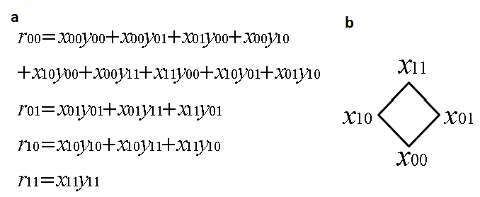
Refer to caption
Figure 19: A simple partially ordered lattice. This is an example of a simple partial order. (a) An example of a series composition (meet) of switches x𝑥x and y𝑦y. (b) The lattice structure.

IX Applications

One intuitive understanding of this multivalued alphabet is to think of timings and dependencies. Switches represent events, and the states represent the discrete time when the event occurs. When two switches x𝑥x and y𝑦y are composed to make the circuit z𝑧z, we are saying that for event z𝑧z to occur, it depends on events x𝑥x and y𝑦y. If event z𝑧z requires both x𝑥x and y𝑦y to occur before it can occur, then this can be represented by a parallel connection since the time z𝑧z occurs will be the max(x,y)𝑥𝑦\max(x,y). If event z𝑧z only needs either x𝑥x or y𝑦y to occur, then this can be represented by a series connection since the time z𝑧z occurs will be the min(x,y)𝑥𝑦\min(x,y).

It is possible to implement multivalued relay circuits using physical (open and closed) relay switches. If we consider switches as normally closed and the state as the time it is opened, then we have a direct correspondence to the description above. When switches are composed in series, the time that the entire circuit is open, is when either of the switches open (min) and when the switches are composed in parallel, the time that the entire circuit is open is when both the switches are open (max).

We can imagine a biological neural circuit working in a very similar way. Consider a network of neurons where each neuron only has incoming signals from 2 other neurons. Then, consider a neuron x𝑥x when incoming neurons y𝑦y and z𝑧z. Neuron x𝑥x will fires when the incoming signals exceeds a certain threshold potential. If the threshold is low, we can imagine that neuron x𝑥x will fire once it receives the first incoming signal (i.e. min(x,y)𝑥𝑦\min(x,y)). If the threshold is high, we can imagine that neuron x𝑥x will only fire if it receives signals from both incoming neurons (i.e. max(x,y)𝑥𝑦\max(x,y)). In general, with m𝑚m incoming neuron signals, it becomes slightly more complex; depending on the threshold of the neuron of interest, the time it fires would be when it receives the 1st, 2nd, 3rd, …, mth signal. These gates can be implemented by max/min gates.

There are a number of directions for extending this work to better model and understand biological circuits. These include studying joint distributions, stochastic functions, probability distributions on different state structures, and stochasticity in compositions. With further understanding of biological circuits, this can also aid in building artificial molecular circuits, such as in DNA computing[17]. In addition, stochastic circuits may be useful in modeling other stochastic networks in engineering.

X Conclusion

In this paper, we studied probability generation in the context of multivalued relay circuits, a generalization of two-state relays. We proved a duality result on this max/min generalization and then proved construction algorithms for generating any rational probability distribution. We extended the robustness result to these algorithms and showed that switch error remains bounded linearly regardless of the circuit size. Finally, we constructed a universal probability generator for mapping deterministic inputs to probability distributions and demonstrated a basic non-realizability result for partial orders.

Further work on multivalued stochastic switches may have many biological applications such as for neural coding.

Acknowledgment

The authors would like to thank Dan Wilhelm, Hongchao Zhou, and Ho-lin Chen for helpful discussions. They would also like to thank the Caltech SURF program, the Molecular Programming Project funded by the NSF Expeditions in Computing Program under grant CCF-0832824, and Aerospace Corporation for funding to make this research possible.

References

  • [1] J. von Neumann. Various techniques used in connection with random digits. Applied Math Series 12:36-38 (1951).
  • [2] D. Knuth, A. Yao. The complexity of nonuniform random number generation. Algorithms and Complexity: New Directions and Recent Results 357-428 (1976).
  • [3] T. Han, M. Hoshi. Interval algorithm for random number generation. IEEE Trans. on Information Theory 43(2):599-611 (1997).
  • [4] M. Elowitz, A. Levine, E. Siggia, P. Swain. Stochastic gene expression in a single cell. Science 297:183- 186 (2002).
  • [5] D. Soloveichik, M. Cook, E. Winfree, J. Bruck. Computation with finite stochastic chemical reaction networks. Natural Computing 7(4):615–633 (2008).
  • [6] E. Schneidman, B. Freedman, I. Segev. Ion channel stochasticity may be critical in determining the reliability and precision of spike timing. Neural Comp. 10:1679- 1703 (1998).
  • [7] J. Bruck. The logic of biological networks. Purdue University (2006). http://video.google.com/videoplay?docid=3684954164278324696.
  • [8] C. Shannon. A symbolic analysis of relay and switching circuits. Trans. AIEE 57:713–723 (1938).
  • [9] D. Wilhelm, J. Bruck. Stochastic switching circuit synthesis. Proc. IEEE ISIT (2008).
  • [10] H. Zhou, J. Bruck. On the expressibility of stochastic switching circuits. Proc. IEEE ISIT (2009).
  • [11] P. Loh, H. Zhou, J. Bruck. The robustness of stochastic switching networks. Proc. IEEE ISIT (2009).
  • [12] E. Post. Introduction to a general theory of elementary propositions. American Journal of Mathematics 43(3):163–185 (1921).
  • [13] D. Webb. Many-valued logics. Caltech Ph.D. Dissertation, Advisor Eric Bell (1936).
  • [14] D. Rine. Computer science and multiple-valued logic: theory and applications. North Holland (1984).
  • [15] J. Gunawardena. Min-max functions. Discrete Event Dynamic Systems: Theory and Applications 4(4):377 407 (1994).
  • [16] G. Shahaf, D. Eytan, A. Gal, E. Kermany, V. Lyakhov, et al. Order-based representation in random networks of cortical neurons. PLoS Comput. Biol. 4(11):e1000228 (2008).
  • [17] G. Seelig, D. Soloveichik, D. Zhang, E. Winfree. Enzyme-free nucleic acid logic circuits. Science 314:1585–1588 (2002).