Using Kuiper Belt Binaries to Constrain Neptune’s Migration History

Abstract

Approximately 10–20% of all Kuiper belt objects (KBOs) occupy mean-motion resonances with Neptune. This dynamical configuration likely resulted from resonance capture as Neptune migrated outward during the late stages of planet formation. The details of Neptune’s planetesimal-driven migration, including its radial extent and the concurrent eccentricity evolution of the planet, are the subject of considerable debate. Two qualitatively different proposals for resonance capture have been proposed—migration-induced capture driven by smooth outward evolution of Neptune’s orbit and chaotic capture driven by damping of the planet’s eccentricity near its current semi-major axis. We demonstrate that the distribution of comparable-mass, wide-separation binaries occupying resonant orbits can differentiate between these two scenarios. If migration-induced capture occurred, this fraction records information about the formation locations of different populations of KBOs. Chaotic capture, in contrast, randomizes the orbits of bodies as they are placed in resonance. In particular, if KBO binaries formed by dynamical capture in a protoplanetary disk with a surface mass density typical of observed extrasolar disks, then migration-induced capture produces the following signatures. The 2:1 resonance should contain a dynamically cold component, with inclinations less than 5–10^∘, having a binary fraction comparable to that among cold classical KBOs. If the 3:2 resonance also hosts a cold component, its binary fraction should be 20–30% lower than in the cold classical belt. Among cold 2:1 (and if present 3:2) KBOs, objects with eccentricities $e<0.2$ should have a binary fraction $\sim$20% larger than those with $e>0.2$. Other binary formation scenarios and disk surface density profiles can generate analogous signatures but produce quantitatively different results. Searches for cold components in the binary fractions of resonant KBOs are currently practical. The additional migration-generated trends described here may be distinguished with objects discovered by LSST.

1. INTRODUCTION

Our Kuiper belt, a $\sim$0.01–0.1$M_{\oplus}$ (e.g., Bernstein et al., 2004; Chiang et al., 2007; Fuentes & Holman, 2008) collection of planetesimal debris located beyond the orbit of Neptune, provides a unique window into the dynamical processes that shaped the young solar system. The orbits of Kuiper belt objects (KBOs) comprise a dynamical fossil, recording the movements of the giant planets during the era of their formation.

Though almost two decades have passed since the discovery of the first KBO after Pluto and Charon (Jewitt & Luu, 1993), and though the orbits of more than 500 trans-Neptunian objects have been well-characterized (e.g., Elliot et al., 2005; Kavelaars et al., 2009), a detailed theoretical understanding of the Kuiper belt’s rich dynamical structure remains elusive. For our purposes, we will focus on the following aspects of this structure, which remain difficult to reconcile.

• Approximately 10–20% of all KBOs, including Pluto and Charon, occupy mean motion resonances with Neptune (Jewitt et al., 1998; Trujillo et al., 2001; Kavelaars et al., 2009), and this fraction may be larger if many objects reside in distant resonances which are not yet well-characterized. In resonance, the orbital period of a KBO forms an approximate integer ratio with that of Neptune, leading to a coherent exchange of energy and angular momentum with the planet which is periodic over $\sim$$10^{4}$–$10^{5}$ year timescales. Though resonance occupation enhances long-term stability (e.g., Lykawka & Mukai, 2005), the large number of resonant KBOs suggests a special dynamical origin for this population.

• Several lines of evidence suggest that classical KBOs, those objects that are not in resonance and are not currently undergoing close encounters with Neptune (e.g., Gladman et al., 2008), consist of two populations with different histories and having different typical inclinations. The inclination distribution of the belt is bimodal, best fit by a population of bodies with $i\lesssim 5^{\circ}$ and a distinct population containing equal to greater mass with inclinations ranging up to $\sim$$35^{\circ}$ (Brown, 2001; Elliot et al., 2005; Gulbis et al., 2010). In addition, low and high inclination classical KBOs have systematically different physical properties. The high inclination population is bluer in color (Tegler & Romanishin, 2000; Trujillo & Brown, 2002; Peixinho et al., 2008), has a lower fraction of wide binaries (Stephens & Noll, 2006; Noll et al., 2008b), and contains all of the brightest (and hence likely largest) KBOs (Levison & Stern, 2001). The critical inclination separating those objects with bluer and redder colors is $\sim$$10^{\circ}$ rather than $\sim$$5^{\circ}$ (Lykawka & Mukai, 2005; Peixinho et al., 2008). The significance of this discrepancy, if any, is not yet known and may be complicated by overlap of the low and high inclination populations. Throughout this paper, we refer to this entire population as the classical belt, the low inclination subset as the cold classicals and the high inclination subset as the hot classicals. When specific numbers are used, we define “low inclination” as those objects with $i<10^{\circ}$ and “high inclination” as those with $i\geq 10^{\circ}$. We choose $10^{\circ}$ as our cutoff based on the distributions of colors with inclination because we will be investigating a physical property of KBOs—their binary fraction. Our conclusions will not change substantially if $5^{\circ}$ is determined to be more appropriate for the classical belt.

• Classical KBOs exist with eccentricities ranging up to $\sim$0.2. However, cold classical KBOs have systematically low eccentricities, likely reflecting a dynamically unexcited population. We note that for the purposes of this paper, “cold” and “hot” refer only to inclination.

• The inclinations of KBOs in 3:2 mean motion resonance span the same range as the inclinations of the classical belt, but the dynamical data may be fit with a single high inclination population (Gulbis et al., 2010).

• At $\sim$48 AU, the density of cold classical KBOs declines precipitously (Trujillo & Brown, 2001; Allen et al., 2002). This transition is located near Neptune’s 2:1 mean-motion resonance. Though the presence of the edge is clear, whether it is an edge in semi-major axis corresponding to the 2:1 resonance is less certain due to observational selection effects at these large distances from the Sun. Further, this edge may not be present in the hot classical population (Petit et al., in prep).

No dynamical model has yet simultaneously reproduced the inclination distribution of the belt, its eccentricity distribution, and the resonant population of KBOs.

Two qualitatively different explanations have been proposed for the abundance of KBOs occupying mean-motion resonances with Neptune. The first, which we refer to as “migration-induced capture,” was proposed by Malhotra (1993, 1995) to explain the orbit of Pluto. In this model, KBOs are captured into resonance as Neptune migrates outward during the late stages of planet formation. This migration is powered by planetesimal scattering in a disk containing $\sim$$30M_{\oplus}$ in planetesimals (Fernandez & Ip, 1984; Gomes et al., 2004), which also acts to damp the eccentricity and inclination of Neptune. In the simplest version of this scenario, Neptune migrates $\sim$10 AU with low eccentricity and inclination, though it may well have occupied a more excited orbit at earlier times. As this migration progresses, Neptune entrains KBOs in its mean motion resonances as the semi-major axes of the resonances sweep through the primordial planetesimal disk (Malhotra, 1993, 1995). This primordial disk must contain some KBOs with pre-excited eccentricities (Chiang et al., 2003) to explain the occupation of high-order resonances such as the 5:2. In this context, Levison & Morbidelli (2003) argue that the entire Kuiper belt might have been pushed out from closer to the Sun by migration, citing the belt’s low mass and external edge near Neptune’s 2:1 resonance.

As explored by Hahn & Malhotra (2005), early outward migration of Neptune reproduces the resonant structure of the belt well, but suffers from two difficulties. First, resonance capture excites the eccentricities of captured particles, but does not change their inclinations substantially, so inclinations must be excited prior to migration or an alternative inclination excitation mechanism must be found. Gomes (2003) argue that the large inclination objects in the belt may have arisen from scattered objects which interacted with secular resonances during migration. This process has a low efficiency (Chiang et al., 2007), however, making it difficult to explain the number of large inclination objects. Second, smooth migration does not sufficiently excite the eccentricities of non-resonant objects to explain the hot classical population of KBOs. Levison & Morbidelli (2003) argue that stochastic effects during migration could cause KBOs with excited eccentricities to be lost from resonance, populating the hot classical belt. However, Murray-Clay & Chiang (2006) demonstrate that for a substantial number of KBOs to be lost from resonance during migration, more than a few percent of the mass in the planetesimal disk driving migration must be in bodies with radii larger than $\mathcal{O}(1000{\rm km})$, comparable to the size of Pluto. This mass fraction is inconsistent with estimates of the size distribution in the early disk resulting from coagulation (e.g., Kenyon & Luu, 1999; Schlichting & Sari, 2011). Whether this conclusion is altered by recent models of planetesimal formation that may allow rapid formation of 100–1000 km bodies (Youdin & Goodman, 2005; Johansen et al., 2007) remains to be seen.

A third difficulty for migration-induced capture arises from the different inclination distributions in the classical Kuiper belt and the 3:2 resonant population. Resonant capture does not substantially alter inclinations, implying that the inclination distribution of a resonant population should match that of the population from which it captured its members. Though the 3:2 resonance did not pass through the region of the currently observed classical belt, it captured its population from an adjacent region of the protoplanetary disk, where one would naively expect the inclination distribution to be the same. Nevertheless, it is possible that objects caught into the 3:2 resonance experienced additional dynamical sculpting, rendering this expectation invalid, though no model for such sculpting as been produced thus far. In particular, we note that if distinct “hot” and “cold” populations exist in the 3:2 resonance, the characteristic inclination dividing these populations may not match that in the classical belt. The possibility of additional sculpting is less plausible for the 2:1 resonance, which did pass through the classical belt. Unfortunately, the inclination distribution of the 2:1 is not yet constrained well enough to confirm or rule out a cold component.

A second possibility for the population of mean-motion resonances was suggested more recently, inspired by the Nice model for the early evolution of the solar system giants (Tsiganis et al., 2005). In this model, Jupiter and Saturn cross their mutual 2:1 mean motion resonance as a result of migration driven by planetesimal scattering. This resonance passage substantially alters the orbits of Uranus and Neptune. Levison et al. (2008) argue that it is difficult to place Neptune interior to 21 AU at the end of the Nice model, and suggest chaotic population of the Kuiper belt as an alternative to migration-induced resonance capture. They argue that Neptune was scattered, with large eccentricity, onto an orbit with a semi-major axis close to its current value of 30 AU. Conservation of angular momentum during the scattering event leaves the planet on a low-inclination orbit. Initially after the scattering, orbits with semi-major axes ranging from that of Neptune out to its 2:1 resonance are chaotic. This chaos results from overlapping mean-motion resonances which are rendered wide by Neptune’s large eccentricity. As Neptune’s eccentricity is damped by its interactions with planetesimals, the resonances decrease in width, ending in their current configuration. Objects in mean motion resonances are more likely to remain stable during this process than their non-resonant counterparts, particularly at high eccentricities. We refer to this process as “chaotic capture.”

We note that this model does have a final phase of slow migration of Neptune on a low-eccentricity, low-inclination orbit, however its extent is less than a few AU. Levison et al. (2008) argue that the high inclinations achieved in their simulations result from this late migration phase and the Gomes (2003) mechanism. The inclination distribution of the Kuiper belt is not well-matched in this or any model, leaving the source of the high inclination population of the Kuiper belt an important outstanding problem. Chaotic capture is appealing due to its natural explanation for the edge of the belt coincident with Neptune’s 2:1 mean-motion resonance. It does not, however, reproduce the low-inclination, low-eccentricity classical Kuiper belt. Furthermore, an in situ belt having the properties of the classical KBOs is excited too much by Neptune while the planet’s orbit is eccentric.

In this paper, we present a new method for distinguishing between competing models of Kuiper belt sculpting based on observations of the binary fraction of KBOs. A significant fraction of large KBOs exist in binaries. More than 70 such systems are currently known and this number will continue to rise as a result of new KBO searches including Pan-STARRS and LSST. Noll et al. (2008b) have shown that the fraction of KBOs that are binaries varies with dynamical class in the Kuiper belt. In particular, cold classical KBOs (defined in Noll et al. (2008b) to have $i<5.5~{}\rm{deg}$) have a binary fraction of $\sim 29\%$, while hot classical KBOs have a fraction of only $\sim 10\%$. Furthermore, the physical characteristics of binaries in the two populations differ. All of the new binary systems reported by Noll et al. (2008b) with low heliocentric inclinations are similar brightness systems and therefore presumably consist of roughly equal mass companions. On the contrary, among the binary systems in the hot population, there were both similar brightness systems and systems with large brightness differences between the binary components. Stephens & Noll (2006) found that the rate of binaries for the hot classical, resonant, and scattered populations combined is about 5.5%. Binary statistics are not yet sufficient to establish the binary fraction in the resonances alone.

We hypothesize that this observed variation in binary fraction arises ultimately from variations in the location in the protosolar nebula at which binary formation took place. Broadly speaking, one can identify two classes of Kuiper belt binaries. The first class is comprised of the large KBOs that are orbited by small satellites. The second class consists of similar brightness systems with typically wide separations. This first class of systems probably originated from a collision and tidal evolution, as it has been proposed for the formation of the Moon and the Pluto-Charon system (Hartmann & Davis, 1975; Cameron & Ward, 1976; McKinnon, 1989). Such a formation scenario fails however for the second class of Kuiper belt binaries, since it cannot account for the large angular momenta (i.e. wide separations) of these systems.

Motivated by this challenge a series of new binary formation scenarios, described in §4, were proposed. In many of these scenarios, binaries form by dynamical capture processes that operated before the Sun’s planetesimal disk was excited by the giant planets. Though dynamical capture and subsequent orbital evolution can produce binaries with small separations, wide-separation, roughly equal mass systems stand out as products of dynamical capture rather than collisions, and we focus on these systems. In most dynamical capture models, the rate at which binaries form varies with heliocentric distance.

We will demonstrate that migration-induced capture of KBOs into mean-motion resonances with Neptune generates an observable variation with orbital properties in the fraction of KBOs that are wide-separation, roughly equal-mass binaries. This variation arises because a current KBO’s orbit is correlated with the location in the protoplanetary disk at which that KBO formed. In particular, we will demonstrate that low-inclination resonant Kuiper belt objects could retain a measurable trend in binary fraction with heliocentric eccentricity. We calculate this trend and argue that if observed, it will provide evidence both that the cold classical population of the belt formed near its current location and that Neptune experienced a period of smooth migration. In contrast, if resonant KBOs were emplaced by chaotic capture as Neptune’s eccentricity damped, then resonant KBOs were dynamically mixed after excitation of the disk halted binary capture, and the binary fraction should not correlate with eccentricity. For narrative clarity, we discuss the migration-induced capture mechanism for emplacing low inclination resonant KBOs for the majority of this paper, and we return to a comparison with chaotic capture at the end. This choice should not be interpreted as favoring one model above the other. Rather, we hope that a future census of Kuiper belt binaries will provide a useful discriminant between these classes of models.

Binary fraction is not the only, or even the first, physical property of KBOs that may be searched for dynamical signatures. In particular, no trend in color with eccentricity has been observed for resonant KBOs (e.g., Doressoundiram et al., 2008). However, for dynamical studies, binary fraction has the substantial advantage over color that there exists a quantitative theory for how it likely varied within the young Sun’s planetesimal disk. Consequently, we focus on binary fraction throughout the bulk of this paper. We return to a discussion of KBO colors and sizes in Section 6.

In Section 2, we provide a schematic model of migration-induced resonance capture. Section 3 describes the dynamical history of a KBO captured into resonance during a long Neptunian migration. Section 4 reviews how binary planetesimals, which will ultimately become binary KBOs, form. We calculate formation rates as a function of distance from the Sun, and we emphasize that this formation must occur before the belt is substantially excited or depleted. We combine these results to predict the fraction of wide-separation, comparable-mass KBO binaries as a function of dynamical class in Section 5, and we argue that these trends should not be present if resonances were populated via chaotic capture. Given current projections, these trends will be measurable using KBOs discovered by LSST. We consider our test in the context of established trends in KBO colors and sizes (Section 6), summarize, and conclude (Section 7).

2. FRAMEWORK

In this section, we assert a schematic of the dynamical origin of resonant and classical Kuiper belt objects, inspired by migration-induced capture. We will use this model as a framework for the majority of this paper. We emphasize both that this is not a full dynamical model and that we are not advocating this scenario as the true history of the outer solar system. Rather, we will demonstrate that dynamical models which share the broad characteristics of our schematic generate a unique observable signature in binary KBO dynamics which will be absent in other types of models including chaotic capture. Thus, it presents a useful framework for interpreting observations.

In our scenario, planetesimals interior to $\sim$$30$ AU from the Sun have their eccentricities and inclinations excited by the giant planets after the planets themselves undergo a dynamical excitation event. The prevalence of extrasolar planets with large eccentricities (e.g., Butler et al., 2006) suggests that such events are common, and most current models of planet formation include dynamical upheavals, whether they result from resonance crossings as in the Nice model (Tsiganis et al., 2005) or from reductions in the efficiency of damping by small bodies and gas (Goldreich et al., 2004a). Beyond $\sim$30 AU, a planetesimal disk formed and survived with low eccentricity and inclination. After this period of dynamical excitation, the eccentricity and inclination of Neptune were damped by the residual planetesimal disk at a semi-major axis of $\sim$20–25 AU. It then migrated outward to 30 AU, maintaining low eccentricity and inclination, as it scattered planetesimal debris (Fernandez & Ip, 1984).

Whether the above scenario can reproduce, in detail, the eccentricity and inclination properties of the belt remains to be determined and is the subject of ongoing research. For our purposes, the relevant characteristics of a model such as this are as follows. The cold classical belt, with low inclinations, formed in situ. High inclination KBOs formed closer to the Sun than low inclination KBOs. The high inclination and low inclination populations of the Kuiper belt were generated by distinct dynamical mechanisms, have distinct histories, and were formed at different locations in the disk. Furthermore, high inclination KBOs experienced more dynamical mixing than low inclination KBOs. As Neptune migrated out through the planetesimal disk, it captured both high and low inclination objects into resonance. Low inclination objects were likely to be captured near their formation locations, while high inclination objects may have been moved substantially before capture.

Even in smooth migration scenarios, the hot population of classical KBOs is likely to be dynamically mixed from its formation location and may be subject to enhanced binary disruption due to scattering by Neptune. Given these considerations, we suggest that the searches for coherent signatures of migration in the physical properties of KBOs should be restricted to the low inclination population.

3. ORBITAL PROPERTIES OF RESONANT KBOS CAPTURED VIA MIGRATION

The final eccentricity $e_{\rm fin}$ of an object caught into $p$:$q$ resonance by a slowly migrating Neptune can be related to the semi-major axis at which it was captured, $a_{\rm cap}$, using an adiabatic invariant of the system. After reviewing relevant properties of resonances, we describe this invariant, originally derived for a system containing a single planet on a circular orbit, interacting with a test particle occupying the same plane (Section 3.1), demonstrate that it is useful under a range of likely histories for the outer solar system (Section 3.2), and comment on the relationship between eccentricity and inclination among observed resonant KBOs (Section 3.3).

3.1. Orbital Preliminaries and Brouwer’s Constant

First, we briefly review pertinent facts about mean motion resonances. Further discussion may be found in, e.g., the textbook Murray & Dermott (2000). Consider a system consisting only of a central star with mass $M_{*}$, a planet with mass $M_{p}$ on a circular orbit, and a collection of test particles. A particle in external $p$:$q$ mean motion resonance with the planet experiences libration of the resonance angle

$$\phi=p\lambda-q\lambda_{p}-(p-q)\varpi\;\;,$$ (1)

where $\lambda$ and $\lambda_{p}$ are the mean longitudes of the test particle and the planet, respectively, and $\varpi$ is the longitude of pericenter of the particle. This expression is appropriate for resonances dominated by the eccentricity of the particle, as is the case for all known resonant KBOs. For a first-order resonance ($p-q=1$), the angle $\phi$ is approximately the angular position of the test particle with respect to pericenter at the time of conjunction, when the planet lies on the line connecting the particle to the star. Because the gravity of the planet generates the largest perturbation to the particle’s orbit at conjunction, if $\phi$ remains constant, then the planetary perturbations coherently add. This resonant effect can generate large changes to the particle’s orbit.

When resonance is not exact, $\phi$ is not a constant, but rather librates through a limited range of values. The timescale for this libration is $t_{\rm lib}\approx C_{1}t_{\rm orb}[(M_{*}/M_{p})e^{-|p-q|}]^{1/2}$, where the particle has orbital period $t_{\rm orb}=2\pi/\Omega$, orbital angular frequency $\Omega$, and eccentricity $e$. Libration within the resonance produces variations in the particle’s semi-major axis, $a$, with a maximum magnitude (full width) of $\max(\delta a_{\rm lib})\approx 2C_{2}a[(M_{p}/M_{*})e^{|p-q|}]^{1/2}$. The coefficients $C_{1}$ and $C_{2}$ are order unity constants. For the 3:2 resonance, $C_{1}\approx 0.3$ and $C_{2}\approx 3.6$. For the 2:1, $C_{1}\approx 0.9$ and $C_{2}\approx 3.0$.

Now imagine that the planet’s orbit expands, while remaining circular. As long as this outward migration is sufficiently slow, the orbit of a particle in external mean motion resonance also expands, maintaining the resonant lock. As it does so, its eccentricity evolves such that

$$C_{B}=a(\sqrt{1-e^{2}}-q/p)^{2}\;\;,$$ (2)

where $C_{B}$, known as Brouwer’s constant, is an adiabatic invariant of the system (Brouwer, 1963; Yu & Tremaine, 1999; Hahn & Malhotra, 2005). This relationship applies as long as the particle remains in resonance and the timescale of migration $t_{\rm mig}\equiv a_{p}/\dot{a}_{p}\gg t_{\rm syn}$, the synodic period (time between conjunctions). In general, the former is a stricter constraint. To capture and maintain particles in resonance, the planet must migrate slowly enough that $[\max(\delta a_{\rm lib})/a]t_{\rm mig}\gg t_{\rm lib}$.

Fundamentally, Brouwer’s constant encodes the ratio between angular momentum and energy transfer during transport in resonance. For a resonant particle, the specific energy $E=-GM_{*}/(2a)$ and angular momentum, $L=(GM_{*}a(1-e^{2}))^{1/2}$, measured with respect to the host star, increase at rates $\dot{E}$ and $\dot{L}$, respectively, such that

$$\dot{E}\approx\dot{L}\Omega_{p}$$ (3)

when averaged over a synodic period (e.g., Chiang et al., 2007). In contrast, maintenance of a circular orbit would require $\dot{E}=\dot{L}\Omega$. Equation (3) may be intuitively understood as the result of forcing at the planet’s orbital frequency $\Omega_{p}$. The radius $\vec{r}$ and the velocity $\vec{v}$ of a Keplerian orbit are roughly perpendicular to one another, and their magnitudes differ by approximately $\Omega$, so one might expect a perturbing force $\vec{F}$ to generate a torque $\vec{r}\times\vec{F}$ and rate of work $\vec{F}\cdot\vec{v}$ that differ by approximately $\Omega$. This intuition fails because the majority of the energy and angular momentum change averages to zero over a synodic period. Only second-order effects remain, which instead yield a term proportional to the forcing frequency $\Omega_{p}$.

In this paper, we appeal to Brouwer’s constant to relate the semi-major axis at which a particle was caught into resonance during Neptune’s migration to its current eccentricity in resonance. For example, a straightforward application of Equation (2) implies that under the hypothesis of smooth migration, a KBO currently having $e_{\rm fin}=0.2$ and semi-major axis $a_{\rm fin}=39.5$ AU in Neptune’s 3:2 resonance was captured at $a_{\rm cap}\approx 34.9$ AU if it initially had zero eccentricity. This consideration is the basis for estimates of the extent of Neptune’s primordial migration—if KBOs were all caught with low eccentricities, the current eccentricities of resonant objects imply that Neptune began its migration at least 10 AU closer to the Sun than its present orbit (Malhotra, 1993; Hahn & Malhotra, 2005). In Section 3.2, we discuss the accuracy of this mapping in the context of the solar system.

3.2. Conservation of Brouwer’s Constant Under Realistic Migration Conditions

Given the assumption that smooth migration of a low-eccentricity Neptune occurred, one may still worry that difficulties will arise in applying Brouwer’s constant, developed for the circular restricted three-body problem, to the true solar system. The signal might be washed out due to the presence of four giant planets, all with small but notable eccentricities and inclinations, by the fact that we do not, a priori, know the initial eccentricities of KBOs, or by chaotic evolution over the full age of the solar system. Fortunately, this is not the case.

To evaluate our ability to use Brouwer’s constant to identify the semi-major axis at which a KBO was captured into resonance, we performed a numerical integration of KBOs evolving under the influence of migrating planets. We performed this integration in two steps, both using the hybrid package of the N-body integrator Mercury, version 6.2 (Chambers, 1999). In the first step, we begin with 10,000 test particles with initial eccentricities ranging uniformly between 0 and 0.2 and initial semi-major axes ranging uniformly between 25 and 50 AU. We include all four giant planets with their current eccentricities and inclinations. The initial semi-major axes of the planets differ from their current values by $\Delta a=7$, 3, 0.8, and $-0.2$ AU for Neptune, Uranus, Saturn, and Jupiter, respectively, and they evolve to their current semi-major axes over an exponential timescale $\tau=10^{7}$ as in Malhotra (1995). This migration is implemented by applying accelerations to the giant planets of the form $0.5(\dot{a}/a){\bf v}$ in the Mercury6 routine fo_user }, where $\dot a/a = (\Delta a/a)\tau^{-1} \exp(-t/\tau)$ at tie $t$ and ${\bf v}$ is the vector velocity of the particle. This integration lasts for $3\times 10^{7}$ years with a time step of 8 days. At the end of $3\times 10^{7}$ years, we continue the integration with no migration force and with a time step of 150 days for a further $10^{9}$ years only for the 1350 objects that were captured into 3:2 (647) or 2:1 (703) resonance with Neptune. Because we do not employ the migration force over the entire integration, the planets end with semi-major axes that differ from their true values by approximately $\exp(-3)\Delta a\approx 0.05\Delta a$. After $10^{9}$ years, 65 objects remain in the 3:2 resonance and 47 in the 2:1. We note that this corresponds to a retention efficiency smaller than the 39% and 24% retention efficiencies calculated over 1 Gyr by Tiscareno & Malhotra (2009) for the 3:2 and 2:1 resonances, respectively, due to chaotic diffusion under the influence of the four giant planets. This difference likely results either from differences in the population of resonant objects at the beginning of our long term integrations or from the slightly different configuration of the giant planets in our long-term integration. Our integrations are intended to verify our ability to retrieve initial semi-major axes under a wide range of initial conditions rather than to faithfully reproduce the initial conditions in the disk, so we do not consider our substantially lower retention fraction significant.

Figure 1 compares the true initial semi-major axis with the initial semi-major axis $a_{\rm cap}$ calculated using Equation (2) for the KBOs which were captured and maintained in 3:2 or 2:1 resonance for the full $10^{9}$ years. In order to apply Equation (2) without a priori knowledge of the initial orbits of the particles, we assume zero initial eccentricity so that

$$a_{\rm cap}=a_{\rm fin}\frac{(\sqrt{1-e_{\rm fin}^{2}}-q/p)^{2}}{(1-q/p)^{2}}\;\;.$$ (4)

Figure 1 exhibits a clear trend between the true initial $a$ and the calculated value. The scatter in this relation corresponds to a cut at $e=0.2$ misclassifying the initial semi-major axis of approximately 20% of observed objects. This scatter can be substantially reduced by evaluation of a second adiabatic invariant of the system which permits us to estimate the initial eccentricity of a captured KBO, allowing for a more accurate calculation of the initial semi-major axis of a captured particle (Murray-Clay, Lithwick, & Chiang, in prep.). However, this improved calculation is substantially more complicated than application of Equation (2) and is beyond the scope of this paper. We have verified that our ability to recover the initial semi-major axis is not lost after evolution over the age of the solar system.

Figure 1.— True initial semi-major axis of 3:2 (plusses) and 2:1 (circles) KBOs captured into resonance via migration in a numerical simulation compared against the semi-major axis at the time of capture inferred from Equation (4). The integration includes all four giant planets with their current eccentricities and inclinations. Test particles have initial eccentricities ranging from 0 to 0.2. This trend may be substantially tightened by consideration of a second adiabatic invariant of the system (Murray-Clay, Lithwick, & Chiang, in prep).

Since all particles in a given resonance have comparable semi-major axes, Equation (4) implies that particles caught into resonance at smaller semi-major axes have larger final eccentricities and that resonant evolution can lead to substantial eccentricity excitation. This excitation was one of the original motivations for the idea of Neptune’s migration (Malhotra, 1993).

3.3. Eccentricity vs. Inclination

We note that differences in the relationship between eccentricity and inclination, $i$, for non-resonant and resonant objects are broadly consistent with migration-induced capture. Figure 2 displays the relationship between $e$ and $i$ for known classical and 3:2 resonant KBOs in the Minor Planet Center (MPC) catalog with at least 3 observed oppositions. Inclinations are calculated with respect to the invariable plane of the solar system. The invariable plane differs from the true dynamical plane of the Kuiper belt—known as the forced or Laplace plane—by at most a few degrees (Brown & Pan, 2004; Chiang & Choi, 2008). We use the dynamical classifications of Gladman et al. (2008), which includes objects with 3 oppositions as of May 2006. For the approximately 20% of each population of objects not contained in that work, we assign a tentative dynamical classification based on a $10^{5}$ year integration of the nominal orbit in the presence of the four giant planets.

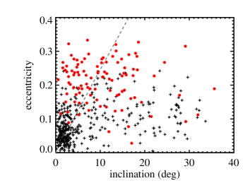
Figure 2.— Eccentricity vs. inclination with respect to the invariable plane for observed classical KBOs (black crosses) and 3:2 resonant KBOs (red circles) from the MPC catalog. The eccentricities of 3:2 resonant KBOs are systematically higher than the eccentricities of classical KBOs and do not correlate with inclination. This pattern is consistent with migration-induced eccentricity excitation, which does not affect inclination. Because 3:2 objects are more stable than classical bodies at high eccentricity, this pattern is also consistent with removal of high $e$ classical objects due to planet scattering, as occurs, for example, in chaotic capture. We include for reference the line $e=\sqrt{2}\sin(i)$, representing equipartition excitation of eccentricity and inclination.

As mentioned in Section 1, 3:2 objects do not exhibit the same excess of low inclination bodies seen in the classical population. This lack of a large cold population is potentially problematic in the context of migration-induced capture, but is not conclusive because the 3:2 resonance did not sweep through the region of the classical belt. However, among hot objects, the distribution of eccentricity and inclination mimics that expected for migration-induced capture. The inclinations of KBOs in the 3:2 resonance are not correlated with eccentricity and span the same range as the inclinations of hot classical objects. At the same time, the eccentricities of the resonant KBOs are systematically higher than those of the classical objects. This pattern of similar inclinations but offset eccentricities is consistent with migration-induced capture, which excites eccentricities while leaving inclinations largely unchanged. This pattern is suggestive but not conclusive evidence for migration-induced capture because high eccentricity KBOs are more stable in the 3:2 resonance than in the classical belt, and the observed eccentricity offset could alternatively result from the removal of high $e$ classical bodies.

4. BINARY FORMATION AS A FUNCTION OF SEMI-MAJOR AXIS

Having established that under the migration-induced capture scenario, we can statistically recover the the initial semi-major axes of KBOs in mean motion resonance with Neptune, we now show that the binary fractions of different populations of KBOs are expected to be a function of the locations in the protoplanetary disk at which those populations formed. In Section 4.1, we review proposed binary formation scenarios. We argue that binary formation mediated by dynamical friction with small bodies, as proposed by Goldreich et al. (2002), likely formed the Kuiper belt binaries. In Section 4.2, we review the Goldreich et al. (2002) formation mechanism, and in Section 4.3, we calculate the binary fraction as a function of formation distance. We note that other binary formation mechanisms which vary with distance could also generate an observable, though different, signature in the resonant population.

4.1. Binary Formation Scenarios

High mass-ratio binaries in the Kuiper belt, including Pluto/Charon, likely formed in collisions (McKinnon, 1989). However, the majority of observed binary KBOs are roughly equal-mass, wide-separation binaries (Noll et al., 2008b) that have too much angular momentum to be formed by the same mechanism. Motivated by this challenge, a series of new binary formation scenarios was proposed (e.g. Weidenschilling, 2002; Goldreich et al., 2002; Funato et al., 2004; Astakhov et al., 2005; Lee et al., 2007; Nesvorný et al., 2010). Most of these scenarios appeal to interactions within the Hill sphere, the region interior to the Hill radius of a KBO. The Hill radius denotes the distance from a KBO at which the tidal forces from the Sun and the gravitational force from the KBO, both acting on a test particle, are in equilibrium. It is given by

$$R_{H}\equiv a\left(\frac{m}{3M_{*}}\right)^{1/3}$$ (5)

where $a$ is the semi-major axis of the KBO and $m$ its mass. Weidenschilling (2002) proposed a collision between two KBOs inside the Hill sphere of a third. However, in the Kuiper belt, gravitational scattering between the two intruders is about 100 times more common than a collision. Binary formation by three body gravitational deflection ($L^{3}$ mechanism), as proposed by Goldreich et al. (2002), should therefore dominate over such a collisional formation scenario. A second binary formation scenario proposed by Goldreich et al. (2002) consists of the formation of a transient binary, which becomes bound with the aid of dynamical friction from the surrounding sea of small bodies ($L^{2}_{s}$ mechanism, §4.2). Schlichting & Sari (2008a) demonstrated that at the distance of the Kuiper belt, $L^{2}_{s}$ dominates over $L^{3}$. Astakhov et al. (2005) and Lee et al. (2007) suggest that transient binaries that spend a long time in their mutual Hill sphere, near a periodic orbit, form the binaries in the $L^{2}_{s}$ and $L^{3}$ mechanisms. Schlichting & Sari (2008a) investigated the relative importance of these long-lived transient binaries. They found that such transient binaries are not important for binary formation via the $L^{3}$ mechanism and that they become important only for very weak dynamical friction in the $L^{2}s$ mechanism. Funato et al. (2004) proposed a binary formation mechanism which involves a collision between two large KBOs that creates a small moon. An exchange reaction replaces the moon with a massive body with high eccentricity and large semi-major axis.

Finally, Nesvorný et al. (2010) suggested that Kuiper belt binaries could form directly during a gravitational collapse that leads to the formation of 100-km-sized KBOs. This binary formation scenario is fundamentally different in the sense that it assumes, based on recent work on the streaming instability (Youdin & Goodman, 2005; Johansen et al., 2007), that 100-km sized KBOs formed by direct gravitational collapse rather than coagulation. Whether such a gravitational collapse KBO formation scenario is feasible and whether it can explain the observed KBO size distribution, which is well matched by coagulation simulations (Kenyon & Luu, 1999; Kenyon, 2002; Kenyon & Bromley, 2004), remains to be determined. Furthermore, a gravitational collapse binary formation scenario, would have to provide a convincing explanation for the large binary fraction of similar brightness systems in the Kuiper belt and the absence of such binaries in the Asteroid belt. Nesvorný et al. (2010) appeal to enhanced binary disruption in the Asteroid belt due to collisions and scattering events to explain this difference. A dynamical origin, which is common in all the other binary formation scenarios discussed above, takes advantage of the fact that the Hill radius is more than an order of magnitude larger for KBOs compared to similar sized objects in the Asteroid belt. Gravitational capture binary formation scenarios therfore support the observations that the Kuiper belt is the ideal place for wide, similar brightness binaries to form.

We decided to focus on the Goldreich et al. (2002) binary formation mechanism for the calculations in this paper. Our choice is motivated by the success this binary formation scenario has had in explaining the binary abundance and the observed binary separation distribution. It also predicts the existence of triplet systems. The first triplet system was reported recently by Benecchi et al. (2010). One set of observations that are not successfully explained by the Goldreich et al. (2002) formation scenario is the mutual binary inclination distribution (Noll et al., 2008a). Binary formation rates are extremely sensitive to the velocity dispersion $v\sim\left<e\right>\Omega a$ of the population of large planetesimals from which they form, where $\left<e\right>$ is the typical eccentricity of a planetesimal. Efficient binary formation requires that the large KBOs have a velocity dispersion that is less than their Hill velocity, $v_{H}=\Omega R_{H}$. Binary formation rates quickly exceed the age of the solar system, once the velocity dispersion grows significantly above $v_{H}$ (Noll et al., 2008a; Schlichting & Sari, 2008a). Binary formation while sub-Hill velocities prevailed, however, predicts low mutual binary inclinations (Chiang et al., 2007; Schlichting & Sari, 2008b) and is inconsistent with the roughly uniform inclination distribution that is observed (see Naoz et al. (2010) and references theirin). Evolution of the mutual binary inclination after formation provides a possible solution to this problem. Although it has, for example, been suggested that the Kozai mechanism could affect the orbital evolution of Kuiper belt binaries (Perets & Naoz, 2009), it remains a topic of ongoing research if mutual binary inclinations can be excited to sufficiently large values that would allow such a mechanism to operate.

4.2. Binary Capture Mediated by Dynamical Friction

After specifying our assumptions, we now review the binary formation rate for the $L^{2}s$ mechanism. which will be useful in calculating the expected binary fraction. Following Goldreich et al. (2002), we use the “two-group approximation”, which consists of the identification of two groups of objects, small ones, that contain most of the total mass with surface mass density $\sigma$, and large ones, that contain only a small fraction of the total mass with surface mass density $\Sigma\ll\sigma$. We assume that $\sigma\sim\sigma_{40}(a/40~{}AU)^{\gamma}$ which is a generalization of the minimum-mass solar nebula (Weidenschilling, 1977; Hayashi, 1981), where $\sigma_{40}\sim 0.3\;\rm{g~{}cm^{-2}}$ is the surface density at a heliocentric distance of $40\rm{AU}$. The power-law index $\gamma$ is typically assumed to have values between -1 and -1.5, with submillimeter observations of the outer regions of protoplanetary disks favoring $\gamma\approx-1$ (Andrews et al., 2009).

We likewise parameterize the mass surface density of large bodies with sizes of $R\sim 100~{}\rm{km}$ and larger as $\Sigma\sim\Sigma_{40}(a/40~{}AU)^{\beta}$, where we treat $\beta$ as a free parameter. Estimates from Kuiper belt surveys (e.g., Trujillo et al., 2001; Trujillo & Brown, 2003; Petit et al., 2008b; Fraser & Kavelaars, 2009; Fuentes et al., 2009) yield $\Sigma_{40}\sim 3\times 10^{-4}\;\rm{g~{}cm^{-2}}$ in the current belt.

Goldreich et al. (2002) demonstrate that, under the assumption that $\Sigma$ was the same as it is now during the formation of Kuiper belt binaries, the velocity dispersion $v$ of $\sim$$100\rm{km}$ KBOs is damped by dynamical friction from the sea of small bodies such that $v<v_{H}$. This is referred to as the “shear-dominated velocity regime” because under these conditions, the relative velocity of two large bodies that encounter one another is dominated by their Keplerian shear. Binary formation is inefficient when $v\gtrsim v_{H}$ (Chiang et al., 2007; Schlichting & Sari, 2008b).

In particular, in this scenario, large bodies grow by the accretion of small bodies. Large KBOs viscously stir the small bodies. This stirring increases the small bodies’ velocity dispersion, $u$, which grows on the same timescale as $R$ and is given by

$$\frac{u}{v_{H}}\sim\left(\frac{\Sigma}{\sigma\alpha}\right)^{1/2}\sim 3\left(\frac{a}{40~{}AU}\right)^{(\beta-\gamma+1)/2}$$ (6)

where $\alpha=R/R_{H}$ (Goldreich et al., 2002). Meanwhile, the velocity $v$ of large KBOs increases due to mutual viscous stirring, but is damped by dynamical friction from the sea of small bodies such that $v<u$. Balancing the stirring and damping rates of $v$ and substituting for $u$ from Equation 6, we find

$$\frac{v}{v_{H}}\sim\alpha^{-2}\left(\frac{\Sigma}{\sigma}\right)^{3}\sim 0.1\left(\frac{a}{40~{}AU}\right)^{3(\beta-\gamma)+2}.$$ (7)

A transient binary forms when two large KBOs penetrate each other’s Hill sphere. This transient binary must lose energy in order to become gravitationally bound. In the $L^{2}_{s}$ mechanism, the excess energy is carried away by dynamical friction with the sea of small bodies. Since it is not feasible to examine the interactions with each small body individually, their net effect is modeled by an averaged force which acts to damp the large KBOs’ non-circular velocity. We parameterize the strength of this damping by a dimensionless quantity $D$ defined as the fractional decrease in non-circular velocity due to dynamical friction over time $\Omega^{-1}$:

$$D\sim\frac{\sigma}{\rho R}\left(\frac{u}{v_{H}}\right)^{-4}\alpha^{-2}\sim\frac{\Sigma}{\rho R}\alpha^{-2}\left(\frac{v}{v_{H}}\right)^{-1}\;\;,$$ (8)

where $\rho\approx 1$ g/cm³ is the internal density of a KBO. The first expression is an estimate of dynamical friction by the sea of small bodies for $u>v_{H}$. The second expression describes the mutual excitation among the large KBOs for $v<v_{H}$. These two expressions can be equated since the stirring among the large KBOs is balanced by the damping due to dynamical friction. Using this parameterization for the dynamical friction, the binary formation rate for equal mass bodies via the $L^{2}s$ mechanism in the shear-dominated velocity regime is given by

$$FR_{L^{2}s}=A_{L^{2}s}D\left(\frac{\Sigma}{\rho R}\right)\alpha^{-2}\Omega$$ (9)

(Goldreich et al., 2002) where $A_{L^{2}s}$ is a constant with a value of about 1.4 (Schlichting & Sari, 2008a). $FR_{L^{2}s}\sim 1.3\times 10^{-5}\rm{yr^{-1}}$ when evaluated at 40 AU.

4.3. Binary abundances

We now calculate the expected variation in the fraction of binaries formed as a function of semi-major axis. The binary separation, $s$, shrinks due to dynamical friction at a rate $s^{-1}|ds/dt|$. The probability of finding a large KBO in a binary per logarithmic band in $s$ is given by

$$s~{}p(s)\sim\frac{FR_{L^{2}s}}{s^{-1}|ds/dt|}$$ (10)

where $p(s)$ is the probability density of finding a large KBO in a binary with binary semi-major axis $s$. There are two regimes in binary separation that need to be considered separately. In the first regime the binary semi-major axis is sufficiently large such that the velocity of the binary components around their common center of mass, $v_{B}$, is small compared to the velocity dispersion of the small bodies that provide the dynamical friction, i.e. $v_{B}<u$. In this case $s^{-1}|ds/dt|=D$, given by Equation (8). However this regime only applies to binary semi-major axes that satisfy $GM/u^{2}<s<R_{H}$ which translates into binary angular separations of 3” and greater at heliocentric distances of about 40 AU. To our knowledge, only one (2001 QW322, Petit et al., 2009) out of about 70 currently known KBO binaries satisfies this criterion. We therefore focus from here onwards on the second regime for which $v_{B}>u$, which applies to binaries with angular separation of less than about 3” at a distances of about 40 AU. In this regime, the binary separation shrinks due to dynamical friction at a rate

$$\frac{1}{s}\left|\frac{ds}{dt}\right|\sim\frac{\sigma}{\rho R}\left(\frac{u}{v_{H}}\right)^{-2}\left(\frac{v_{B}}{v_{H}}\right)^{-2}\alpha^{-2}\Omega.$$ (11)

Substituting the above expression and the binary formation rate from Equation (9) into Equation (10) we find

$$s~{}p(s)\sim\frac{\Sigma}{\rho R}\left(\frac{u}{v_{B}}\right)^{-2}\alpha^{-2}\sim\frac{\sigma}{\rho R}\left(\frac{R}{s}\right)\alpha^{-2}$$ (12)

where in the last step, we used the expression for $u$ given in Equation (6) (Goldreich et al., 2002). The only semi-major axis dependence that enters in Equation (12) results from $\sigma$ and $\alpha$. For $\sigma\propto a^{\gamma}$ the binary fraction as a function of $a$ is given by

$$s~{}p(s)\sim\frac{\sigma}{\rho R}\left(\frac{R}{s}\right)\alpha^{-2}\propto a^{\gamma+2}$$ (13)

at the time of formation.

Equations (12) and (13) show that the binary fraction does not explicitely depend on $\Sigma$. We also note that, because we are interested in the scaling of $s~{}p(s)$ with $a$, the values of $\sigma_{40}$ and $\Sigma_{40}$ do not matter as long as their ratio is such that binary formation can proceed in the shear dominated velocity regime. Given everything else equal, we find that the binary fraction is between 1.4 times ($\gamma=-3/2$) to twice ($\gamma=-1$) as high at 50 AU compared to 25 AU during the epoch of binary formation. This trend in the binary fraction as a function of heliocentric distance is in agreement with observations that find a binary fraction that is more than a factor of 2 lower in the excited and hot classical populations, which most likely formed closer to the Sun and were scattered to their current locations, than in the cold classical population, which most likely formed in-situ at about 40 AU. An analogous calculation for the $L^{3}$ mechanism of binary formation yields the scaling relation $s~{}p(s)\propto a^{\gamma-1/4}$, where we used $\Sigma/\sigma\sim\alpha^{3/4}$ (Schlichting & Sari, 2011).

In Section 5, we explore the expected binary fraction as a function of current dynamical class in more detail. We recall here that the power-law index of the small bodies’ mass surface density, $\gamma$, is uncertain. Often $\gamma=-1.5$ is used based on the minimum mass solar nebula (Hayashi, 1981), but protoplanetary disk observations at distances comparable to the Kuiper belt (Andrews et al., 2009) suggest $\gamma=-1$. In the calculations that follow, we assume $\gamma=-1$. If $\gamma=-1.5$ then the trends in the binary abundance will still be present but smaller in magnitude. Particle pile-ups (e.g., Youdin & Chiang, 2004), if they occur, result in a shallower mass surface density profile, making trends in binary abundance more pronounced.

Finally, as mentioned above, efficient binary formation (as proposed by Weidenschilling (2002); Goldreich et al. (2002); Funato et al. (2004); Astakhov et al. (2005); Lee et al. (2007)) requires $v\lesssim v_{H}$, which implies that the velocity dispersion of the large bodies that form binaries has to be damped to sub Hill velocities. If this damping is provided by dynamical friction generated by small bodies, as we have assumed in deriving Equation (7), than this implies that $\Sigma\ll\sigma$, because $v>v_{H}$ otherwise. These binary formation scenarios are therefore inconsistent with reduction of the mass in the Kuiper-belt by two orders of magnitude or more in an entirely size-independent fashion, for example in one large scattering event. Analytic work and numerical coagulation simulations that model the growth of KBOs indeed find that only about $\alpha^{3/4}\sim 10^{-3}$ of the initial disk mass is converted into large KBOs suggesting that $\Sigma/\sigma\sim 10^{-3}$ (Kenyon & Luu, 1999; Kenyon & Bromley, 2004; Schlichting & Sari, 2011), which is consistent with the surface density values used in this section and the conclusion that $v<v_{H}$.

5. KBO BINARY FRACTIONS AS A FUNCTION OF DYNAMICAL CLASS

In order to test the nature of Neptune’s migration with the abundance of comparable-mass, wide-separation KBO binaries, we suggest the following procedure. We recall that we are searching for a signature of an outer solar system history in which the cold (low inclination) classical population formed in situ, the hot (high inclination population) formed closer to the Sun and was dynamically mixed during transport to its current location, and resonant KBOs are a superposition of these two populations, caught into resonance during migration of Neptune spanning between several and $\sim$10 AU (§2). Our proposed signature of this class of migration histories is summarized in Figure 3.

5.1. Looking for a Cold Component

First one needs to establish whether a low inclination component, analogous to the cold classical population, exists in a given resonant population. Recall that because any hot population will contain low-inclination bodies, a cold component refers not merely to objects with low-inclinations but rather to a separate low-inclination population. As yet, for the 3:2 there is no dynamical evidence for two inclination components, implying that if one exists it is less pronounced than in the classical belt, and insufficient data is available for the 2:1 resonance to make this determination (Gulbis et al., 2010). We note that because 3:2 resonant KBOs originated in a different location in the disk than classical KBOs if migration-induced capture occurred, and because the inclinations of resonant bodies evolve more over long-term integrations than their classical counterparts (Volk & Malhotra, in prep.), the characteristic inclination that divides the low and high inclination populations in the 3:2 resonance could be different from that in the classical belt. Furthermore, this characteristic inclination could vary between resonances. If a resonance does contain a cold component with a broader width or a smaller relative contribution than seen in the classical belt, it should be observable in binaries, just as the cold component can be picked out just from the binary fraction in the classical belt (Noll et al., 2008b). We therefore suggest searching for a cold component by comparing the binary fractions of low and high inclination objects in a given resonance. We discuss this distinction in the context of KBO colors and sizes in Section 6.

Theoretically, if cold and hot components are present in a resonance, our schematic migration scenario predicts fewer binaries in the high inclination population. This is both because they originated closer to the Sun and because the excitation process may have broken binaries that were originally there. Parker & Kavelaars (2010) have shown numerically that binary disruption is common for objects transported across the semi-major axis of Neptune. They consider the particular chaotic capture scenario modeled in Levison et al. (2008) in which all KBOs, including those ultimately on low eccentricity and low inclination orbits, begin interior to the current cold classical belt, and they find that wide binaries are efficiently destroyed. This finding is in conflict with the observed large binary fraction in the cold classical belt (Noll et al., 2008a). Parker & Kavelaars (2010) argue that the difference in binary fraction between the cold and hot classicals may reflect scattering of the hot classicals off of Neptune during their history, contrasted with a gentler dynamical history for low inclination objects, which formed exterior to Neptune and never encountered the planet. Depending on the details of the as yet unknown process exciting inclinations in the Kuiper belt, there may be trends with inclination in the binary fraction of the high inclination population. Nevertheless, we expect the overall fraction to be smaller than that in the low inclination population.

A lack of a cold component in the 3:2 resonance might be explained in the context of migration-induced capture if the original disk was substantially excited interior to the current location of the 3:2, though no proposed model currently produces such excitation. In contrast, a lack of a cold component in the 2:1 resonance would seriously challenge a scenario invoking smooth migration through a hot plus cold planetesimal disk because the 2:1 resonance should have swept through the location of the current cold classical belt.

We emphasize that the 3:2 and 2:1 resonances are the best locations to test for the presence of a cold component. Higher order resonances preferentially capture objects with large eccentricities. Therefore, if eccentricities and inclinations are correlated, higher order resonances may only contain hot components even if they swept through a disk that had a cold component. However, if a higher order resonance does have a population of low inclination objects, it should also have a higher binary fraction in the cold component compared to the hot component.

5.2. Looking for Trends in the Low Inclination Resonant Population

Provided that a cold component can be established in a Kuiper belt resonance (Section 5.1), we suggest looking for the following trends in binary fraction within the low inclination resonant population. First, we propose looking for differences across the binary fractions of the cold populations of different resonances and of the cold classical belt, and second we propose looking for trends in binary fraction with eccentricity within the low inclination population of a single resonance. Because it requires observations for fewer objects per resonance, the former effect may be easier to measure, and we describe it first.

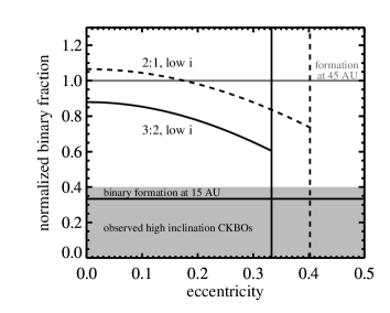
Figure 3.— Fraction of low-inclination, resonant Kuiper belt objects predicted to be wide-separation, roughly equal-mass binaries, under the hypothesis that Neptune captured objects into resonance as it migrated $\sim$10 AU. We normalize this expected fraction to the binary fraction among low-inclination (cold) classical objects (CKBOs) at 45 AU. The vertical lines show both the maximum eccentricity excitation from migration by 9.4 AU (calculated using Equation 2) and the maximum observed eccentricities in 3:2 and 2:1 resonances. The agreement of these values is promising for the migration scenario, but chaos at large eccentricities might also explain the different maximum eccentricities in different resonances. The observed binary fraction among highly inclined (hot) CKBOs (shaded region) is consistent with formation $\lesssim$15 AU from the Sun, though scattering events could disrupt binaries, complicating this interpretation.

Figure 3 displays the binary fraction as a function of eccentricity for low inclination objects in the 3:2 and 2:1 resonances, normalized to the binary fraction of cold classical KBOs at 45 AU. These relative fractions are calculated by combining the expected formation locations of the resonant KBOs from Equation (4) with the trend in binary formation rate as a function of formation location given by Equation (13) and $\gamma=-1$. The difference between true and expected formation location is discussed in Section 3.2.

In general, the larger the semi-major axis of a resonance, the higher the binary fraction of its cold component should be. To zeroth order, we expect the binary fraction in the 2:1 resonance to be roughly comparable to the cold classicals. A higher fraction of large eccentricity objects in resonance would lower this estimate, as can be seen from Figure 3. To correct for this bias in a given observed sample, one could, for example, calculate the estimated fraction using the eccentricity of each observed object from Figure 3 and calculate the average. In contrast, we expect cold 3:2 objects to have a 20–30% lower binary fraction than the cold classicals. Again, for a particular set of observations, one can calculate an expected fraction as above.

Uncertainties in the population statistics of resonant KBOs prevent us from making a robust estimate of the number of measurements required to distinguish this effect. Nevertheless, we provide the likely scale of the observations required by calculating the following example. If the binary fraction of cold classicals at 45 AU is $\sim$30%, consistent with the observed binary fraction among cold CKBOs (Noll et al., 2008b), then averaged over all eccentricities, the low inclination 3:2 objects are predicted to have binary fraction $\sim$0.22, compared with $\sim$0.27 in the 2:1 resonance and $\sim$0.29 in the cold classical belt. Identifying such subtle differences would require measuring the fraction of each population to within approximately 2–3%. Noll et al. (2008b) measure a binary fraction of $29^{+7}_{-6}$% in the cold classicals based on binary detection for 17 of 58 targets. We estimate that a sample containing approximately $N\sim 250$ objects would generate errors of $\sqrt{0.3N}/N=0.035$, enough to distinguish our predicted binary fractions for cold 3:2 objects from the cold classicals. This approximate number of observations would be required in each population. The binary fractions in the cold 3:2 and cold 2:1 resonant populations could be separated with samples of $\sim$500 objects each.

Currently, only 101 3:2 objects are known (as defined in §3.2), 54 of which have $i<10^{\circ}$ and 26 of which have $i<5^{\circ}$. In the 2:1 resonance, 15 objects are known, 9 of which have $i<10^{\circ}$ and 6 of which have $i<5^{\circ}$. However, according to Kavelaars et al. (2009), approximately $2.5^{+2.5}_{-1.2}\times 10^{4}$ Plutinos are present in the belt with solar system absolute magnitude in the $g^{\prime}$ filter of $H_{g}<10$. Given

$$D(\rm km)=2\times 1.5\times 10^{8}p^{-0.5}10^{0.2(m_{\odot}-H)}$$ (14)

(e.g., Petit et al., 2008a) with $m_{\odot}=-26.47$ in $g^{\prime}$ (Kavelaars et al., 2009), $H=H_{g}<10$ corresponds to diameters $D>50$ km. We have used albedo $p=0.1$, consistent with observed KBOs in the visible (Brucker et al., 2009).

We are interested in objects near the break in the KBO size distribution, corresponding to the largest number of KBOs that are not likely to have collisionally evolved over the age of the solar system. This break is measured at apparent magnitude $\sim 25$ in $R$-band (Fuentes et al., 2009). At a distance $d$ from the Sun, an object with absolute magnitude $H$ has apparent magnitude $H+2.5\log(d^{2}\Delta^{2}/{\rm AU}^{4})$, with $\Delta\approx d-1$ AU. Using $d=42$ AU and $m_{\odot}=-27.12$ (appropriate for the Bessel R filter), the break is at $D\sim 60$km. This differs from the 90 km diameter quoted in Fuentes et al. (2009) due to our larger assumed albedo. The actual diameter at the break is uncertain to within approximately a factor of 2. Since $D\sim 50$km equals the size at the break to within the errors, we conservatively adopt a number of Plutinos equal to half of the estimated number of Plutinos with $H_{g}<10$. Given these assumptions, if a cold population of 3:2 KBOs is shown to exist with $i<10^{\circ}$ and if the fraction of Plutinos with $i<10^{\circ}$ is $\sim$0.5 as in the currently observed sample, then the 3:2 population likely contains at least $\sim$$6\times 10^{3}$ dynamically cold objects larger than the break in the size distribution. More than an order of magnitude more Plutinos are likely present in the belt than would be required to compare the binary fractions of cold 3:2 objects and cold classicals.

The number of objects in the 2:1 resonance is less well constrained than the number in the 3:2 resonance. Chiang & Jordan (2002) estimate that the 2:1 hosts a factor of $\sim$3 fewer objects than the 3:2, and Lawler et al. (in prep.) estimate a factor of $\sim$4 fewer objects in the 2:1 than in the 3:2 based on the well-characterized Canada-France Ecliptic Plane Survey. Given a factor of 4 reduction and assuming, in analogy with the 3:2, that half of the 2:1 objects are members of a cold population, a factor of $\sim$3 more 2:1 objects are present than we predict are required to differentiate between the binary fractions of the cold 3:2 and 2:1 populations.

LSST is currently projected to detect more than 30,000 KBOs with diameters larger than $\sim$100 km (Ivezic et al., 2008). Using $m_{\odot}=-27.08$ (SDSS $r^{\prime}$ filter) and albedo $p=0.1$, the LSST limiting magnitude of $\sim 24.5$ in $r$-band corresponds to KBOs with diameters $D\gtrsim$ 70 km at the semi-major axis of the 3:2 resonance ($d\approx 39$ AU) and $D\gtrsim 100$ km at the semi-major axis of the 2:1 resonance ($d\approx 48$ AU). In practice, smaller resonant KBOs will be observable because the large eccentricities of these objects bring them closer to the Sun. With an angular resolution of $\sim$0.7” (Ivezic et al., 2008), LSST will likely be able to distinguish some wide-separation binaries without requiring follow-up observations. However, the observations in Noll et al. (2008b) using the Hubble Space Telescope have a factor of 10 better resolution and include binaries that will not be resolved by LSST. Kavelaars et al. (2009) estimate that Plutinos are $\sim$20% as abundant as CKBOs. If only $\sim$2% or more of the objects discovered by LSST are Plutinos and if the fraction of wide binaries among these objects is measured, then LSST will detect sufficiently many low inclination Plutinos to search for our predicted difference between the binary fractions of cold 3:2 and cold classical objects.

LSST may also detect the $\sim$500 low inclination 2:1 objects required to differentiate between the 3:2 and 2:1 populations. Conservatively choosing a size distribution $dN/dR\propto R^{-q}$ with $q=5$ (at the large end of the $q=2$–5 range measured for various subpopulations of the belt, Fuentes et al., 2009; Fraser & Kavelaars, 2009; Fraser et al., 2010), we estimate the number of cold 2:1 objects with $D\sim 100$km to be $\sim$200. These objects will be observable by LSST at their semi-major axis. A KBO in 2:1 resonance with $e=0.2$ spends $\sim$16% of its time at distances from the Sun of no more than 40 AU. At these distances, objects with $D\sim 70$ km will be visible, adding another $\sim 800\times 0.16\sim 100$ observable low-inclination bodies, for a total of $\sim$300 objects. Given the substantial uncertainties encompassed in this calculation and our conservative choice of $q=5$, it is plausible that LSST will detect sufficient low inclination 2:1 bodies to differentiate between the cold 3:2 and 2:1 populations.

We now turn to the search for trends in binary fraction with eccentricity within the low inclination population of a single resonance. As illustrated in Figure 3, within a single resonance, the binary fraction at small eccentricities is $\sim$40% larger than that at the highest observed eccentricities. If we consider the average of all objects with $e<0.2$ compared with those having $e\geq 0.2$, the difference is reduced to $\sim$20%, though this value depends on the distribution of eccentricities included in the average.

Extending our example calculation above, we estimate that low inclination 3:2 objects have binary fraction $\sim$0.25 for $e<0.2$ and $\sim$0.21 for $e\geq 0.2$. These fractions could be separated with samples of $N\sim 750$ in each of the $e<0.2$ and $e\geq 0.2$ subsets of the low-inclination data. Again, these numbers depend on the distribution of eccentricities of the objects in the resonances. Though the observational effort needed would be substantial, this experiment should be possible using KBOs discovered by LSST. An order of magnitude more objects are likely present in the belt than would be required to test this effect, and LSST will detect a sufficient number of Plutinos to search for our predicted trend if $\sim$10% or more of its projected KBO discoveries are in the 3:2 resonance.

In our example, the low inclination 2:1 objects are predicted to have binary fraction $\sim$0.31 for $e<0.2$ and $\sim$0.26 for $e\geq 0.2$. Separation of these fractions requires $\sim$1000 low-inclination 2:1 objects, equally divided between low and high eccentricities. We estimate that enough objects exist in the belt to perform this experiment. Though our estimate indicates that LSST will discover a factor of $\sim$3 fewer 2:1 KBOs than required, we emphasize that this calculation employs a conservative size distribution and is highly uncertain because the intrinsic population of 100 km objects in the 2:1 resonance is not well known.

We recall that because, in the migration scenario, the 2:1 resonance passed through the cold classical belt, the 2:1 resonance should provide the clearest case for our dynamical signature. If the 3:2 resonance has a cold component, then it should also provide a good case for testing the binary abundance. As mentioned above, higher order resonances are less likely to capture unexcited objects. However, if they have some cold component, then they should show a similar trend in the binary abundance as a function of eccentricity as the 3:2 and 2:1 resonances.

We re-emphasize that these trends should only exist among an observed cold (low-inclination) component of the resonant population, if such a component exists. We further emphasize that we propose to test the binary fraction and not the absolute number of binaries in the resonant populations. Long-term differences in the loss rates from different resonances or as a function of orbital parameters within any given resonance (e.g., Tiscareno & Malhotra, 2009) will not affect our results because these losses should affect binaries and single KBOs equally. Finally, we note that the KBOs need to be tightly in resonance (small libration angle) rather than tenuously in resonance, since they may otherwise have been transiently captured by scattering (Lykawka & Mukai, 2006).

5.3. Interpretation for Different Dynamical Sculpting Models

If a cold component is observed in the fraction of wide-separation, comparable mass binaries in one or more resonances, it will provide support for migration-induced capture, which naturally produces a cold component within resonances. Migration-induced capture may be consistent with no cold component in the 3:2 resonance, but the lack of a cold component in the 2:1 resonance would argue strongly against this model. In contrast, in chaotic capture as envisioned by Levison et al. (2008), the binary fraction in the resonances should match the fraction in the scattered disk, even at low inclinations. Given the presence of a distinct binary fraction in the cold classical disk, for chaotic capture to be viable, the models presented in Levison et al. (2008) need to be adjusted to allow maintenance of a cold classical population that formed in situ. Even if such a modification is possible, it would not generate a cold component within the resonances, retaining the search for a cold resonant component as a useful distinguishing test.

Measurement of a trend in binary fraction with eccentricity within the cold component of a resonance would provide conclusive evidence of migration-induced capture. Unfortunately, lack of such a trend would not constitute conclusive evidence that migration-induced capture did not occur. We expect such a trend to be a subtle effect, and uncertainty in the surface-density profile of the initial disk means that we cannot conclusively predict its magnitude. Lack of an observed trend could imply a steeper surface density (nearer $\gamma=-2$) or a different binary formation scenario. Similarly, if a trend in binary fraction with eccentricity is observed among low-inclination resonant KBOs, but the trend differs from our prediction, this could imply either a different surface density profile or an alternative binary formation mechanism.

6. KBO COLORS AND SIZES

Binary fraction is not the only physical characteristic that has been shown to differ between dynamical populations in the Kuiper belt—striking correlations with KBO inclination have also been measured for KBO colors (Tegler & Romanishin, 2000; Trujillo & Brown, 2002; Peixinho et al., 2008) and sizes (Levison & Stern, 2001). These characteristics are more difficult to interpret than the binary fraction because no quantitative theory exists for how they should vary as a function of formation location. Nevertheless, we now consider the procedure outlined in Section 5 in light of these properties. We address the 3:2 resonance, where data is most abundant. A detailed reassessment of the available data is warranted but beyond the scope of this paper. For our purposes, we demonstrate that currently measured size and color distributions, as compiled by (Almeida et al., 2009) for 3:2 objects and by (Peixinho et al., 2008) for classical objects, do not conclusively distinguish between our two dynamical scenarios.

First, does the 3:2 resonance contain a cold component? Figures 4 (a) and (b) display KBO diameters and B-R colors as a function of inclination for objects in the 3:2 resonance and for classical objects. We convert inclinations to be with respect to the invariable plane. We calculate diameters from the absolute solar system magnitudes $H_{R}$ quoted in Almeida et al. (2009) and Peixinho et al. (2008) using Equation (14) with $H=H_{R}$ and $m_{\odot}=-27.12$ (Bessel $R$ filter). In keeping with the high albedos observed for KBOs in the visible (Brucker et al., 2009), we use albedo $p=0.1$. Members of the Haumea collisional family (Brown et al., 2007; Ragozzine & Brown, 2007; Snodgrass et al., 2010) are marked.

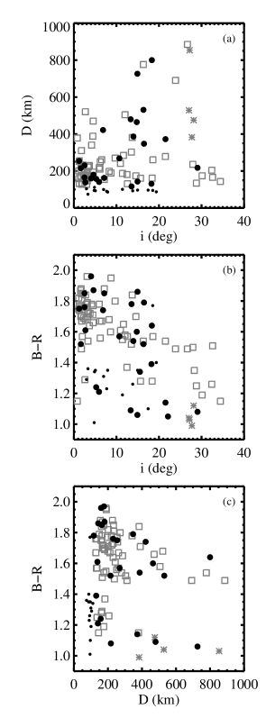
Figure 4.— Observed diameter as a function of inclination with respect to the invariable plane (a), inclination vs. B-R color (b), and diameter vs. B-R color (c) for classical (gray squares) and 3:2 resonant (black circles) KBOs. Small circles correspond to 3:2 objects with sizes smaller than the minimum-size classical KBO. Classical objects that are known members of the Haumea collisional family (gray asterisks) have unusually blue colors, known to result from water ice features. Data for resonant objects is compiled by Almeida et al. (2009) and that for classical KBOs is compiled by Peixinho et al. (2008). See the text for details of our conversion from magnitudes, $H_{R}$, to diameters.

Figure 4 (a) suggests that 3:2 objects with inclinations $<5$–10^∘ may have systematically smaller sizes than high inclination population, consistent with the trend seen among classical objects. At first glance, the color trend is less promising. However, as noted by Almeida et al. (2009), the smallest 3:2 resonant KBOs have systematically bluer colors than their larger compatriots (see Figure 4 (c)). The smallest classical object in the sample considered here has $D\sim 110$ km, close to the observed break in the classical size distribution (Fuentes et al., 2009). We suggest that this color difference, unlike the color variation among large KBOs, may result from a collisional break in the population of 3:2 objects that is not yet observed among classical KBOs because colors have not been measured for small enough objects. This possibility merits further investigation (Schlichting et al., in prep.). Almeida et al. (2009) alternatively suggest that this trend may come from collisions between Plutinos and Neptune Trojans. If either idea is validated, only the colors of those KBOs too large to suffer ongoing collisions reflect conditions in the initial nebula and only those should be considered when searching for a difference in color between in a low-inclination and a high-inclination population. Figure 4 (b) is suggestive, though certainly not conclusive, that such a difference exists, again divided by a characteristic inclination between 5 and 10^∘. This is similar to the color break that Peixinho et al. (2008) find at $\sim$$12^{\circ}$ in the classical belt. We highlight that the transition in physical properties could be at $\sim$$10^{\circ}$ or even higher rather than at $5^{\circ}$ as usually quoted, even in the classical belt.

Next, do 3:2 objects show a trend in size or color with eccentricity? No such trend has been observed in the 3:2 population (Doressoundiram et al., 2008). However, because no quantitative model exists for how large KBO colors vary with formation distance, it is not clear whether we would expect to see such a trend in colors. For example, the difference in color between cold and hot classicals might result not from a continuous variation in the protoplanetary nebula but rather from critical transitions in the ability of KBOs to incorporate or retain different ices (e.g., Schaller & Brown, 2007). In this case, the critical transition separating the region of formation for hot and cold CKBOs could have been interior to the region swept by the 3:2 resonance, leaving no trend with eccentricity in the colors of cold resonant objects. If such a trend does exist, we would expect higher eccentricity objects to have bluer colors. The number of large, low-inclination, 3:2 resonant objects is not large enough to determine whether this is the case.

7. SUMMARY

Observations demonstrate that unlike asteroids, a substantial fraction of Kuiper belt objects are comparable-mass, wide separation binaries (Noll et al., 2008a). These bodies typically have sizes of $\sim$100 km. Unlike the Pluto-Charon system and other large mass-ratio binaries, they likely formed by dynamical capture rather than through collisions. Because the Hill radius of a planetesimal increases with distance from the Sun, the efficiency of dynamical capture is higher for binaries that formed farther from the Sun.

The binary fraction in the cold classical Kuiper belt is $\sim$29%, compared with $\sim$10% for hot classical KBOs (Noll et al., 2008b). This discrepancy suggests that objects in the hot classical belt formed closer to the Sun where binary formation was less efficient. The binary fraction of the hot belt may also have been reduced by binary disruption during scattering interactions with Neptune (Parker & Kavelaars, 2010). In this paper, we have developed a method that uses the fraction of wide-separation, comparable mass binaries in various populations of the Kuiper belt to distinguish between two competing frameworks for the dynamical sculpting of the belt. If current projections are correct, we expect LSST to discover sufficiently many Kuiper belt objects to perform our proposed tests.

In both dynamical scenarios, during the late stages of planet formation, Neptune was located $\sim$10 AU or more closer to the Sun than its current semi-major axis of 30 AU. A dynamical cataclysm excited the the planet’s orbit, which was subsequently damped by dynamical friction with planetesimal debris. While Neptune’s orbit was excited, it interacted with and excited the orbits of nearby planetesimal debris. In this context, we consider the following two scenarios, named for the methods by which resonant KBOs are captured.

1. “Migration-induced capture.” Neptune’s orbit was damped onto an approximately circular, coplanar orbit while it still orbited $\sim$10 AU closer to the Sun than it does today. It then migrated smoothly outward to its current location as it scattered planetesimal debris (Fernandez & Ip, 1984), capturing KBOs into resonance as it proceeded (Malhotra, 1993, 1995). Each resonance captured objects from a distinct region of the protoplanetary disk, and the final eccentricity of a resonant KBO is correlated with the location of its capture into resonance.

2. “Chaotic capture.” Neptune scattered quickly onto an orbit at most a few AU away from its current location. The planet’s large eccentricity produced a chaotic region of overlapping resonances extending out to the 2:1 resonance, allowing objects scattered by Neptune to fill the region of space currently containing the Kuiper belt. Neptune’s eccentricity then damped, leaving objects in resonance (Levison et al., 2008). Due to the chaotic nature of this process, most or all information about the formation locations of KBOs was randomized.

To distinguish between these models, we calculate the fraction of wide-separation, roughly equal-mass binaries among KBOs with diameter $\sim$100 km expected for different dynamical populations under the hypothesis of migration-induced capture. We assume that KBO binaries formed via transient binary capture, made permanent by dynamical friction with small bodies (the $L^{2}s$ mechanism, Goldreich et al., 2002). We evaluate our expressions for binary formation in a disk with surface density profile $\sigma\propto a^{-1}$, consistent with observations of the outer regions of extrasolar protoplanetary disks (Andrews et al., 2009). Other binary formation mechanisms that vary with location in the protoplanetary disk and other disk surface density profiles will produce similar, but quantitatively different, signatures. In particular, the $L^{3}$ mechanism produces an opposite trend in the binary fraction with formation location compared to the $L^{2}s$ mechanism.

Figure 3 summarizes the pattern of binary fractions predicted as a result of migration-induced capture, given these choices. A low-inclination component of the 2:1 resonance should exist with a larger binary fraction than its high inclination component. Such a component may also exist in the 3:2 resonance. Among bodies with inclinations less than 5–10^∘, the fraction of binaries in the 2:1 resonance should be comparable to that in the classical belt, while the low-inclination component in the 3:2, if it exists, should have a fraction $\sim$20–30% lower than among classical KBOs. Within the low inclination component of the 3:2 or 2:1 resonance, objects with $e<0.2$ should have a binary fraction $\sim$20% higher than those with $e\gtrsim 0.2$. Our calculations are not affected by dynamical loss processes that operate with varying efficiency in different resonant populations (e.g., Tiscareno & Malhotra, 2009)—these processes affect single and binary KBOs equally and we are interested only in the binary fraction. Chaotic capture does not produce these signatures.

Though measurement of the full range of dynamical signatures predicted in this paper will require a substantial observational effort, searches for low-inclination components in the binary fractions of the 3:2 and 2:1 resonances are within immediate reach. When compared with the cold component observed in the classical belt, these cold resonant populations need not include the same fraction of the overall population, nor must they have the same characteristic inclination. Lack of a low inclination component in the 2:1 resonance would indicate that migration-induced capture is unlikely. Conversely, presence of a low inclination component in either resonance would constitute strong evidence for the migration-induced capture mechanism.

References

- Allen et al. (2002) Allen, R. L., Bernstein, G. M., & Malhotra, R. 2002, AJ, 124, 2949
- Almeida et al. (2009) Almeida, A. J. C., Peixinho, N., & Correia, A. C. M. 2009, A&A, 508, 1021
- Andrews et al. (2009) Andrews, S. M., Wilner, D. J., Hughes, A. M., Qi, C., & Dullemond, C. P. 2009, ApJ, 700, 1502
- Astakhov et al. (2005) Astakhov, S. A., Lee, E. A., & Farrelly, D. 2005, MNRAS, 360, 401
- Benecchi et al. (2010) Benecchi, S. D., Noll, K. S., Grundy, W. M., & Levison, H. F. 2010, Icarus, 207, 978
- Bernstein et al. (2004) Bernstein, G. M., Trilling, D. E., Allen, R. L., Brown, M. E., Holman, M., & Malhotra, R. 2004, AJ, 128, 1364
- Brouwer (1963) Brouwer, D. 1963, AJ, 68, 152
- Brown (2001) Brown, M. E. 2001, AJ, 121, 2804
- Brown et al. (2007) Brown, M. E., Barkume, K. M., Ragozzine, D., & Schaller, E. L. 2007, Nature, 446, 294
- Brown & Pan (2004) Brown, M. E. & Pan, M. 2004, AJ, 127, 2418
- Brucker et al. (2009) Brucker, M. J., Grundy, W. M., Stansberry, J. A., Spencer, J. R., Sheppard, S. S., Chiang, E. I., & Buie, M. W. 2009, Icarus, 201, 284
- Butler et al. (2006) Butler, R. P., Wright, J. T., Marcy, G. W., Fischer, D. A., Vogt, S. S., Tinney, C. G., Jones, H. R. A., Carter, B. D., Johnson, J. A., McCarthy, C., & Penny, A. J. 2006, ApJ, 646, 505
- Cameron & Ward (1976) Cameron, A. G. W. & Ward, W. R. 1976, in Lunar and Planetary Institute Conference Abstracts, Vol. 7, Lunar and Planetary Institute Conference Abstracts, 120–+
- Chambers (1999) Chambers, J. E. 1999, MNRAS, 304, 793
- Chiang & Choi (2008) Chiang, E. & Choi, H. 2008, AJ, 136, 350
- Chiang et al. (2007) Chiang, E., Lithwick, Y., Murray-Clay, R., Buie, M., Grundy, W., & Holman, M. 2007, in Protostars and Planets V, ed. B. Reipurth, D. Jewitt, & K. Keil (Tucson: University of Arizona Press), 895–911
- Chiang & Jordan (2002) Chiang, E. I. & Jordan, A. B. 2002, AJ, 124, 3430
- Chiang et al. (2003) Chiang, E. I., Jordan, A. B., Millis, R. L., Buie, M. W., Wasserman, L. H., Elliot, J. L., Kern, S. D., Trilling, D. E., Meech, K. J., & Wagner, R. M. 2003, AJ, 126, 430
- Doressoundiram et al. (2008) Doressoundiram, A., Boehnhardt, H., Tegler, S. C., & Trujillo, C. 2008, in The Solar System Beyond Neptune, ed. Barucci, M. A., Boehnhardt, H., Cruikshank, D. P., & Morbidelli, A. (Tucson: University of Arizona Press), 91–104
- Elliot et al. (2005) Elliot, J. L., Kern, S. D., Clancy, K. B., Gulbis, A. A. S., Millis, R. L., Buie, M. W., Wasserman, L. H., Chiang, E. I., Jordan, A. B., Trilling, D. E., & Meech, K. J. 2005, AJ, 129, 1117
- Fernandez & Ip (1984) Fernandez, J. A. & Ip, W.-H. 1984, Icarus, 58, 109
- Fraser et al. (2010) Fraser, W. C., Brown, M. E., & Schwamb, M. E. 2010, ArXiv e-prints, arXiv:1008.1058
- Fraser & Kavelaars (2009) Fraser, W. C. & Kavelaars, J. J. 2009, AJ, 137, 72
- Fuentes et al. (2009) Fuentes, C. I., George, M. R., & Holman, M. J. 2009, ApJ, 696, 91
- Fuentes & Holman (2008) Fuentes, C. I. & Holman, M. J. 2008, AJ, 136, 83
- Funato et al. (2004) Funato, Y., Makino, J., Hut, P., Kokubo, E., & Kinoshita, D. 2004, Nature, 427, 518
- Gladman et al. (2008) Gladman, B., Marsden, B. G., & Vanlaerhoven, C. 2008, in The Solar System Beyond Neptune, ed. Barucci, M. A., Boehnhardt, H., Cruikshank, D. P., & Morbidelli, A. (Tucson: University of Arizona Press), 43–57
- Goldreich et al. (2002) Goldreich, P., Lithwick, Y., & Sari, R. 2002, Nature, 420, 643
- Goldreich et al. (2004a) —. 2004a, ApJ, 614, 497
- Goldreich et al. (2004b) —. 2004b, ARA&A, 42, 549
- Gomes (2003) Gomes, R. S. 2003, Icarus, 161, 404
- Gomes et al. (2004) Gomes, R. S., Morbidelli, A., & Levison, H. F. 2004, Icarus, 170, 492
- Gulbis et al. (2010) Gulbis, A., Elliot, J., Adams, E., Benecchi, S., Buie, M., Trilling, D., & Wasserman, L. 2010, ArXiv e-prints
- Hahn & Malhotra (2005) Hahn, J. M. & Malhotra, R. 2005, AJ, 130, 2392
- Hartmann & Davis (1975) Hartmann, W. K. & Davis, D. R. 1975, Icarus, 24, 504
- Hayashi (1981) Hayashi, C. 1981, Progress of Theoretical Physics Supplement, 70, 35
- Ivezic et al. (2008) Ivezic, Z., Tyson, J. A., Allsman, R., Andrew, J., Angel, R., & for the LSST Collaboration. 2008, ArXiv e-prints, arXiv:0805.2366 v1.0
- Jewitt & Luu (1993) Jewitt, D. & Luu, J. 1993, Nature, 362, 730
- Jewitt et al. (1998) Jewitt, D., Luu, J., & Trujillo, C. 1998, AJ, 115, 2125
- Johansen et al. (2007) Johansen, A., Oishi, J. S., Mac Low, M., Klahr, H., Henning, T., & Youdin, A. 2007, Nature, 448, 1022
- Kavelaars et al. (2009) Kavelaars, J. J., Jones, R. L., Gladman, B. J., Petit, J., Parker, J. W., Van Laerhoven, C., Nicholson, P., Rousselot, P., Scholl, H., Mousis, O., Marsden, B., Benavidez, P., Bieryla, A., Campo Bagatin, A., Doressoundiram, A., Margot, J. L., Murray, I., & Veillet, C. 2009, AJ, 137, 4917
- Kenyon (2002) Kenyon, S. J. 2002, PASP, 114, 265
- Kenyon & Bromley (2004) Kenyon, S. J. & Bromley, B. C. 2004, AJ, 128, 1916
- Kenyon & Luu (1999) Kenyon, S. J. & Luu, J. X. 1999, AJ, 118, 1101
- Lee et al. (2007) Lee, E. A., Astakhov, S. A., & Farrelly, D. 2007, MNRAS, 379, 229
- Levison & Morbidelli (2003) Levison, H. F. & Morbidelli, A. 2003, Nature, 426, 419
- Levison et al. (2008) Levison, H. F., Morbidelli, A., Vanlaerhoven, C., Gomes, R., & Tsiganis, K. 2008, Icarus, 196, 258
- Levison & Stern (2001) Levison, H. F. & Stern, S. A. 2001, AJ, 121, 1730
- Lykawka & Mukai (2005) Lykawka, P. S. & Mukai, T. 2005, Earth Moon and Planets, 97, 107
- Lykawka & Mukai (2006) —. 2006, Planet. Space Sci., 54, 87
- Malhotra (1993) Malhotra, R. 1993, Nature, 365, 819
- Malhotra (1995) —. 1995, AJ, 110, 420
- McKinnon (1989) McKinnon, W. B. 1989, ApJ, 344, L41
- Murray & Dermott (2000) Murray, C. D. & Dermott, S. F. 2000, Solar System Dynamics (Cambridge: Cambridge University Press)
- Murray-Clay & Chiang (2006) Murray-Clay, R. A. & Chiang, E. I. 2006, ApJ, 651, 1194
- Naoz et al. (2010) Naoz, S., Perets, H. B., & Ragozzine, D. 2010, ArXiv e-prints
- Nesvorný et al. (2010) Nesvorný, D., Youdin, A. N., & Richardson, D. C. 2010, AJ, 140, 785
- Noll et al. (2008a) Noll, K. S., Grundy, W. M., Chiang, E. I., Margot, J.-L., & Kern, S. D. 2008a, in The Solar System Beyond Neptune, ed. Barucci, M. A., Boehnhardt, H., Cruikshank, D. P., & Morbidelli, A. (Tucson: University of Arizona Press), 345–363
- Noll et al. (2008b) Noll, K. S., Grundy, W. M., Stephens, D. C., Levison, H. F., & Kern, S. D. 2008b, Icarus, 194, 758
- Parker & Kavelaars (2010) Parker, A. H. & Kavelaars, J. J. 2010, ApJ, 722, L204
- Peixinho et al. (2008) Peixinho, N., Lacerda, P., & Jewitt, D. 2008, AJ, 136, 1837
- Perets & Naoz (2009) Perets, H. B. & Naoz, S. 2009, ApJ, 699, L17
- Petit et al. (2008a) Petit, J., Kavelaars, J. J., Gladman, B., & Loredo, T. 2008a, in The Solar System Beyond Neptune (University of Arizona Press), 71–87
- Petit et al. (2008b) Petit, J.-M., Kavelaars, J., Gladman, B., & Laredo, T. 2008b, in The Solar System Beyond Neptune, ed. Barucci, M. A., Boehnhardt, H., Cruikshank, D. P., & Morbidelli, A. (Tucson: University of Arizona Press), 71–87
- Petit et al. (2009) Petit, J.-M., Kavelaars, J., Gladman, B., Margot, J. L., Nicholson, P., Jones, R., Parker, J., Ashby, M., & Campo Bagatin, A. 2009, in AAS/Division for Planetary Sciences Meeting Abstracts, Vol. 40, AAS/Division for Planetary Sciences Meeting Abstracts, #47.11–+
- Rafikov (2003) Rafikov, R. R. 2003, AJ, 125, 942
- Ragozzine & Brown (2007) Ragozzine, D. & Brown, M. E. 2007, AJ, 134, 2160
- Schaller & Brown (2007) Schaller, E. L. & Brown, M. E. 2007, ApJ, 659, L61
- Schlichting & Sari (2008a) Schlichting, H. E. & Sari, R. 2008a, ApJ, 673, 1218
- Schlichting & Sari (2008b) —. 2008b, ApJ, 686, 741
- Schlichting & Sari (2011) Schlichting, H. E. & Sari, R. 2011, ApJ, 728, 68
- Snodgrass et al. (2010) Snodgrass, C., Carry, B., Dumas, C., & Hainaut, O. 2010, A&A, 511, A72+
- Stephens & Noll (2006) Stephens, D. C. & Noll, K. S. 2006, AJ, 131, 1142
- Tegler & Romanishin (2000) Tegler, S. C. & Romanishin, W. 2000, Nature, 407, 979
- Tiscareno & Malhotra (2009) Tiscareno, M. S. & Malhotra, R. 2009, AJ, 138, 827
- Trujillo & Brown (2001) Trujillo, C. A. & Brown, M. E. 2001, ApJ, 554, L95
- Trujillo & Brown (2002) —. 2002, ApJ, 566, L125
- Trujillo & Brown (2003) —. 2003, Earth Moon and Planets, 92, 99
- Trujillo et al. (2001) Trujillo, C. A., Jewitt, D. C., & Luu, J. X. 2001, AJ, 122, 457
- Tsiganis et al. (2005) Tsiganis, K., Gomes, R., Morbidelli, A., & Levison, H. F. 2005, Nature, 435, 459
- Weidenschilling (1977) Weidenschilling, S. J. 1977, MNRAS, 180, 57
- Weidenschilling (2002) —. 2002, Icarus, 160, 212
- Wetherill & Stewart (1993) Wetherill, G. W. & Stewart, G. R. 1993, Icarus, 106, 190
- Youdin & Chiang (2004) Youdin, A. N. & Chiang, E. I. 2004, ApJ, 601, 1109
- Youdin & Goodman (2005) Youdin, A. N. & Goodman, J. 2005, ApJ, 620, 459
- Yu & Tremaine (1999) Yu, Q. & Tremaine, S. 1999, AJ, 118, 1873