Transport of magnetic flux from the canopy to the internetwork

Abstract

Recent observations have revealed that 8% of linear polarization patches in the internetwork quiet Sun are fully embedded in downflows. These are not easily explained with the typical scenarios for the source of internetwork fields which rely on flux emergence from below. We explore using radiative MHD simulations a scenario where magnetic flux is transported from the magnetic canopy overlying the internetwork into the photosphere by means of downward plumes associated with convective overshoot. We find that if a canopy-like magnetic field is present in the simulation, the transport of flux from the canopy is an important process for seeding the photospheric layers of the internetwork with magnetic field. We propose that this mechanism is relevant for the Sun as well, and it could naturally explain the observed internetwork linear polarization patches entirely embedded in downflows.

1 Introduction

High spatial resolution and high signal-to-noise spectropolarimetric observations, such as those from the spectropolarimeter (SP, Lites, Elmore, & Streander 2001) on-board the Hinode satellite (Kosugi et al., 2007; Tsuneta et al., 2008; Suematsu et al., 2008; Shimizu et al., 2008) and the full Stokes magnetograph IMaX (Martínez Pillet et al., 2011) on-board the balloon-borne telescope Sunrise (Barthol et al., 2011; Solanki et al., 2010; Berkefeld et al., 2011; Gandorfer et al., 2011), have made it possible to characterize in greater detail the photospheric magnetic fields in the internetwork (INW) regions of the Sun. For a recent review on small-scale magnetic fields see de Wijn et al. (2009).

It is generally proposed that the INW fields come from below (e.g., Wedemeyer-Böhm et al. 2009), emerging from the high plasma-$\beta$ ($8\pi\rho/B^{2}$) region where the magnetic fields can be inductively amplified, into the higher layers where the plasma-$\beta$ is low. Possibilities include a source associated with the global dynamo (recycling of flux from decaying active regions and inductive amplification, cf. Ploner et al. 2001; Hagenaar et al. 2003; Trujillo Bueno et al. 2004) or local dynamo action (Petrovay & Szakaly, 1993).

What all these mechanisms above have in common is that the flux originates mainly from below the surface. Therefore, one would expect the appearance of INW magnetic fields to be associated with flux emergence. This has been observed in several instances, e.g., Centeno et al. (2007); Martínez González et al. (2007); Martínez González & Bellot Rubio (2009). Recent observations from the IMaX instrument on-board the Sunrise balloon-borne telescope allowed Danilovic et al. (2010a) to study in detail linear polarization patches in the INW. IMaX observed the full Stokes vector of the photospheric 525.0 nm Fe I line at high signal-to-noise ratio and high spatial resolution. Of the nearly 5000 identified linear polarization patches 8 % were entirely embedded in downflows over their whole lifetime. This rules out emergence from below the solar surface as their origin. These observations together with magnetoconvection simulations prompted us to explore a new mechanism for transporting flux into the INW photosphere. This mechanism would produce naturally linear polarization patches entirely embedded in downflows. In the proposed mechanism magnetic field is dragged down from a magnetic canopy (Gabriel, 1976) by downflows due to convective overshoot.

2 MHD simulation and studying the topology

The magnetoconvection simulation used in this paper is the same one as in Pietarila et al. (2010), but run for a more extended period of solar time. We use the MuRAM code (MPS/University of Chicago Radiative MHD, Vögler et al. 2005) which takes into account effects of full compressibility, open boundary conditions as well as non-gray radiative transfer and partial ionization. The simulation domain is a 24Mm$\times$24Mm$\times$1.68Mm (576$\times$576$\times$120 grid points) box of which approximately 700 km is above the $log(\tau_{500nm})=0$ level. The boundary conditions are periodic in the horizontal direction. The upper boundary condition for the magnetic field is potential (vertical at infinity) and the velocity obeys an open boundary condition both at the top and bottom of the domain. The simulation was started from a snapshot of a non-magnetic convection run that had reached a statistical steady state, on to which we added a magnetic field. The initial configuration of the field was a strip of magnetic field with a squared Gaussian profile located in the center of the domain in the x-direction and aligned along the y-axis. We chose a peak value of 300 G for the strip. This way the initial magnetic field is energetically important above the surface but much less so below the surface. The full width at half maximum was chosen to be 3.157 Mm, so that the patch of magnetic field spans several granules. This setup is reminiscent of an isolated, unipolar network lane. The simulation was run for $\approx$ 1 hour of solar time. Since we are interested in the region outside the initial strip of magnetic field, we take advantage of the periodic boundary conditions in the horizontal directions and place the strip at the edges of the domain in the figures instead of having it in the center as in Pietarila et al. (2010) (i.e., from now on x=0 and x=24 Mm refer to the center of the initial strip).

3 Results

In the beginning of the simulation (left panels in Fig. 1) the vertical magnetic field is confined to the initial magnetic field strip. The potential field upper boundary condition allows the magnetic field to expand near the top of the domain and a canopy-like structure composed of nearly horizontal field forms rather quickly over the initially field-free regions. (From here on the term “canopy” is used for this structure.) Since the initial field is unipolar and we have periodic boundary conditions in the horizontal directions, the canopy field expands in a “wine glass” shape: the field is vertical at $x=12$ Mm where the field from two same-polarity network lanes meets. The spreading out of the field is apparent in the magnetic field azimuth: it is predominantly positive in the left ($x=0-12$ Mm) and negative in the right ($x=12-24$ Mm) halves of the box. The effect of granulation on the spatial distribution of the magnetic field is visible early on: the field is gathered in the intergranular downflow lanes. As the simulation progresses the magnetic field fills up the entire domain (right panels of Fig. 1). At all heights the granulation pattern is visible in the spatial distribution of the magnetic field: field is found predominantly in the downflow lanes. The plasma-$\beta$ is well above unity ($\geq$ 10) in most of the simulation domain, only close to the very top does it decrease to below unity. The field azimuth has the same spatial asymmetry (goes from positive to negative with x) at all heights.

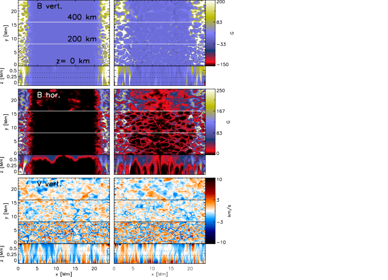
Figure 1: Magnetic field and vertical velocity close to the beginning ($t=1.5$ min, panels on the left) and end ($t=45$ min, panels on the right) of the simulation. Sub-panels in top panel from top to bottom show x-y slices of the vertical magnetic field strength at 3 different heights (400, 200 and 0 km) and a x-z slice of the simulation domain. $z=0$ km is defined as where the average temperature (over the entire simulation domain) at $t=0$ is $\approx$ 6000 K. The dashed lines in the bottom sub-panel mark the heights of the x-y slices. Initial distribution of field corresponds to unipolar (positive polarity) field at the left and right boundaries of the computational domain with field-free area between them. The two panels below show the same for the horizontal field and the vertical velocity, respectively.

The magnetic field is transported to the initially nearly field-free regions of the photosphere by two mechanisms, namely by horizontal diffusion (random walk) from the initial strip and by a process where the downflows due to the convective overshoot pull the field down from the canopy. With the simulation resolution, $\simeq$41 km in the horizontal direction, we do not achieve magnetic Reynolds numbers high enough to have local dynamo action. Therefore, we can exclude it as a source for the field in the initially nearly field-free regions. This does not exclude stretching and inductive amplification of the unsigned flux as a source in the later stages of the simulation. As we will later show when discussing the time evolution of the magnetic field topology this is an important process in supplying field to photospheric regions outside the initial strip. The prevalence of the spatial azimuth asymmetry throughout the simulation, both in height and time, points to a strong connection with the canopy which has the same asymmetry. This connection is also seen in the time evolution of the magnetic field (Fig. 2). In the initially field-free regions, the magnetic field appears at a given height nearly simultaneously at all locations in the horizontal plane. The fine structure of the field has a spatial scale of about 1 Mm, corresponding to the granulation scale. The field fills the volume starting from the top of the domain and reaches the surface after $\approx 10$ minutes, i.e, after a few granulation timescales. The horizontal diffusion of the field from the initial strip is seen as the slight increase with time of the width of the strong field region at $x\approx 0$ and $x\approx 24$. Its effect in filling the volume with field at distances greater than a couple of Mm from the strip is negligible compared to the flux transported down from the canopy. The nature of the downflows and canopy-like magnetic fields will be discussed in Section  4.

The dominance of downflows over horizontal diffusion in providing flux close to the surface is also seen in histograms of the magnetic field strength outside the initial strip taken at different times during the simulation (two first panels in Fig. 3). They show the strengthening of the horizontal and vertical fields. The vertical field is not unipolar as one would expect if the main transportation mechanism was horizontal diffusion. In fact, the signed vertical flux is significantly smaller than the unsigned flux at all times (right panel in Fig. 3). There are indications of saturation of the downflow mechanism after $\approx$ 600 seconds when the signed flux increase becomes faster than the increase of the unsigned flux.

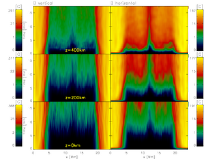
Figure 2: Time evolution of the mean (averaged along y-direction) vertical (left) and horizontal (right) magnetic field at z=400, 200 and 0 km during the first 18 minutes of the simulation.

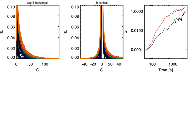
Figure 3: Histograms of the horizontal (left) and vertical (middle) magnetic fields at $z=220$ km for each time step of the simulation (blacks correspond to the beginning and reds to the end of the simulation) in a strip at $x=4-10$ Mm of the simulation domain (i.e., outside the initial strip of magnetic field). Right plot shows the time evolution of the signed (in black) and unsigned (in red) vertical magnetic flux in the strip.

To quantify the apparent speed at which the horizontal magnetic field is advected down from the canopy we look at when the average (in y-direction) total field strength at a given height becomes larger than 1 G or the unsigned vertical field exceeds 0.33 G or the horizontal field 0.66 G (Fig. 4). The limit was chosen based on images similar to Fig. 2 where 1 G outlines well the downward moving canopy. The thus computed average downward speed of the canopy’s base is found to be $\approx$1 km s^-1. The simulation domain extends $\approx$ 700 km above $\log(\tau)\approx 0$ in height so an average speed of 1 km s^-1 is consistent with field from the canopy reaching the solar surface in $\approx$ 10 minutes.

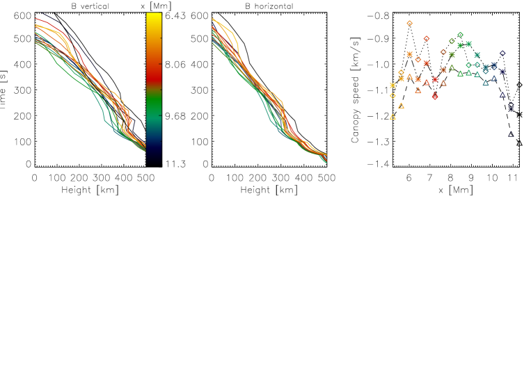
Figure 4: Transport of magnetic fields by downflows. Left and middle panels show the time when the base of the canopy (vertical and horizontal components) reaches a given height. The canopy base is considered to have reached a height when at that height the average (over a 400 km wide strip) vertical field strength is above 0.33 G or the horizontal field exceeds 0.66 G. The different colors are for different positions along the x-axis (shown in the color bar). The right panel shows the average downward velocity of the canopy base as a function of position along the $x$-axis. The velocity is derived from a linear fit between z=$0$ and $500$ km to the curves in the two other panels. Dotted line is for horizontal, dashed for vertical and dash-dotted for total field.

If the magnetic field is dragged down by downflows one would expect a prevalence of U-loops in the field reaching the surface, especially in the beginning of the simulation before the field topology becomes more complex as convection moves the dragged-down field in different directions. A 3-dimensional rendering of the magnetic field confirms this as is shown in Fig. 5. Color coding of the field lines represents vertical velocity (with red signifying downflows). It shows clearly that the U-loop is associated with a downflow.

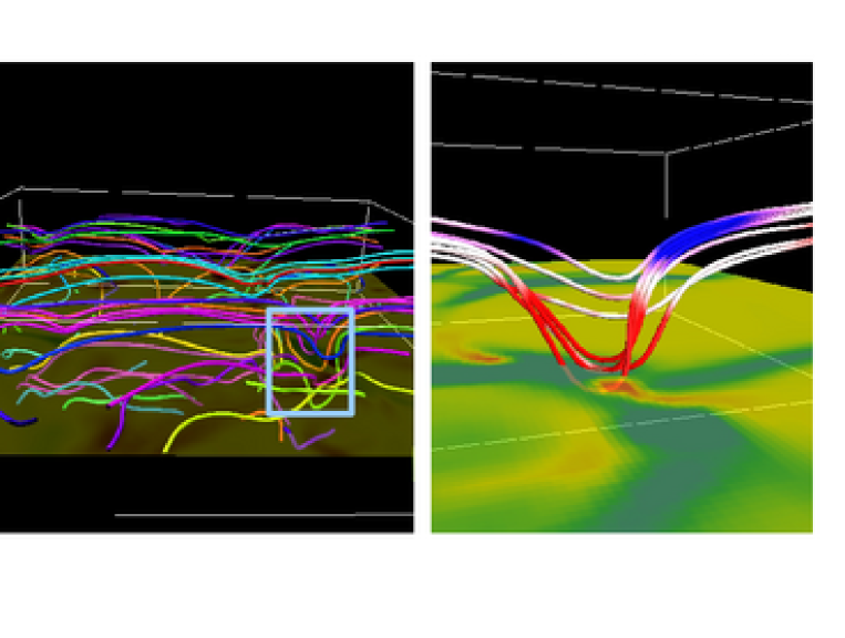
Figure 5: Left: Volume rendering of magnetic field lines in a subvolume of the simulation domain ($x=6-10$ Mm, $y=2-6$ Mm and $z=-0.5-0.7$ Mm). The snapshot is at $t=14.7$ min. Right: zoom into the region outlined by the light blue box. The surface is the ${\rm B_{x}}$ component of the magnetic field at $z=0$ km. Color of the field lines in the right panel shows the vertical velocity (red is a downflow, blue an upflow. Color scale saturates at $\pm$1 km s^-1). The volume rendering was made using the Visualization and Analysis Platform for Ocean, Atmosphere, and Solar Researchers (VAPOR, www.vapor.ucar.edu)

Since we are interested in the interaction of the canopy and the convective motions, we also performed an analysis to characterize the flux in the lower to mid photospheric layers as belonging to U-loops, $\Omega$-loops, or field lines going from below the surface to above the higher photospheric layers. For this purpose we define lower and upper surfaces at $z=-294$ and $z=406$ km. For each grid point $(x,y,z)$ within this domain the field through the point is traced in both directions until it leaves the subdomain. We label all the points along the field line as U-type if both ends of the field line exit the subdomain through the upper plane; the points are labeled as $\Omega$-type if both ends of the field line exit through the bottom plane; the field lines whose one end of which passes through the bottom plane and other end through the top plane are defined as being either positive or negative polarity depending on the orientation of the field.

The resulting classification of the magnetic field at z=$224$ km is shown for four timesteps in Fig. 6. The first snapshot is at 4.2 minutes, i.e., when the downflowing canopy reaches this height for the first time. At this time the downflows have had sufficient time to pull parts of the horizontal canopy down into the lower photosphere. The INW flux is located in the junctions of the intergranular lanes and it is nearly entirely in the form of U-loops or positive polarity field passing through the domain. The positive polarity field is due to flux expulsion: as 4.2 minutes is comparable to the lifetime of the granulation there has been enough time for flux expulsion to concentrate the very weak field in the region from $x=5$ to $20$ Mm into a number of isolated elements which thread the subdomain from bottom to top (and hence appear black in the topology maps). At later times, 14.1, 27.3 min, and 45 min, there are still U-loops present in the INW, but also a large amount of $\Omega$-loops are seen as well as positive polarity field. The U-loops appear as small bipoles in the bottom sub-panels showing the vertical field, with a vertical magnetic field strength which is generally stronger than in the $\Omega$-loops and in the vertical INW field. Because we do not have a supergranular scale flow in the simulation, flux which was originally in the unipolar network features begins to get concentrated into granular downflow lanes while at the same time gradually diffusing outward from its original location, as can be seen in the snapshot from 45 minutes.

Figure 7 displays the time evolution of the average unsigned flux density in the loops and single polarity field. Throughout the simulation most of the increase in unsigned flux in the volume within the height range $-294$ km $\leq z\leq 406$ km is from field lines which enter the volume from $z=-294$ km and leave through $z=406$ km. In between these two heights the unsigned field lines may be rather tangled and form small loops which contribute to the net unsigned flux. Since the field lines do not again leave the subdomain through the bottom they are not classified as loops. Unsigned flux of this type can increase through interaction with the near-surface turbulent eddies, and represents the pulling of the lowest lying flux above the surface into the convection zone. Higher lying flux is then pulled down, forming U-loops both ends of which pass through the plane $z=406$ km. During the first 10 minutes of the simulation U-loops dominate over $\Omega$-loops. They remain an important factor also in the later stages of the simulation. As the field in the originally non-magnetic region builds up, field lines with different topologies can interact and reconnect. The reconnection occurs preferentially in the higher levels where the lower pressures allow the flux tubes to expand horizontally and, therefore, more easily come into contact with other flux tubes. For this reason the reconnection tends to decrease the depth to which U-loops penetrate. Furthermore, magnetic tension can more easily pull the shallow, reconnected, U-loops out of the simulation domain. This may explain the decrease of flux associated with U-loops in Figure 7. Small-scale inductive stretching of the INW field lines over several turn-over times of the granulation can pull the now tangled field lines below the $z=-294$ km plane explaining the appearance of the $\Omega$-loops (green in Figs. 6 and  7). The average unsigned flux densities shown in Figure 7 are expected to depend strongly on the amount of signed flux in the network lane. The values are also likely affected by the choice of a potential field boundary condition and the height at which this boundary is placed. Furthermore, the amount of tangling within the photosphere in the simulations depends on the magnetic Reynolds number, with small-scale dynamo action occurring for sufficiently high values (Vögler & Schüssler, 2007; Pietarila Graham et al., 2010). For these reasons, while it is qualitatively clear that the canopy can supply a significant amount of flux to the photosphere, it is difficult to estimate the amount quantitatively from the present simulations.

Figure 6: Snapshots from the simulation at a height of 224 km at times t=4.2 (upper left), 14.1 (upper right), 27.3 (lower left), and 45 minutes (lower right). For each time the upper part of the panel shows the vertical component of the velocity saturated at $-2$ km s^-1 (blue) and $2$ km s^-1 (red). The middle parts are maps of the distribution of the different types of loops. U-type loops (field lines both ends of which leave through the top of the subdomain $-294$ km $\leq z\leq 406$ km are shown in red), $\Omega$-loops (both ends of which leave through the bottom of the subdomain) in green, field lines passing from the bottom to the top of the subdomain in black, and in the opposite direction in grey. The types of loops are only shown where the field exceeds $1$ G, all other regions are colored white. The bottom third of each snapshot shows the vertical component of the magnetic field, saturated at $\pm$ 50 G.

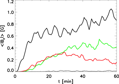
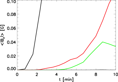
Figure 7: The time evolution of the different types of spatially averaged flux densities at height 224 km. The classification into U, $\Omega$ or straight-through topology is based on the subdomain $-294\leq z\leq 406$ km. The amount of unsigned flux associated with U-type loops is shown in red, $\Omega$-loops in green, field lines passing from the bottom to the top of the subdomain in black, and in the opposite direction in grey. The total amount of signed flux passing through the box has been subtracted from the black curve, so that the curve gives the increase in unsigned flux due to turbulent stretching and tangling of the field within the subdomain. The right panel shows a zoom into the lower left corner of the left panel.

Figure  8 shows the time evolution of the horizontal and vertical magnetic fields and the vertical velocity of the U-loops shown in Fig. 5. In the beginning there is only a little magnetic field in the junction of the intergranular lanes, but as the downflow plume reaches this height the field becomes stronger. The area with magnetic field becomes larger with time, consistent with the U-loop becoming more submerged. The U-loop is stretched and distorted as the field is further dragged into the downflow lanes. This is clearly seen in the fanning out of the horizontal field along the downflow lanes. After some time as the granulation evolves the field occupies a large fraction of the downflow lanes and is no longer as strong or as localized. The horizontal field strength in the feature is over 80 G at its strongest. The vertical field strengths are slightly lower, around 60 G. The size of the feature before it is spread out and weakened is less than an arcsecond across. This is a typical example of a submerging U-loop.

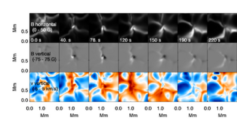
Figure 8: Time evolution of magnetic field and velocity at $z=220$ km in a region with magnetic flux appearing in the form of a U-loop from above. Top row: Horizontal magnetic field strength, middle row: vertical magnetic field strength, bottom row: vertical velocity (red corresponds to downflows and blue to upflows). Times for snapshots are given in the bottom of the top row images. The region is centered at $x=13.5$ Mm and $y=3.7$ Mm.

4 Discussion

In this paper we have looked at a scenario for transporting magnetic flux to the quiet Sun INW surface: already existing magnetic field is dragged down from a canopy-like configuration (consisting of mostly horizontal magnetic field) by downflows related to convective overshoot. An observational signature of the mechanism would be patches of linear polarization entirely embedded in downflows. Such patches were found to be common (8% of all linear polarization patches identified in the study) in the quiet-Sun INW by Danilovic et al. (2010a).

A similar process has been reported by Abbett (2007, in particular Fig.10 and the text describing it). The current study focuses on the canopy fields from network elements whereas Abbett studied convective dynamo action in the presence of an initially uniform field. While the rates and importance of the processes will differ in the two cases, the occurrence of the process in the two simulations suggests that it is robust. Importantly we note that Abbett (2007) simulations extended to coronal heights with a simpler treatment of the radiative losses. It should also be noted that the proposed mechanism is closely related to that of downward pumping as described by Thomas et al. (2002); Brummell et al. (2008), however, now applied to the INW surrounded by network magnetic field and overlaid by a canopy.

In the simulation nearly all of the horizontal field is in a high plasma-$\beta$ regime. If the field was stronger, it would appear more rigid to the downflows and, thus, would also less likely be dragged down. The horizontal field near the top of the simulation domain (our canopy) should be thought of as weaker flux lying beneath the actual chromospheric canopy as inferred from observations. This weaker canopy is there because the chromospheric canopy’s lower boundary is not sharp but is rather disturbed by shocks, overshooting convection, propagating waves and turbulence.

Several aspects of our simulation are idealized, especially the potential field boundary condition imposed at a relatively low height. The mechanism we have investigated, however, is likely to take place in the real Sun as well if there is field associated with the overlying canopy at heights reached by the overshooting convection. The field dragged down below the surface by the downward plumes could then act as an additional source for the generation of more field.

Danilovic et al. (2010a) present statistics of linear polarization patches in an INW region observed with the IMaX instrument on Sunrise. They find that 8% of the observed linear polarization patches are associated purely with signatures of submergence. Moreover, 16% of all the observed patches begin in a downflow. These features are not consistent with emergence of flux from below, where an upflow would initially be expected. However, they are compatible with the scenario proposed here. Furthermore, the sizes and field strengths of the observed linear polarization patches are comparable with the features seen in the simulation. Of course, we cannot rule out other possible explanations for the linear polarization features embedded in downflows.For example, the local dynamo simulations suggest the existence of very small-scale loops with footpoints embedded in intergranular lanes (Vögler & Schüssler, 2007; Schüssler & Vögler, 2008). Their polarimetric signature can vary as they are redistributed by the turbulent flows (Danilovic et al., 2010a). In addition, $\Omega$-loops, emerged or generated by reconnection above the solar surface, can be pulled back down by convective motions (Chae et al., 2004; Stein & Nordlund, 2006) producing the linear polarization features associated with downflows as a result.

It is difficult for a number of reasons to conclusively identify the mechanism proposed here in observations of the real Sun. We expect a mixture of processes to transport magnetic field to the INW and only a small portion of the observed linear polarization patches are embedded in downflows. In the simulation the cleanest examples are seen in the beginning when there is only little flux outside the initial strip. As the simulation evolves, the magnetic field configuration becomes more complex. One possible observational test would be to look for spatial patterns in the azimuth of INW linear polarization patches embedded in downflows. This would, however, require solving the 180 degree ambiguity correctly.

References

- Abbett (2007) Abbett, W. P. 2007, ApJ, 665, 1469
- Barthol et al. (2011) Barthol, P., Gandorfer, A., Solanki, S. K., & et al. 2011, Sol. Phys., 268, 1
- Berkefeld et al. (2011) Berkefeld, T., Schmidt, W., Soltau, D., et al. 2011, Sol. Phys., 268, 103
- Brummell et al. (2008) Brummell, N. H., Tobias, S. M., Thomas, J. H., & Weiss, N. O. 2008, ApJ, 686, 1454
- Centeno et al. (2007) Centeno, R., Socas-Navarro, H., & Lites, B. 2007, ApJ, 666, L137
- Chae et al. (2004) Chae, J., Moon, Y. J., & Pevtsov, A. A. 2004, ApJ, 602, L65
- Danilovic et al. (2010a) Danilovic, S., Beeck, B., Pietarila, A., et al. 2010a, ApJ, 723, L149
- Danilovic et al. (2010a) Danilovic, S., Schüssler, M., & Solanki, S. K. 2010b, A&A, 513, A76
- de Wijn et al. (2009) de Wijn, A. G., McIntosh, S. W., & De Pontieu, B. 2009, ApJ, 702, L168
- Gabriel (1976) Gabriel, A. H. 1976, Royal Society of London Philosophical Transactions Series A, 281, 339
- Gandorfer et al. (2011) Gandorfer, A., Grauf, B., Barthol, P., et al. 2010, Sol. Phys., 268, 35
- Hagenaar et al. (2003) Hagenaar, H. J., Schrijver, C. J., & Title, A. M. 2003, ApJ, 584, 1107
- Kosugi et al. (2007) Kosugi, T., Matsuzaki, K., Sakao, T., & et al. 2007, Sol. Phys., 243, 3
- Lites et al. (2001) Lites, B. W., Elmore, D. F., & Streander, K. V. 2001, in Astronomical Society of the Pacific Conference Series, Vol. 236, Advanced Solar Polarimetry – Theory, Observation, and Instrumentation, ed. M. Sigwarth, 33
- Martínez González & Bellot Rubio (2009) Martínez González, M. J. & Bellot Rubio, L. R. 2009, ApJ, 700, 1391
- Martínez González et al. (2007) Martínez González, M. J., Collados, M., Ruiz Cobo, B., & Solanki, S. K. 2007, A&A, 469, L39
- Martínez Pillet et al. (2011) Martínez Pillet, V., del Toro Iniesta, J. C., Álvarez-Herrero, A., & et al. 2011, Sol. Phys., 268, 57
- Petrovay & Szakaly (1993) Petrovay, K. & Szakaly, G. 1993, A&A, 274, 543
- Pietarila et al. (2010) Pietarila, A., Cameron, R., & Solanki, S. K. 2010, A&A, 518, A50
- Pietarila Graham et al. (2010) Pietarila Graham, J., Cameron, R., & Schüssler, M. 2010, ApJ, 714, 1606
- Ploner et al. (2001) Ploner, S. R. O., Schüssler, M., Solanki, S. K., & Gadun, A. S. 2001, in Astronomical Society of the Pacific Conference Series, Vol. 236, Advanced Solar Polarimetry – Theory, Observation, and Instrumentation, ed. M. Sigwarth, 363
- Schüssler & Vögler (2008) Schüssler, M. & Vögler, A. 2008, A&A, 481, L5
- Shimizu et al. (2008) Shimizu, T., Nagata, S., Tsuneta, S., et al. 2008, Sol. Phys., 249, 221
- Solanki et al. (2010) Solanki, S. K., Barthol, P., Danilovic, S., et al. 2010, ApJ, 723, L127
- Stein & Nordlund (2006) Stein, R. F. & Nordlund, Å. 2006, ApJ, 642, 1246
- Suematsu et al. (2008) Suematsu, Y., Tsuneta, S., Ichimoto, K., et al. 2008, Sol. Phys., 249, 197
- Thomas et al. (2002) Thomas, J. H., Weiss, N. O., Tobias, S. M., & Brummell, N. H. 2002, Nature, 420, 390
- Trujillo Bueno et al. (2004) Trujillo Bueno, J., Shchukina, N., & Asensio Ramos, A. 2004, Nature, 430, 326
- Tsuneta et al. (2008) Tsuneta, S., Ichimoto, K., Katsukawa, Y., et al. 2008, Sol. Phys., 249, 167
- Vögler & Schüssler (2007) Vögler, A. & Schüssler, M. 2007, A&A, 465, L43
- Vögler et al. (2005) Vögler, A., Shelyag, S., Schüssler, M., et al. 2005, A&A, 429, 335
- Wedemeyer-Böhm et al. (2009) Wedemeyer-Böhm, S., Lagg, A., & Nordlund, Å. 2009, Space Science Reviews, 144, 317