Quantum frequency estimation with trapped ions and atoms

Abstract

We discuss strategies for quantum enhanced estimation of atomic transition frequencies with ions stored in Paul traps or neutral atoms trapped in optical lattices. We show that only marginal quantum improvements can be achieved using standard Ramsey interferometry in the presence of collective dephasing, which is the major source of noise in relevant experimental setups. We therefore analyze methods based on decoherence free subspaces and prove that quantum enhancement can readily be achieved even in the case of significantly imperfect state preparation and faulty detections.

The ultra-precise estimation of physical parameters is of great importance for countless applications, such as atomic clocks, gravitational wave detectors, laser gyroscopes or microscopy. Quantum enhanced precision measurements have the potential to significantly increase the precision of parameter estimation compared to classical methods in such applications Giovannetti et al. (2004). This is generally achieved by preparing a quantum probe-state which has a higher sensitivity with respect to the quantity to be estimated. Assuming that this probe consists of $N$ non-interacting, identical subsystems (e.g. $N$ particles), the estimation uncertainty in many applications including optical or atomic interferometry can then ideally be improved from the standard quantum limit (SQL), which scales like $1/\sqrt{N}$, to the Heisenberg limit, which scales like $1/N$ Giovannetti et al. (2006); Boixo et al. (2007). Endeavors to attain the Heisenberg limit (or at least to beat the SQL) are made in many branches of physics including quantum photonics Dowling (2008) and atomic physics Leibfried et al. (2004); Meyer et al. (2001); Leroux et al. (2010); Louchet-Chauvet et al. (2010); Gross et al. (2010); Riedel et al. (2010). In atomic physics, the measurement of atomic transition frequencies with Ramsey interferometry has been established as an important tool, not only for general spectroscopic purposes but also to determine frequency standards on which atomic clocks are based on Diddams et al. (2004). Improvements of Ramsey interferometry via quantum effects are therefore highly desirable. As in other quantum technologies like quantum computing and communication, the biggest obstacle for the realization of such a quantum interferometer is the presence of unavoidable noise and imperfections. A practical quantum sensor must therefore use probe-states which are robust under realistic circumstances, as well as preparation and detection schemes which can be performed with high fidelity.

In this paper we analyze methods for quantum enhanced estimation of atomic transition frequencies with Ramsey interferometry, and generalizations thereof, which can improve the measurement uncertainty to the Heisenberg limit in the presence of noise, and which tolerate imperfect state preparation and detection. A scheme for quantum enhanced Ramsey interferometry has been proposed some time ago Bollinger et al. (1996), but it has subsequently been shown that in the presence of noise, in form of uncorrelated dephasing, the scheme has only little or no advantage compared to its classical counterpart Huelga et al. (1997). However, recent experimental breakthroughs with closely spaced particles, particularly ions stored in linear Paul traps Monz et al. (2011); Roos et al. (2006); Langer et al. (2005); Kielpinski et al. (2001), show that the major source of noise in these systems consists of correlated dephasing. Motivated by this insight we first analyze conventional Ramsey interferometry and show that in the presence of correlated dephasing hardly any quantum enhancement can be achieved. We therefore discuss alternative methods which make use of decoherence free subspaces Lidar and Whaley (2003) and show that they lead to quantum enhanced precision even in the presence of significantly imperfect state preparation and faulty detections. Our approach is mainly motivated by recent experiments with trapped ions, but it can also be applied to cold atoms stored in optical lattices Jaksch and Zoller (2005). The main body of this paper concisely summarizes our results. Details of calculations can be found in the appendices.

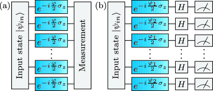
Figure 1: (a) Schematic Ramsey interferometer. (b) Generalized setup where atoms acquire different phases (see text).

We consider $N$ two-level atoms or ions, with internal states $|0\rangle$ and $|1\rangle$, which are, e.g., stored in a linear Paul trap. These atoms are prepared in an input state $|\psi_{in}\rangle$ and undergo the process shown in Fig. 1(a), i.e. each atom accumulates a phase $\varphi$ during a time $t$ and is finally measured. The process is repeated $\nu$ times and based on the measurement outcomes the phase can be estimated. For simplicity we assume that the measurement and preparation times are much smaller than $t$, such that the total time of the experiment is given by $T=\nu t$. It is our goal to make the uncertainty of the estimated phase as small as possible for a given $T$ and $N$.

In conventional Ramsey interferometry the input state is given by the product state $|\psi_{in}^{pro}\rangle=[(|0\rangle+|1\rangle)/\sqrt{2}]^{\otimes N}$ which is prepared by a $\pi/2$-pulse using a laser with frequency $\omega_{L}$ which is slightly detuned from the atomic transition frequency $\omega$. Note that for simplicity in this paper we identify $\pi/2$-pulses with Hadamard gates which has no effect on the estimation uncertainty. Each atom then undergoes a free evolution of duration $t$ before a second $\pi/2$-pulse (using the same laser) and a measurement of the atomic state is performed. During the time $t$ the atoms gather up a relative phase $\varphi=(\omega-\omega_{L})t$ which can be estimated from the measurement data. If $\omega_{L}$ and $t$ are known, we therefore obtain an estimate $\omega_{est}$ of the frequency $\omega$ with an uncertainty given by Braunstein and Caves (1994); Braunstein et al. (1996)

$$\Delta\omega=\left\langle\left(\frac{\omega_{est}}{|\partial\langle\omega_{est}\rangle/\partial\omega|}-\omega\right)^{2}\right\rangle^{1/2}$$ (1)

which, for unbiased estimators, is simply the standard deviation. The uncertainty, or precision, $\Delta\omega$ is bounded from below by the (quantum) Cramér-Rao bound Helstrom (1976); Braunstein and Caves (1994); Braunstein et al. (1996)

$$\Delta\omega\geq\frac{1}{\sqrt{\nu F}}\geq\frac{1}{\sqrt{\nu F_{Q}}}=\frac{1}{\sqrt{TF_{Q}/t}}\equiv\Delta\omega_{min},$$ (2)

where $F$ is the Fisher information and $F_{Q}$ is the quantum Fisher information (QFI). Expressions for $F$ and $F_{Q}$ can be found in Braunstein et al. (1996); Demkowicz-Dobrzanski et al. (2009) and Appendices B, C. The Fisher information depends on the state of the system before the measurement and the measurement itself while the QFI depends only on the state before the measurement. The first bound in Eq. (2) can be reached via maximum likelihood estimation for large $\nu$ (or $T$) and the second bound by an optimal measurement which always exists Braunstein and Caves (1994).

If we assume that our pure input state remains pure, a product state $|\psi_{in}^{pro}\rangle$ as input then leads to the SQL precision $\Delta\omega_{min}=1/\sqrt{TtN}$, whereas an entangled ($N$-particle) Greenberger-Horne-Zeilinger (GHZ) state, $|\psi_{in}^{GHZ}\rangle=(|0\rangle^{\otimes N}+|1\rangle^{\otimes N})/\sqrt{2}$, improves the precision to $\Delta\omega_{min}=1/\sqrt{Tt}N$, i.e. the Heisenberg limit Bollinger et al. (1996). However, under realistic conditions, the pure input state will degrade into a mixture due to unavoidable noise. For the systems considered here the dominant source of noise is dephasing caused by fluctuating (stray) fields leading to random energy shifts of the atomic levels. As shown in Huelga et al. (1997); Shaji and Caves (2007), the advantage of a GHZ state deteriorates in case of uncorrelated dephasing, leading to exactly the same optimal precision as a product state which has merely SQL scaling. However, this is not the situation commonly encountered in ion traps or atoms in optical lattices where particles are very closely spaced. Here, the particles are subject to the same fluctuations which leads to correlated dephasing such that the time evolution of the system state $\rho$ is determined by

$$\dot{\rho}=-\mathrm{i}\frac{\delta}{2}[S_{z},\rho]+\frac{\gamma}{2}\left(L\rho L-\frac{1}{2}L^{2}\rho-\frac{1}{2}\rho L^{2}\right),$$ (3)

where $\delta=\omega-\omega_{L}$, $\gamma$ is a dephasing rate and $L=S_{z}\equiv\sum_{j=1}^{N}\sigma_{z}^{j}$, where $\sigma_{z}^{j}$ is the Pauli $z$-operator acting on atom $j$. The fact that Eq. (3) describes the dominant source of noise in the setups considered in this paper was very clearly shown in a number of recent experiments Monz et al. (2011); Roos et al. (2006); Langer et al. (2005); Kielpinski et al. (2001). Equation (3) can be derived via a Langevin-equation approach by assuming that the atoms are subject to level shifts caused by the same fluctuating field with a sharp time correlation function (see Appendix A for details). This is typically the case in experiments, e.g. in the ion trap experiment Monz et al. (2011), where the dominant source of noise is caused by fluctuations of the homogeneous magnetic field which is required to lift Zeeman degeneracies and which affects all ions in an equal manner.

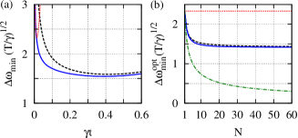
Figure 2: (Color online) (a) Precision $\Delta\omega_{min}$ versus duration of the free evolution for $N=6$ atoms. The minima of the curves define $\Delta\omega_{min}^{opt}$. (b) Best possible precision $\Delta\omega_{min}^{opt}$ versus atom number $N$. In both figures the dotted (red) line corresponds to a GHZ state, the dashed (black) line to a product state and the solid (blue) line to the optimal precision. In (b) we also show the precision corresponding to a product/GHZ state undergoing uncorrelated dephasing (dashed-dotted, green line).

Suppose we consider states which are symmetric under particle exchange, then we can use a Fock representation in which $S_{z}=n_{0}-n_{1}$, where $n_{i}\equiv a_{i}^{\dagger}a_{i}$, and $a_{i}^{\dagger}$ ($a_{i}$) are bosonic creation (annihilation) operators of an atom in state $|i\rangle,\,i=0,1$. We can then rewrite Eq. (3) to obtain

$$\dot{\rho}=-\mathrm{i}\delta[n_{0},\rho]+2\gamma\left[n_{0}\rho n_{0}-\frac{1}{2}n_{0}^{2}\rho-\frac{1}{2}\rho n_{0}^{2}\right],$$ (4)

and a symmetric, pure input-state has the form $|\psi_{in}\rangle=\sum_{k=0}^{N}\alpha_{k}|k,N-k\rangle$, where $|k,N-k\rangle$ is a Fock state with $k$ ($N-k$) atoms in state $|0\rangle$ ($|1\rangle$). Equation (4) can be solved analytically [see Eq. (43)] which yields the system state immediately before the measurement which can be used to calculate the QFI. A GHZ state is in this representation formally equivalent to a NOON-state known from optical interferometry Dowling (2008), $|\psi_{in}\rangle=(|N,0\rangle+|0,N\rangle)/\sqrt{2}$. Using this state as initial state leads, via the QFI, to the precision

$$\Delta\omega_{min}=\frac{1}{\sqrt{Tt}N\mathrm{e}^{-\gamma N^{2}t}}\geq\sqrt{\frac{2\mathrm{e}\gamma}{T}}\equiv\Delta\omega_{min}^{opt}.$$ (5)

The quantity $\Delta\omega_{min}^{opt}$ is found by using an optimal time $t_{opt}=1/2\gamma N^{2}$ for each experimental run. As can be seen, $\Delta\omega_{min}^{opt}$ has no dependency on $N$ and therefore there is no advantage using a GHZ state in the presence of collective dephasing. The precision $\Delta\omega_{min}$ and $\Delta\omega_{min}^{opt}$ corresponding to a product state can be calculated numerically leading to $\Delta\omega_{min}^{opt}\approx(\sqrt{2}+0.87/N^{0.90})\sqrt{\gamma/T}$ which has no SQL scaling and does not even approach zero for large $N$, but is still better than the GHZ case (see Fig. 2).

A decisive feature of collective dephasing is the existence of decoherence free subspaces (DFSs) Lidar and Whaley (2003) which are given by states such that $L|\psi_{DFS}\rangle=0$. However, since $L=S_{z}$ in Eq. (3) a highly robust DFS state would be stationary and hence useless for frequency estimation. Ideally, one would therefore use input states which lead to an optimal trade-off between gain in precision and robustness which can be found by maximizing the QFI with respect to all possible input states. In Appendix B we show that the maximal QFI can be attained by states which are symmetric under particle exchange leading to a considerable simplification of the optimization problem. Results are shown in Fig. 2. As can be seen the best possible state leads only to a marginal improvement over a product state. For comparison, in Fig. 2(b) we also plot the precision corresponding to $|\psi_{in}^{pro}\rangle$ which is subject to uncorrelated dephasing Huelga et al. (1997). Evidently, correlated dephasing is significantly more destructive than uncorrelated dephasing.

To make use of the coherence preserving features of DFSs we have to alter the dynamics of the system such that the incoherent part of Eq. (3) is zero and the coherent part is non-zero. To this end we consider a scheme consisting of $N$ atoms ($N$ even), where half of the atoms accumulate a phase $\varphi_{1}$ and the other half $\varphi_{2}$. Such a scheme is realized in a system where, e.g., every odd atom has a transition frequency $\omega_{1}$ and every even atom has a transition frequency $\omega_{2}$ [see Fig. 1(b)] and our goal is to estimate the frequency difference $\delta\equiv\omega_{1}-\omega_{2}$ (see Appendix A.2). If fluctuating fields lead to the same energy shift in both transitions the incoherent part of the master equation (3) vanishes if a DFS state of the form $|\psi_{in}\rangle=(|0101\ldots 01\rangle+|1010\ldots 10\rangle)/\sqrt{2}$ is used. Via the QFI, we then obtain the bound for the precision $\Delta\delta_{min}=2/\sqrt{Tt}N$ which has Heisenberg scaling even in the presence of correlated dephasing. We should note here that in general we can use arbitrary orderings of the atoms in Fig. 1(b). The input state then takes the form

$$|\psi_{in}\rangle=\frac{1}{\sqrt{2}}(|i_{1},i_{2},\ldots,i_{N}\rangle+\prod_{j=1}^{N}\sigma_{x}^{j}|i_{1},i_{2},\ldots,i_{N}\rangle),$$ (6)

where $i_{j}=0,1$ and $\sum_{j=0}^{N}i_{j}=N/2$ (i.e. $i_{j}=0$ occurs as many times as $i_{j}=1$) and atoms with $i_{j}=0$ ($i_{j}=1$) accumulate the phase $\varphi_{1}$ ($\varphi_{2}$). The described dynamics can be obtained, e.g., by choosing the two transitions to be within the same Zeeman manifold such that the difference of the magnetic quantum numbers of each transition is equal, and thus a (weak) fluctuating magnetic field leads to the same energy shifts. This was demonstrated in a recent experiment with two ions in a linear Paul trap revealing a significant increase in the coherence time Roos et al. (2006). The same ideas were furthered by an experimental study of non-perfect input states Chwalla et al. (2007). In both experiments, an additional electric quadrupole field was used to obtain $\omega_{1}\neq\omega_{2}$ and from the measured frequency difference the electric quadrupole moment was determined.

The above experiments also offers an alternative view of the fact that Heisenberg scaling can be obtained in this setup. In Ref. Roos et al. (2006) a ‘designer atom’ was constructed consisting of two physical atoms with two internal, logical states $|0\rangle_{L}\equiv|01\rangle$ and $|1\rangle_{L}\equiv|10\rangle$ which are decoherence free. A state of the form $(|0101\ldots 01\rangle+|1010\ldots 10\rangle)/\sqrt{2}$ is then equivalent to a decoherence free GHZ state of $n=N/2$ designer atoms, $|\psi_{in}\rangle_{L}=(|00\ldots 0\rangle_{L}+|11\ldots 1\rangle_{L})/\sqrt{2}$. The states $|0\rangle_{L},\,|1\rangle_{L}$ accumulate a relative phase $\delta t$, and so it is straightforward that $|\psi_{in}\rangle_{L}$ leads to a sensitivity $\Delta\delta_{min}=1/\sqrt{Tt}n$.

We can also conceive a situation where the fluctuating field shifts the transition frequency $\omega_{1}$ of half of the atoms and the transition frequency $\omega_{2}$ of the other half by the same magnitude but opposite sign. For the setup shown in Fig. 1(b), this means that we have to replace the noise operator in Eq. (3) by $L=\sum_{j=1}^{N}(-1)^{j}\sigma_{z}^{j}$ and a GHZ state would be decoherence free. We can utilize this for quantum enhanced precision measurements by performing a Ramsey-type experiment but now with up to two lasers of frequency $\omega_{L1}$ and $\omega_{L2}$ such that half of the atoms accumulate a relative phase $\varphi_{1}=(\omega_{1}-\omega_{L1})t\equiv\delta_{1}t$ and the other half $\varphi_{2}=(\omega_{2}-\omega_{L2})t\equiv\delta_{2}t$. The Hamiltonian can then be written as (see Appendix A.3)

$$H=\frac{1}{4}(\delta_{1}+\delta_{2})S_{z}+\frac{1}{4}(\delta_{2}-\delta_{1})L,$$ (7)

where the second term vanishes if applied to a GHZ state. If the laser frequencies are known, the quantity which can be estimated with this setup is therefore given by $\Omega\equiv(\omega_{1}+\omega_{2})/2$ and the corresponding precision, which can be calculated via the QFI, is given by $\Delta\Omega_{min}=1/\sqrt{Tt}N$ which has Heisenberg scaling. The above discussion can again be generalized to an arbitrary ordering of the atoms as long as we use a GHZ state as input. The setup can be realized, e.g., by using transitions $|m\rangle\leftrightarrow|\tilde{m}\rangle$ with frequency $\omega_{1}$ and $|-m\rangle\leftrightarrow|-\tilde{m}\rangle$ with frequency $\omega_{2}$, i.e. the two ground states (with magnetic quantum numbers $\pm m$) and the two excited states (with magnetic quantum numbers $\pm\tilde{m}$) are in the same Zeeman manifold, respectively, such that (fluctuating) magnetic fields cause first order Zeeman shifts of the same magnitude but opposite sign Roos (2005); Chwalla et al. (2007). Note that the quantity to be estimated, $\Omega$, is magnetic field independent (in first order), i.e. the situation is similar to a clock transition, and $\Omega$ might therefore serve as a frequency standard. Moreover, $\Omega$ can easily be chosen to be in the optical domain which is desirable for atomic clocks Diddams et al. (2004).

We also note that, similar to the case of estimating $\delta$, we can introduce decoherence free logical states $|0\rangle_{L}\equiv|00\rangle$ and $|1\rangle_{L}\equiv|11\rangle$ which accumulate a relative phase $2\Omega t$. A GHZ state of $N$ atoms is then simply a GHZ state of $n=N/2$ logical states and the precision is given by $\Delta\Omega_{min}=1/\sqrt{Tt}2n$, the factor of 2 arising from the factor of 2 in the relative phase of $|0\rangle_{L}$ and $|1\rangle_{L}$.

An optimal measurement for the two schemes discussed above, i.e. a measurement for which $F=F_{Q}$ [see Eq. (2)], is given by a $\pi/2$-pulse and a measurement of each atom in the $\{|0\rangle,|1\rangle\}$-basis [see Fig. 1(b)]. However, in practice there will be imperfections both in the preparation of the input state and the measurement. A faulty measurement of an atom can be modeled using the measurement operators

$$\Pi_{i}=\frac{1}{2}(1+\eta_{M})|i\rangle\langle i|+\frac{1}{2}(1-\eta_{M})\sigma_{x}|i\rangle\langle i|\sigma_{x},$$ (8)

where $i=0,1$, and $\eta_{M}$ is the likeliness that we get the correct measurement result. Also, we assume that the actual input state is of the form

$$\rho_{in}=\xi(N)|\psi_{in}\rangle\langle\psi_{in}|+\frac{1}{2^{N}}[1-\xi(N)]\openone,$$ (9)

i.e. we prepare the ideal input state $|\psi_{in}\rangle$ with fidelity

$$f=\langle\psi_{in}|\rho_{in}|\psi_{in}\rangle=\xi(N)+\frac{1}{2^{N}}[1-\xi(N)],$$ (10)

and hence $f\approx\xi(N)$ for $N\gg 1$. The error model (9) is a worst case scenario since the identity matrix does not yield any phase information. Analogously, we assume that a $\pi/2$-pulse is given by the operation

$$\eta_{H}\rho_{id}+\frac{1}{2}(1-\eta_{H})\openone,$$ (11)

i.e. $\eta_{H}$ characterizes the probability to perform a perfect $\pi/2$-pulse leading to an ideal state $\rho_{id}$ (see Appendix C). We can then calculate the Fisher information for both schemes and therefore the Cramér-Rao bounds,

$$\Delta\Omega_{min}=\frac{\Delta\delta_{min}}{2}=\frac{1}{\sqrt{Tt}N\xi(N)\eta_{H}^{N}\eta_{M}^{N}},$$ (12)

where we assumed that $\varphi_{1}\pm\varphi_{2}=\pi/N$ (‘+’ for $\Delta\Omega_{min}$; ‘-’ for $\Delta\delta_{min}$), which can always be achieved by a feedback setup which appropriately adjusts, e.g., the electric quadrupole field, laser frequencies or/and the evolution time $t$. We note that the state which was prepared in Chwalla et al. (2007) leads to the same result for $\xi(N)=1/2$ and $N=2$. The term $\xi(N)\eta_{H}^{N}\eta_{M}^{N}$ in Eq. (12) might, at first glance, lead to the conclusion that faulty state preparation and detection annihilates the advantage gained by using a DFS. To show that this is not the case we compare the precisions (12) to those obtained using conventional Ramsey spectroscopy with a product-state $|\psi_{in}^{pro}\rangle$ as input. In this case we would use $N/2$ atoms to estimate $\omega_{1}$ and the others to estimate $\omega_{2}$. For a fair comparison we assume uncorrelated dephasing which can in principle always be achieved by placing the atoms in different traps. Assuming that $|\psi_{in}^{pro}\rangle$ is created by $N$ $\pi/2$-pulses, the corresponding precision then reads $\Delta\omega_{1,min}=\Delta\omega_{2,min}=\sqrt{4\mathrm{e}\gamma/NT}/\eta_{H}^{2}\eta_{M}$, and the precisions of the quantities to be estimated is given by $\Delta\Omega_{min}=\frac{1}{2}\Delta\delta_{min}\approx\Delta\omega_{1,min}/\sqrt{2}$ which have to be compared to Eq. (12). In both cases this leads to the constraint

$$\xi(N)\geq\xi_{min}\equiv\frac{1}{\eta_{H}^{N-2}\eta_{M}^{N-1}\sqrt{2N\gamma t\mathrm{e}}},$$ (13)

i.e. whenever the above inequality is fulfilled the DFS schemes beat conventional Ramsey spectroscopy. An example is shown in Fig. 3(a). With current ion trap experiments gate and readout fidelities in excess of $\eta_{H}=0.98$ and $\eta_{M}=0.99$ have been achieved Burrell et al. (2010). Furthermore, we assumed that using a DFS scheme leads to a coherence time which is 3 times longer than the coherence time of a single atom. This is a rather conservative estimate which has already been exceeded in experiments Monz et al. (2011). As can be seen the bound for the state fidelity $\xi(N)$ is surprisingly low. In the experiment described in Monz et al. (2011) a 50.8% fidelity for a $N=14$ GHZ state was achieved. For our scheme it would be required to manipulate this GHZ state by transfering half of the atoms into a different internal state. Naturally this would be done by addressing, for example, the second $N/2$ neighbouring atoms by an appropriate sequence of laser pulses, i.e., crucially, it is not required to address atoms individually. This would of course decrease $\xi(N)$ but even if it reduces it to, say, 20% (which is a very conservative assumption) we still beat conventional Ramsey spectroscopy.

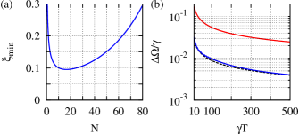
Figure 3: (Color online) (a) Minimum fidelity of the input state versus number of atoms $N$ [cf. Eq. (13)]. (b) Maximum likelihood estimation uncertainty $\Delta\Omega$ versus total measurement time $T$ for $N=20$ and $\xi(N)=0.6$. The lower, solid (blue) line corresponds to a GHZ state and the upper, solid (red) line to a product state. The dashed (black) line is given by Eq. (12). In both figures we set $\eta_{H}=0.98$, $\eta_{M}=0.99$, $\gamma t=3$.

The bounds (12) can be reached using maximum likelihood estimation in the limit of large $\nu$ (or $T$). In practice it is certainly highly relevant how large $\nu$ has to be such that the actual estimation uncertainty is close to the bound. Suppose we perform $\nu$ experimental runs and obtain the results $n_{1},\ldots,n_{\nu}$, where $n_{j}$ is the number of times the state $|0\rangle$ is measured in each run, and the total number of even $n_{j}$ is $\nu_{e}$. It turns out that the maximum likelihood estimators $\Omega_{est}$ and $\delta_{est}$ depend only on $\nu_{e}$ (see Appendix D). Using the probability distribution for $\nu_{e}$ and Eq. (1) we can then calculate, e.g. the estimation uncertainty $\Delta\Omega$ for finite $\nu$. A result is shown in Fig. 3(b) depending on the total time $T=\nu t$ of the experiment (lower solid line) for $\varphi_{1}+\varphi_{2}=\pi/N$. As can be seen the estimation uncertainty quickly approaches the lower bound (dashed line). We also show the estimation uncertainty and the lower bound for conventional Ramsey spectroscopy with $|\psi_{in}^{pro}\rangle$ (upper solid line; the two quantities are indistinguishable on the scale of the figure). Evidently, even for small $T$, the DFS scheme easily outperforms conventional Ramsey spectroscopy. We note that the corresponding plots for estimating $\delta$ would be identical to the ones shown but larger by a factor of two.

To conclude, we have shown that correlated dephasing significantly diminishes the precision of frequency estimation with standard Ramsey interferometry. On the other hand, it allows for the existence of DFSs which we used to construct and analyze generalized Ramsey setups which beat the SQL even in the presence of faulty detection and significantly imperfect state preparation. The proposed schemes for quantum enhanced frequency estimation are therefore feasible with current experimental technology and can lead to improved spectroscopic methods with a variety of important applications in metrology.

Appendix A Noise model

In this appendix we give a detailed description of the noise model and the derivation of Eq. (3). An alternative derivation is given by coupling the atoms to a bosonic bath, similar to the methods described in Palma et al. (1996); Carmichael (1999). However, the following derivation, which is based on a Langevin-equation approach, is physically more intuitive for the systems considered in this paper, i.e. atoms which are subject to fluctuating classical fields.

Consider $N$ two-level atoms (or ions) with internal states $\{|0\rangle_{j},\,|1\rangle_{j}\}$ and transition frequencies $\omega_{j}$ which are subject to a time-dependent, fluctuating field leading to random energy shifts of the transitions. The Hamiltonian can then be written as

$$H = \frac{1}{2}\sum_{j=1}^{N}\omega_{j}\sigma_{z}^{j}+B(t)\sum_{j=1}^{N}\varepsilon_{j}\sigma_{z}^{j}$$ (14)

$$\equiv H_{0}+B(t)L,$$

where (the real numbers) $B(t)$ and $\varepsilon_{j}$ characterize the field strength and how it affects atom $j$, and $\sigma_{z}^{j}=|0\rangle_{j}\langle 0|-|1\rangle_{j}\langle 1|$ is the Pauli $z$-operator acting on atom $j$. Writing $B(t)\equiv\sqrt{\gamma/2}\xi(t)$ the Schrödinger equation then takes the form

$$\frac{d}{dt}|\psi\rangle=-\mathrm{i}H_{0}|\psi\rangle-\mathrm{i}\sqrt{\frac{\gamma}{2}}L|\psi\rangle\xi(t).$$ (15)

The random fluctuations of the field are captured in $\xi(t)$ and Eq. (15) is therefore an example of a Langevin equation Gardiner (2004). Assuming that $\xi(t)$ has zero mean and very rapidly decaying time correlations, we can write

$$\overline{\xi(t)} = 0,$$ (16)

$$\overline{\xi(t)\xi(t^{\prime})} = \delta(t-t^{\prime}),$$ (17)

where the overbar denotes the mean value, i.e. we make the idealization that $\xi(t)$ is white noise. Equation (15) can then be written as a stochastic differential equation

$$|d\psi\rangle=-\mathrm{i}H_{0}|\psi\rangle dt-\mathrm{i}\sqrt{\frac{\gamma}{2}}L|\psi\rangle dW\qquad(S),$$ (18)

where $dW=\xi(t)dt$ is a Wiener increment Gardiner (2004). The $(S)$ indicates that we have to interpret this equation in the Stratonovich sense. The reason for this is given by the fact that Eq. (17) is an idealization. In reality this correlation function will have a finite width (but which is small compared to any other relevant time scale). In such a case the stochastic differential equation (18) has to be interpreted in the Stratonovich sense. A detailed discussion of this point can be found in Chapter 6.5 in Gardiner (2004). Transforming Eq. (18) into Ito form, using the standard rules Gardiner (2004), leads to

$$|d\psi\rangle=\left(-\mathrm{i}H_{0}-\frac{\gamma}{4}L^{2}\right)|\psi\rangle dt-\mathrm{i}\sqrt{\frac{\gamma}{2}}L|\psi\rangle dW\qquad(I),$$ (19)

where the $(I)$ indicates that this equation is to be interpreted in the Ito sense. Using Ito calculus, the time evolution for the density operator $\varrho\equiv|\psi\rangle\langle\psi|$ is then derived to be

$$d\varrho = \varrho(t+dt)-\varrho(t)$$

$$= |\psi(t+dt)\rangle\langle\psi(t+dt)|-|\psi(t)\rangle\langle\psi(t)|$$

$$= (|\psi(t)\rangle+|d\psi\rangle)(\langle\psi(t)|+\langle d\psi|)-|\psi(t)\rangle\langle\psi(t)|$$

$$= |d\psi\rangle\langle\psi|+|\psi\rangle\langle d\psi|+|d\psi\rangle\langle d\psi|$$

$$= \left(-\mathrm{i}H_{0}-\frac{\gamma}{4}L^{2}\right)\varrho dt+\varrho\left(\mathrm{i}H_{0}-\frac{\gamma}{4}L^{2}\right)dt$$

$$-\mathrm{i}\sqrt{\frac{\gamma}{2}}L\varrho dW+\mathrm{i}\sqrt{\frac{\gamma}{2}}\varrho LdW+\frac{\gamma}{2}L\varrho Ldt\qquad(I).$$

For the averaged density operator

$$\rho(t)\equiv\overline{\varrho(t)}$$ (21)

we therefore get

$$\dot{\rho}=-\mathrm{i}[H_{0},\rho]+\frac{\gamma}{2}\left(L\rho L-\frac{1}{2}L^{2}\rho-\frac{1}{2}\rho L^{2}\right).$$ (22)

In this paper we consider three different scenarios corresponding to special cases of the above equation, some of them make use of decoherence free subspaces (DFSs):

A.1 Conventional Ramsey Spectroscopy

In conventional Ramsey spectroscopy we consider the same transition in each atom, i.e. $\omega=\omega_{j},\,j=1\ldots N$ and hence all transitions will be affected in the same way by the fluctuating field, i.e. $\varepsilon_{j}=1,\,j=1\ldots N$. It follows that we have (in a rotating frame with respect to a laser frequency $\omega_{L}$)

$$L=S_{z}\equiv\sum_{j=1}^{N}\sigma_{z}^{j},\quad H_{0}=\frac{(\omega-\omega_{L})}{2}S_{z},$$ (23)

and thus Eq. (22) is equal to Eq. (3).

A.2 DFS spectroscopy for estimating difference of two frequencies.

Here we assume that half of the atoms, represented by a set $A$, have transition frequency $\omega_{1}$ and the other half, represented by a set $B$, have transition frequency $\omega_{2}$ and the fluctuating field leads to the same energy shift in both transitions, i.e. $\varepsilon_{j}=1,\,j=1\ldots N$. Hence we obtain

$$L = S_{z},$$

$$H_{0} = \frac{\omega_{1}}{2}\sum_{j\in A}\sigma_{z}^{j}+\frac{\omega_{2}}{2}\sum_{j\in B}\sigma_{z}^{j}$$ (24)

$$= \frac{\omega_{1}-\omega_{2}}{4}\left(\sum_{j\in A}\sigma_{z}^{j}-\sum_{j\in B}\sigma_{z}^{j}\right)+\frac{\omega_{1}+\omega_{2}}{4}L.\qquad$$

If we use a state of the form

$$|\psi_{in}\rangle=\frac{1}{\sqrt{2}}(|i_{1},i_{2},\ldots,i_{N}\rangle+\prod_{j=1}^{N}\sigma_{x}^{j}|i_{1},i_{2},\ldots,i_{N}\rangle),$$ (25)

where $i_{j}=0$ if $j\in A$, $i_{j}=1$ if $j\in B$ and $\sigma_{x}^{j}=|0\rangle_{j}\langle 1|+|1\rangle_{j}\langle 0|$, we have $L|\psi_{in}\rangle=0$ and the above setup can be used for the estimation of $\delta=\omega_{1}-\omega_{2}$.

A.3 DFS spectroscopy for estimating mean of two frequencies.

Finally, we assume that half of the atoms, represented by a set $A$, have transition frequency $\omega_{1}$ and the other half, represented by a set $B$, have transition frequency $\omega_{2}$ and the fluctuating field leads to energy shifts of the two transitions of the same magnitude but opposite sign. More exactly, $\omega_{j}=\omega_{1},\,\varepsilon_{j}=-1$ if $j\in A$ and $\omega_{j}=\omega_{2},\,\varepsilon_{j}=1$ if $j\in B$. In this case we obtain (in a rotating frame with respect to laser frequencies $\omega_{L1}$ and $\omega_{L2}$)

$$L = -\sum_{j\in A}\sigma_{z}^{j}+\sum_{j\in B}\sigma_{z}^{j},$$ (26)

$$H_{0} = \frac{(\omega_{1}-\omega_{L1})}{2}\sum_{j\in A}\sigma_{z}^{j}+\frac{(\omega_{2}-\omega_{L2})}{2}\sum_{j\in B}\sigma_{z}^{j}$$ (27)

$$= \frac{\delta_{1}+\delta_{2}}{4}S_{z}+\frac{\delta_{2}-\delta_{1}}{4}L,$$

where $\delta_{i}=\omega_{i}-\omega_{Li}$. An $N$-particle GHZ state

$$|\psi_{in}\rangle=\frac{1}{\sqrt{2}}(|00\ldots 0\rangle+|11\ldots 1\rangle)$$ (28)

has the property $L|\psi_{in}\rangle=0$. This setup can be used to estimate $\Omega=(\omega_{1}+\omega_{2})/2$.

Appendix B Quantum Fisher information

Consider a system state $\rho$ which depends on a parameter $\alpha$ which is to be estimated. Defining $\rho^{\prime}\equiv\frac{d}{d\alpha}\rho$, the quantum Fisher information (QFI) is given by

$$F_{Q}=Tr\{\rho^{\prime}\mathcal{L}_{\rho}(\rho^{\prime})\},$$ (29)

where $\mathcal{L}_{\rho}(\rho^{\prime})$ is the “symmetric logarithmic derivative” (SLD) of $\rho$ Helstrom (1976); Holevo (1982); Braunstein and Caves (1994); Braunstein et al. (1996). Writing the state in diagonal form, $\rho=\sum_{j}p_{j}|\psi_{j}\rangle\langle\psi_{j}|$, the SLD is given by

$$\mathcal{L}_{\rho}(\rho^{\prime})=\sum_{j,k;\,p_{k}+p_{j}\neq 0}\frac{2}{p_{j}+p_{k}}\langle\psi_{j}|\rho^{\prime}|\psi_{k}\rangle|\psi_{j}\rangle\langle\psi_{k}|$$ (30)

and therefore

$$F_{Q}=\sum_{j,k;\,p_{k}+p_{j}\neq 0}\frac{2}{p_{j}+p_{k}}|\langle\psi_{j}|\rho^{\prime}|\psi_{k}\rangle|^{2}.$$ (31)

Assume that $\rho$ is the solution of Eq. (22) and $[L,H_{0}]=0$ and that only $H_{0}$ depends on the parameter $\alpha$ such that $[H_{0}^{\prime},H_{0}]=0$, where $H_{0}^{\prime}\equiv\frac{d}{d\alpha}H_{0}$. We then obtain $\rho=\mathrm{e}^{-\mathrm{i}H_{0}t}\tilde{\rho}\mathrm{e}^{\mathrm{i}H_{0}t}$, where $\tilde{\rho}$ is the solution of Eq. (22) with $H_{0}\equiv 0$, and therefore

$$F_{Q}=2t^{2}\sum_{j,k}\frac{(p_{j}-p_{k})^{2}}{p_{j}+p_{k}}|\langle\psi_{j}|H_{0}^{\prime}|\psi_{k}\rangle|^{2}.$$ (32)

Note that if $\rho=|\psi\rangle\langle\psi|$ is a pure state, the above reduces to $F_{Q}=4t^{2}(\langle\psi|(H_{0}^{\prime})^{2}|\psi\rangle-\langle\psi|H_{0}^{\prime}|\psi\rangle^{2})$.

In conventional Ramsey spectroscopy (see Appendix A.1) a GHZ state of the form (28) would evolve into

$$\rho(t)=\frac{1}{2}\Big{[}|0\ldots 0\rangle\langle 0\ldots 0|+|1\ldots 1\rangle\langle 1\ldots 1|$$

$$+\mathrm{e}^{-\gamma N^{2}t}\big{(}\mathrm{e}^{-\mathrm{i}\delta Nt}|0\ldots 0\rangle\langle 1\ldots 1|+\mathrm{e}^{\mathrm{i}\delta Nt}|1\ldots 1\rangle\langle 0\ldots 0|\big{)}\Big{]},$$ (33)

where $\delta=\omega-\omega_{L}$. As can be seen, due to correlated dephasing, the above state decoheres on a timescale $1/\gamma N^{2}$ which is shorter than the decoherence timescale in the presence of uncorrelated dephasing (given by $1/\gamma N$). This behavior was therefore dubbed “superdecoherence” Palma et al. (1996); Monz et al. (2011). The parameter to be estimated is the transition frequency $\alpha=\omega$. The corresponding QFI is obtained by diagonalizing the state (33) and using Eq. (32) leading to $F_{Q}=t^{2}N^{2}\mathrm{e}^{-2\gamma N^{2}t}$. The corresponding precision

$$\Delta\omega_{min}=\frac{1}{\sqrt{\nu F_{Q}}}=\frac{1}{\sqrt{Tt}N\mathrm{e}^{-\gamma N^{2}t}}$$ (34)

is optimal for a time $t_{opt}=1/2\gamma N^{2}$ leading to $\Delta\omega_{min}^{opt}=\sqrt{2\mathrm{e}\gamma/T}$ which, as a consequence of superdecoherence, has no $N$ dependency. GHZ states are therefore not particularly useful for conventional Ramsey spectroscopy.

To find the best possible precision in conventional Ramsey interferometry we can restrict ourselves to input states which are symmetric under exchange of particles. To prove this we use a method inspired by Ref. Bužek et al. (1999). Consider a unitary operation $U$ which maps an arbitrary state $|\psi\rangle$ onto a symmetric state, i.e.

$$U|\psi\rangle=\sum_{k=0}^{N}c_{k}|k,N-k\rangle.$$ (35)

The state $|k,N-k\rangle$ is the completely symmetrized state with $k$ atoms in state $|0\rangle$ and $N-k$ atoms in state $|1\rangle$ and is defined by

$$|k,N-k\rangle=\sqrt{\binom{N}{k}^{-1}}\sum_{P}P|i_{1},i_{2},\ldots,i_{N}\rangle,$$ (36)

where $i_{j}=0,1$ and $k$ ($N-k$) is the number of zeros (ones) in $|i_{1},i_{2},\ldots,i_{N}\rangle$. Furthermore, the sum is over all permutations $P$ of particles which lead to different terms in the sum. Before we proceed we will show $(i)$ that such an $U$ always exists and $(ii)$ that $[U,S_{z}]=0$.

Proof of (i): An arbitrary state of the system can be written as

$$|\psi\rangle=\sum_{k=0}^{N}\sum_{\mu=1}^{M_{k}}b_{k,\mu}|k;\mu\rangle,$$ (37)

where $|k;\mu\rangle=|i_{1},i_{2},\ldots,i_{N}\rangle$, $i_{j}=0,1$ and $k$ is the number of times $i_{j}$ is zero. For each $k$ there are $M_{k}=\binom{N}{k}$ such states which we enumerate using $\mu$. On the subspace defined by a fixed $k$ we define a basis $\{|\phi_{j}(k)\rangle\,|\,j=1,\ldots,M_{k}\}$ such that $|\phi_{1}(k)\rangle\equiv\frac{1}{\mathcal{N}_{k}}\sum_{\mu=1}^{M_{k}}b_{k,\mu}|k;\mu\rangle$ with $\mathcal{N}_{k}=\sqrt{\sum_{\mu=1}^{M_{k}}|b_{k,\mu}|^{2}}$ and the remaining $\{|\phi_{j}(k)\rangle\,|\,j>1\}$ are chosen such that we obtain an orthonormal basis. Equation (35) is fulfilled if $U|\phi_{1}(k)\rangle=\frac{c_{k}}{\mathcal{N}_{k}}|k,N-k\rangle$ for all $k$. Decomposing $U$ into a block diagonal form $U=\oplus_{k=0}^{N}\,U(k)$, i.e. $U(k)$ is the $M_{k}\times M_{k}$ block acting on the subspace $k$, the above can be achieved by requiring that the first column of the matrix $U(k)$ has elements $U_{j1}(k)=\langle\phi_{j}(k)|U(k)|\phi_{1}(k)\rangle=\frac{c_{k}}{\mathcal{N}_{k}}\langle\phi_{j}(k)|k,N-k\rangle$, $j=1,\ldots,M_{k}$. The remaining columns can be chosen such that all columns are mutually orthonormal. If $\mathcal{N}_{k}$ is zero for some $k$ we can choose $U(k)$ to be the identity. Therefore $U(k)$ and hence $U$ can be chosen to be unitary.

Proof of (ii): We have

$$S_{z}U|\psi\rangle =S_{z}\sum_{k=0}^{N}c_{k}|k,N-k\rangle$$

$$=\sum_{k=0}^{N}(2k-N)c_{k}|k,N-k\rangle$$

$$=\sum_{k=0}^{N}(2k-N)U\,\sum_{\mu=1}^{M_{k}}b_{k,\mu}|k;\mu\rangle=US_{z}|\psi\rangle$$ (38)

and hence $[U,S_{z}]=0$.

We can now use $(i)$ and $(ii)$ to show that to find the optimal precision we can restrict ourselves to the symmetric subspace. Consider an arbitrary pure input state $|\psi_{in}\rangle$. The time evolution of this state in conventional Ramsey interferometry as defined in Appendix A.1 and Eq. (3) is given by

$$\rho(t)= \mathrm{e}^{-\mathrm{i}\frac{\delta}{2}S_{z}t}\mathrm{e}^{-\frac{\gamma}{4}S_{z}^{2}t}$$

$$\times\sum_{m=0}^{\infty}\frac{(\gamma t/2)^{m}}{m!}S_{z}^{m}|\psi_{in}\rangle\langle\psi_{in}|S_{z}^{m}\mathrm{e}^{-\frac{\gamma}{4}S_{z}^{2}t}\mathrm{e}^{\mathrm{i}\frac{\delta}{2}S_{z}t}.$$ (39)

If we take the symmetric state $U|\psi_{in}\rangle$ as input state instead of $|\psi_{in}\rangle$ the state of the system at time $t$ has the form $\rho^{s}(t)=U\rho(t)U^{\dagger}$ due to $(ii)$. Diagonalizing $\rho(t)$ using an orthonormal basis we can write $\rho(t)=\sum_{k}p_{k}|\psi_{k}\rangle\langle\psi_{k}|$ and therefore $\rho^{s}(t)=\sum_{k}p_{k}|\psi_{k}^{s}\rangle\langle\psi_{k}^{s}|$ with $|\psi_{k}^{s}\rangle=U|\psi_{k}\rangle$. Due to $(ii)$ the QFIs of $\rho^{s}(t)$ and $\rho(t)$ are therefore equal,

$$F_{Q}[\rho^{s}] =2t^{2}\sum_{j,k}\frac{(p_{j}-p_{k})^{2}}{p_{j}+p_{k}}|\langle\psi_{j}^{s}|S_{z}|\psi_{k}^{s}\rangle|^{2}$$

$$=2t^{2}\sum_{j,k}\frac{(p_{j}-p_{k})^{2}}{p_{j}+p_{k}}|\langle\psi_{j}|S_{z}|\psi_{k}\rangle|^{2}=F_{Q}[\rho].$$ (40)

Assuming that $|\psi_{in}\rangle$ is an optimal input state which maximizes the QFI then $U|\psi_{in}\rangle$ is optimal as well and therefore we can restrict our search to the symmetric subspace which concludes the proof.

The Fock states defined by Eq. (36) represent states with $k$ atoms in state $|0\rangle$ and $N-k$ atoms in state $|1\rangle$. Also the operator $S_{z}$ can be written in a Fock representation given by $S_{z}=n_{0}-n_{1}$, where $n_{i}=a_{i}^{\dagger}a_{i}$ and $a_{i}$ ($a_{i}^{\dagger}$) are bosonic annihilation (creation) operators for modes $i=0,1$. Since the total particle number $n_{0}+n_{1}=N$ is conserved we can set $S_{z}=2n_{0}-N$ and therefore Eq. (3) transforms into

$$\dot{\rho}=-\mathrm{i}\delta[n_{0},\rho]+2\gamma\left(n_{0}\rho n_{0}-\frac{1}{2}n_{0}^{2}\rho-\frac{1}{2}\rho n_{0}^{2}\right).$$ (41)

Furthermore, every symmetric, pure input state can be written in the form

$$|\psi_{in}\rangle=\sum_{k=0}^{N}\alpha_{k}|k,N-k\rangle.$$ (42)

The solution of Eq. (41) is given by

$$\rho(t) =\mathrm{e}^{-\mathrm{i}\delta n_{0}t}\mathrm{e}^{-\gamma n_{0}^{2}t}\sum_{m=0}^{\infty}\frac{(2\gamma t)^{m}}{m!}n_{0}^{m}\rho(0)n_{0}^{m}\mathrm{e}^{-\gamma n_{0}^{2}t}\mathrm{e}^{\mathrm{i}\delta n_{0}t}$$

$$=\sum_{k,l=0}^{N}\alpha_{k}\alpha_{l}^{*}\mathrm{e}^{-\gamma t(k-l)^{2}}\mathrm{e}^{-\mathrm{i}\delta t(k-l)}|k,N-k\rangle\langle l,N-l|,$$ (43)

where we set $\rho(0)=|\psi_{in}\rangle\langle\psi_{in}|$. In order to find the input state which leads to the best possible precision for estimating $\omega$ we performed a numerical optimization in the bosonic picture, where the time evolution is given by Eq. (41) using methods described in Press et al. (1992) and a result is shown in Fig. 2(b).

A product state

$$|\psi_{in}^{pro}\rangle=\left[\frac{1}{\sqrt{2}}(|0\rangle+|1\rangle)\right]^{\otimes N}$$ (44)

is symmetric under particle exchange, and in the Fock representation it takes the form of a ‘coherent state’

$$|\psi_{in}^{pro}\rangle = \frac{1}{2^{\frac{N}{2}}}\sum_{k=0}^{N}\sqrt{\binom{N}{k}}|k,N-k\rangle$$ (45)

$$= \frac{1}{\sqrt{2^{N}N!}}(a_{0}^{\dagger}+a_{1}^{\dagger})^{N}|0,0\rangle.$$

Using this as input state, the density matrix (43) can be numerically diagonalized, and via Eq. (32) we calculate the QFI. Like for a GHZ state, $\Delta\omega_{min}$ can be minimized for a time $t_{opt}$ and the corresponding precision is obtained to be $\Delta\omega_{min}^{opt}\approx(\sqrt{2}+0.87/N^{0.90})\sqrt{\gamma/T}$. This shows that, also in the case of product states, correlated dephasing is more detrimental than uncorrelated dephasing (in which case we would obtain $\Delta\omega_{min}^{opt}=\sqrt{2\mathrm{e}/N}\sqrt{\gamma/T}$ Huelga et al. (1997)). Furthermore, the best possible precision is only marginally better than the precision obtained by using a product state [see Fig. 2(b)] showing that conventional Ramsey spectroscopy is merely of limited use for frequency estimation in the presence of collective dephasing.

Appendix C Fisher information

The QFI provides the optimal precision for estimating a parameter. It depends only of the system state before the measurement and not on the measurement itself. In order to examine the effects of particular measurements on the estimation precision we therefore have to consider the Fisher information (FI). The FI is given by

$$F=\sum_{k}\frac{1}{p(k|\alpha)}\left(\frac{d}{d\alpha}p(k|\alpha)\right)^{2},$$ (46)

where $p(k|\alpha)$ is the probability to obtain a measurement outcome $k$ given that the value of the parameter to be estimated is $\alpha$,

$$p(k|\alpha)=Tr\{\Pi_{k}\rho(\alpha)\}.$$ (47)

Here, the operators $\Pi_{k}$ form a positive operator valued measure (POVM) describing the measurement. If for a particular POVM the FI is equal to the QFI the measurement is said to be optimal, i.e. it saturates the quantum Cramér-Rao bound [see Eq. (2)].

Both for the estimation of $\alpha=\delta=\omega_{1}-\omega_{2}$ and $\alpha=\Omega=(\omega_{1}+\omega_{2})/2$, i.e. the two schemes described in Appendices A.2 and A.3, the optimal measurement is given by a measurement of all atoms in the $\sigma_{x}$-basis which in practice is done by a Hadamard gate and a measurement in the $\{|0\rangle,\,|1\rangle\}$-basis. Note that we use Hadamard gates for simplicity. In practice these can be replaced by $\pi/2$-pulses which has no effect on the FI. In an actual experiment both Hadamard gate and measurement will have imperfections. To model these we assume that the Hadamard operation on one atom is given by

$$\mathcal{E}_{H}(\rho)=\eta_{H}H\rho H+\frac{1}{2}(1-\eta_{H})\openone,$$ (48)

where $H$ is a perfect Hadamard gate and $\eta_{H}$ characterizes the probability to have a perfect gate. It corresponds to the gate fidelity $f_{H}$, as defined e.g. in Nielsen and Chuang (2000), via $f_{H}=\sqrt{(1+\eta_{H})/2}$. The POVM for the measurement of one atom is given by

$$\Pi_{0} = \frac{1+\eta_{M}}{2}|0\rangle\langle 0|+\frac{1-\eta_{M}}{2}|1\rangle\langle 1|,$$

$$\Pi_{1} = \frac{1+\eta_{M}}{2}|1\rangle\langle 1|+\frac{1-\eta_{M}}{2}|0\rangle\langle 0|,$$ (49)

i.e. $\eta_{M}$ quantifies the probability that we have a perfect measurement. The above can be combined into a new POVM which describes a faulty measurement in the $\sigma_{x}$-basis,

$$\Pi_{\pm}=\frac{1+\eta_{H}\eta_{M}}{2}|\pm\rangle\langle\pm|+\frac{1-\eta_{H}\eta_{M}}{2}|\mp\rangle\langle\mp|,$$ (50)

where $|\pm\rangle=(|0\rangle\pm|1\rangle)/\sqrt{2}$ are eigenstates of $\sigma_{x}$. Imperfect state preparation can be modeled by

$$\rho_{in}=\xi(N)|\psi_{in}\rangle\langle\psi_{in}|+\frac{1}{2^{N}}[1-\xi(N)]\openone,$$ (51)

where $|\psi_{in}\rangle$ is the ideal, pure input state. For the estimation of $\alpha=\delta=\omega_{1}-\omega_{2}$ (see Appendix A.2) the state $|\psi_{in}\rangle$ is given by Eq. (25) and for the estimation of $\alpha=\Omega=(\omega_{1}+\omega_{2})/2$ (see Appendix A.3) the state $|\psi_{in}\rangle$ is given by Eq. (28). The state $\rho_{in}$ evolves then into the state $\rho(\alpha)$, the state before the measurement, according to the dynamics given by the Hamiltonians in Appendix A.2 and Appendix A.3, respectively.

A particular outcome $k$ of a measurement on all $N$ atoms is given by a sequence $\{i_{1},i_{2},i_{3},\ldots,i_{N}\}$ where $i_{j}=\pm$, i.e. if the $j$th atom is found in state $|+\rangle$ ($|-\rangle$) we have $i_{j}=+$ ($i_{j}=-$). Note that in practice a $|+\rangle$ ($|-\rangle$) outcome corresponds to finding the atoms in state $|0\rangle$ ($|1\rangle$) due to the Hadamard gate. The probability for a particular outcome is then calculated to be

$$p(k|\alpha) = Tr\{\Pi_{i_{1}}\Pi_{i_{2}}\Pi_{i_{3}}\ldots\Pi_{i_{N}}\rho(\alpha)\}$$ (52)

$$= \frac{1}{2^{N}}\left(1+(-1)^{n}\xi(N)\eta_{H}^{N}\eta_{M}^{N}\cos[N\varphi(\alpha)]\right)$$

$$\equiv q_{n}(\alpha),$$

where

$$\varphi(\alpha)=\begin{cases}[\Omega-(\omega_{L1}+\omega_{L2})/2]t&;\text{ if }\alpha=\Omega\\ \delta t/2&;\text{ if }\alpha=\delta,\end{cases}$$ (53)

and $n$ is the number of times ‘+’ is contained in the sequence $\{i_{1},i_{2},i_{3},\ldots,i_{N}\}$. From this we obtain the FI

$$F = \sum_{n=0}^{N}\binom{N}{n}\frac{1}{q_{n}(\alpha)}\left(\frac{d}{d\alpha}q_{n}(\alpha)\right)^{2}$$

$$= \frac{\left(c(\alpha)Nt\xi(N)\eta_{H}^{N}\eta_{M}^{N}\right)^{2}\sin^{2}[N\varphi(\alpha)]}{1-\left(\xi(N)\eta_{H}^{N}\eta_{M}^{N}\right)^{2}\cos^{2}[N\varphi(\alpha)]},$$

where $c(\alpha=\delta)=1/2$ and $c(\alpha=\Omega)=1$. The FI is maximized for $\varphi(\alpha)=\pi/2N$ leading to the Cramér-Rao bound

$$\Delta\Omega_{min}=\frac{\Delta\delta_{min}}{2}=\frac{1}{\sqrt{\nu}tN\xi(N)\eta_{H}^{N}\eta_{M}^{N}}.$$ (55)

Setting $\nu=T/t$ we therefore obtain Eq. (12).

Equation (55) has to be compared to the precision corresponding to ‘classical’ Ramsey spectroscopy using the product state (44) as input, i.e. a scheme which does not rely on non-classical correlations between the atoms. We will assume in the following that in this case the system is subject to uncorrelated dephasing since the atoms can in principle always be put in separate setups. To estimate $\Omega$ or $\delta$ with this method we use $N/2$ atoms, represented by a set $A$, to estimate $\omega_{1}$ and the remaining $N/2$ atoms, represented by a set $B$, to estimate $\omega_{2}$. Since the system state is a product state these two estimations are completely independent.

Preparation of the state (44) is achieved by Hadamard gates e.g. on the state $|00\ldots 0\rangle$, i.e. the state of an atom $j$ before the measurement is given by

$$\rho_{j}(t)= \frac{1}{2}\Big{[}|0\rangle\langle 0|+|1\rangle\langle 1|$$

$$+\eta_{H}\mathrm{e}^{-\gamma t}\left(\mathrm{e}^{-\mathrm{i}\epsilon_{j}t}|0\rangle\langle 1|+\mathrm{e}^{\mathrm{i}\epsilon_{j}t}|1\rangle\langle 0|\right)\Big{]},$$ (56)

where $\epsilon_{j}=\omega_{1}-\omega_{L1}\equiv\varepsilon_{A}$ for $j\in A$ and $\epsilon_{j}=\omega_{2}-\omega_{L2}\equiv\varepsilon_{B}$ for $j\in B$. The atoms are measured in the $\sigma_{x}$-basis described by the POVM (50), and therefore we obtain, e.g. for the atoms in group $A$

$$p(k|\omega_{1}) = P_{+}(\omega_{1})^{n}P_{-}(\omega_{1})^{N/2-n},$$ (57)

where

$$P_{\pm}(\omega_{1})=\frac{1}{2}\left(1\pm\eta_{H}^{2}\eta_{M}\mathrm{e}^{-\gamma t}\cos(\varepsilon_{A}t)\right),$$ (58)

and $n$ is the number of ‘+’ measurement outcomes of the atoms in group $A$. With the help of this we obtain

$$F=\frac{1}{2}\frac{N\left(t\eta_{H}^{2}\eta_{M}\mathrm{e}^{-\gamma t}\right)^{2}\sin^{2}(\varepsilon_{A}t)}{1-\left(\eta_{H}^{2}\eta_{M}\mathrm{e}^{-\gamma t}\right)^{2}\cos^{2}(\varepsilon_{A}t)}$$ (59)

which is maximal for $\varepsilon_{A}=\pi/2t$, and for $t=t_{opt}=1/2\gamma$ we have

$$\Delta\omega_{1,min}=\sqrt{\frac{4\gamma\mathrm{e}}{NT}}\frac{1}{\eta_{H}^{2}\eta_{M}}.$$ (60)

The corresponding expression for $\Delta\omega_{2,min}$ is obviously the same and therefore we have

$$\Delta\Omega_{min}=\frac{\Delta\delta_{min}}{2}=\frac{\Delta\omega_{1,min}}{\sqrt{2}}=\sqrt{\frac{2\gamma\mathrm{e}}{NT}}\frac{1}{\eta_{H}^{2}\eta_{M}}.$$ (61)

The above expression has to be compared with Eq. (55) leading to Eq. (13).

Appendix D Maximum likelihood estimation

To construct the Maximum likelihood estimators $\Omega_{est}$ and $\delta_{est}$ corresponding to the DFS schemes described in Appendices A.2 and A.3, we consider a sequence of $\nu$ experimental runs with results $n_{1},\ldots,n_{\nu}$, where $n_{j}$ is the number of times we obtain the result ‘+’ in the $j$th repetition of the experiment. Using $q_{n_{j}}(\alpha)$ from Eq. (52), the likelihood function for such an outcome is given by

$$\mathfrak{L}(\alpha |n_{1},\ldots,n_{\nu})=\prod_{j=1}^{\nu}\binom{N}{n_{j}}q_{n_{j}}(\alpha)$$

$$=\left\{1+\xi(N)\eta_{H}^{N}\eta_{M}^{N}\cos[N\varphi(\alpha)]\right\}^{\nu_{e}}$$

$$\times\left\{1-\xi(N)\eta_{H}^{N}\eta_{M}^{N}\cos[N\varphi(\alpha)]\right\}^{\nu-\nu_{e}}\frac{1}{2^{\nu N}}\prod_{j=1}^{\nu}\binom{N}{n_{j}},$$ (62)

where $\varphi(\alpha)$ is given by Eq. (53), and $\nu_{e}$ is the number of even $n_{j}$. Maximizing Eq. (62) with respect to $\alpha$ leads to the estimators

$$\Omega_{est}- \frac{1}{2}(\omega_{L1}+\omega_{L2})=\frac{\delta_{est}}{2}$$

$$=\begin{cases}\frac{1}{Nt}\arccos\left(\frac{2\nu_{e}-\nu}{\nu\xi(N)\eta_{H}^{N}\eta_{M}^{N}}\right)&;\nu_{-}\leq\nu_{e}\leq\nu_{+}\\ \frac{\pi}{Nt}&;\nu_{e}<\nu_{-}\\ 0&;\nu_{e}>\nu_{+},\end{cases}$$

where $\nu_{\pm}=\nu(1\pm\xi(N)\eta_{H}^{N}\eta_{M}^{N})/2$. The probability distribution for $\nu_{e}$ is calculated to be

$$p(\nu_{e})=\binom{\nu}{\nu_{e}} \left[\frac{1}{2}(1+\xi(N)\eta_{H}^{N}\eta_{M}^{N}\cos[N\varphi(\alpha)]\right]^{\nu_{e}}$$

$$\times \left[\frac{1}{2}(1-\xi(N)\eta_{H}^{N}\eta_{M}^{N}\cos[N\varphi(\alpha)]\right]^{\nu-\nu_{e}},$$ (64)

where $\varphi(\alpha)$ is again given by Eq. (53). Using $p(\nu_{e})$ we can numerically calculate the first and second moments of $\Omega_{est}$ and $\delta_{est}$ leading to the precision of estimating, e.g., $\Omega$ for finite $\nu=T/t$,

$$\Delta\Omega=\left\langle\left(\frac{\Omega_{est}}{\left|d\langle\Omega_{est}\rangle/d\Omega\right|}-\Omega\right)^{2}\right\rangle^{\frac{1}{2}},$$ (65)

which is shown in Fig. 3(b).

For the sake of completeness we also give the maximum likelihood estimator if the input state is a product state (44) and undergoes uncorrelated dephasing as discussed in Sec. C. Like before, the goal is the estimation of $\omega_{1}$ and $\omega_{2}$ using $N/2$ atoms for each, from which we can estimate $\Omega$ and $\delta$. Since neither the state nor the noise nor the measurement are correlated we can treat the problem of, e.g., estimating $\omega_{1}$ as if there is only one atom which is measured $\tilde{\nu}=N\nu/2$ times with possible outcomes $i_{j}=\pm$. Denoting the total number of ‘+’-outcomes $n$, we obtain

$$\mathfrak{L}(\omega_{1}|i_{1},\ldots,i_{\tilde{\nu}})=P_{+}(\omega_{1})^{n}P_{-}(\omega_{1})^{\tilde{\nu}-n},$$ (66)

where $P_{\pm}(\omega_{1})$ is given by Eq. (58). Maximising $\mathfrak{L}$ leads to

$$\omega_{1,est}-\omega_{L1} = \begin{cases}\frac{1}{t}\arccos\left(\frac{4n-N\nu}{N\nu\eta_{H}^{2}\eta_{M}\mathrm{e}^{-\gamma t}}\right)&;\nu_{-}\leq n\leq\nu_{+}\\ \frac{\pi}{t}&;n<\nu_{-}\\ 0&;n>\nu_{+},\end{cases}$$ (67)

where $\nu_{\pm}=N\nu(1\pm\eta_{H}^{2}\eta_{M}\mathrm{e}^{-\gamma t})/4$. The probability distribution for $n$ is

$$p(n)=\binom{N\nu/2}{n}P_{+}(\omega_{1})^{n}P_{-}(\omega_{1})^{N\nu/2-n}.$$ (68)

The corresponding expressions for estimating $\omega_{2}$ are of course identical. The estimators for $\Omega$ and $\delta$ are then simply given by $\Omega_{est}=(\omega_{1,est}+\omega_{2,est})/2$ and $\delta_{est}=\omega_{1,est}-\omega_{2,est}$. Using Eqs. (67) and (68) we can numerically calculate $\Delta\Omega$ and $\Delta\delta$ for finite $\nu=T/t$. The former is shown in Fig. 3(b).

References

Giovannetti et al. (2004)
V. Giovannetti,
S. Lloyd, and
L. Maccone,
Science 306,
1330 (2004).
Giovannetti et al. (2006)
V. Giovannetti,
S. Lloyd, and
L. Maccone,
Phys. Rev. Lett. 96,
010401 (2006).
Boixo et al. (2007)
Note that for
interacting subsystems the Heisenberg limit can be surpassed, see
S. Boixo,
S. T. Flammia,
C. M. Caves, and
J. Geremia,
Phys. Rev. Lett. 98,
090401 (2007).
Dowling (2008)
J. P. Dowling,
Contemp. Phys. 49,
125 (2008).
Leibfried et al. (2004)
D. Leibfried,
M. D. Barrett,
T. Schaetz,
J. Britton,
J. Chiaverini,
W. M. Itano,
J. D. Jost,
C. Langer, and
D. J. Wineland,
Science 304,
1476 (2004).
Meyer et al. (2001)
V. Meyer,
M. A. Rowe,
D. Kielpinski,
C. A. Sackett,
W. M. Itano,
C. Monroe, and
D. J. Wineland,
Phys. Rev. Lett. 86,
5870 (2001).
Leroux et al. (2010)
I. D. Leroux,
M. H. Schleier-Smith,
and
V. Vuletić, Phys. Rev. Lett.
104, 250801
(2010).
Louchet-Chauvet
et al. (2010)
A. Louchet-Chauvet,
J. Appel,
J. J. Renema,
D. Oblak,
N. Kjaergaard,
and E. S.
Polzik, New J. Phys.
12, 065032
(2010).
Gross et al. (2010)
C. Gross,
T. Zibold,
E. Nicklas,
J. Estéve, and
M. K. Oberthaler,
Nature 464,
1165 (2010).
Riedel et al. (2010)
M. F. Riedel,
P. Böhi,
Y. Li,
T. W. Hänsch,
A. Sinatra, and
P. Treutlein,
Nature 464,
1170 (2010).
Diddams et al. (2004)
S. A. Diddams,
J. C. Bergquist,
S. R. Jefferts,
and C. W. Oates,
Science 306,
1318 (2004).
Bollinger et al. (1996)
J. J. Bollinger,
W. M. Itano,
D. J. Wineland,
and D. J.
Heinzen, Phys. Rev. A
54, R4649 (1996).
Huelga et al. (1997)
S. F. Huelga,
C. Macchiavello,
T. Pellizzari,
A. K. Ekert,
M. B. Plenio,
and J. I. Cirac,
Phys. Rev. Lett. 79,
3865 (1997).
Monz et al. (2011)
T. Monz,
P. Schindler,
J. T. Barreiro,
M. Chwalla,
D. Nigg,
W. A. Coish,
M. Harlander,
W. Hänsel,
M. Hennrich, and
R. Blatt,
Phys. Rev. Lett. 106,
130506 (2011).
Roos et al. (2006)
C. F. Roos,
M. Chwalla,
K. Kim, and
R. Blatt,
Nature 443,
316 (2006).
Langer et al. (2005)
C. Langer,
R. Ozeri,
J. D. Jost,
J. Chiaverini,
B. DeMarco,
A. Ben-Kish,
R. B. Blakestad,
J. Britton,
D. B. Hume,
W. M. Itano,
et al., Phys. Rev. Lett.
95, 060502
(2005).
Kielpinski et al. (2001)
D. Kielpinski,
V. Meyer,
M. A. Rowe,
C. A. Sackett,
W. M. Itano,
C. Monroe, and
D. J. Wineland,
Science 291,
1013 (2001).
Lidar and Whaley (2003)
See, e.g.,
D. A. Lidar and
K. B. Whaley, in
Irreversible Quantum Dynamics, edited by
F. Benatti and
R. Floreanini
(Springer, Berlin,
2003), and references therein.
Jaksch and Zoller (2005)
D. Jaksch and
P. Zoller,
Ann. Phys. (NY) 315,
52 (2005).
Braunstein and Caves (1994)
S. L. Braunstein
and C. M. Caves,
Phys. Rev. Lett. 72,
3439 (1994).
Braunstein et al. (1996)
S. L. Braunstein,
C. M. Caves, and
G. J. Milburn,
Ann. Phys. (NY) 247,
135 (1996).
Helstrom (1976)
C. W. Helstrom,
Quantum Detection and Estimation Theory
(Academic, New York,
1976).
Demkowicz-Dobrzanski
et al. (2009)
R. Demkowicz-Dobrzanski,
U. Dorner,
B. J. Smith,
J. S. Lundeen,
W. Wasilewski,
K. Banaszek, and
I. A. Walmsley,
Phys. Rev. A 80,
013825 (2009).
Shaji and Caves (2007)
A. Shaji and
C. M. Caves,
Phys. Rev. A 76,
032111 (2007).
Chwalla et al. (2007)
M. Chwalla,
K. Kim,
T. Monz,
P. Schindler,
M. Riebe,
C. F. Roos, and
R. Blatt,
Appl. Phys. B 89,
483 (2007).
Roos (2005)
C. F. Roos
(2005), eprint arXiv:quant-ph/0508148v1.
Burrell et al. (2010)
A. H. Burrell,
D. J. Szwer,
S. C. Webster,
and D. M. Lucas,
Phys. Rev. A 81,
040302 (2010).
Palma et al. (1996)
G. M. Palma,
K.-A. Suominen,
and A. K. Ekert,
Proc. Roy. Soc. A 452,
567 (1996).
Carmichael (1999)
H. J. Carmichael,
Statisical Methods in Quantum Optics,
vol. 1 (Springer,
Berlin, 1999).
Gardiner (2004)
C. W. Gardiner,
Handbook of Stochastic Methods
(Springer, Berlin,
2004), 3rd ed.
Holevo (1982)
A. S. Holevo,
Probabilistic and Statistical Aspects of Quantum
Theory (North-Holland, Amsterdam,
1982).
Bužek
et al. (1999)
V. Bužek, R. Derka,
and S. Massar,
Phys. Rev. Lett. 82,
2207 (1999).
Press et al. (1992)
W. H. Press,
S. A. Teukolsky,
W. T. Vetterling,
and B. P.
Flannery, Numerical recipes in C (2nd
ed.) (Cambridge University Press,
Cambridge, 1992).
Nielsen and Chuang (2000)
M. A. Nielsen and
I. L. Chuang,
Quantum Computation and Quantum Information
(Cambridge University Press,
Cambridge, 2000).