Quantum Stackelberg duopoly in noninertial frame

Abstract

We study the influence of Unruh effect on quantum Stackelberg duopoly. We show that the acceleration of noninertial frame strongly effects the payoffs of the firms. The validation of the subgame perfect Nash equilibrium is limited to a particular range of acceleration of the noninertial frame. The benefit of initial state entanglement in the quantum form of the duopoly in inertial frame is adversely affected by the acceleration. The duopoly can become as a follower advantage only in a small region of the acceleration.
PACS: 02.50.Le, 03.67.Bg,03.67.Ac, 03.65.Aa
Keywords: Stackelberg duopoly; Unruh effect; Noninertial frames

Game theory is the mathematical study of interaction among independent, self interested agents. It emerged from the work of Von Neumann [1], and is now used in various disciplines like economics, biology, medical sciences, social sciences and physics [2, 3]. Due to dramatic development in quantum information theory [4], the game theorists [5-9] have made strenuous efforts to extend the classical game theory into the quantum domain. The first attempt in this direction was made by Meyer [10] by quantizing a simple coin tossing game. Applications of quantum games are reviewed by several authors [11, 12]. A formulation of quantum game theory based on the Schmidt decomposition is presented by Ichikawa et al. [13].

In quantum games, results different from the classical counterparts are obtained by using the fascinating feature of quantum mechanics ”the entanglement”. Recently, the study of quantum entanglement of various fields has been extended to the relativistic setup [14, 15, 16, 17, 18, 19] and interesting results about the behavior of entanglement have been obtained. Alsing et al [14] have shown that the entanglement between two modes of a free Dirac field is degraded by the Unruh effect and asymptotically reaches a nonvanishing minimum value in the infinite acceleration.

In this letter, we study the influence of Unruh effect on the payoffs function of the firms in the quantum Stackelberg duopoly. We show that the payoffs function of the firms are strongly influenced by the acceleration of the noninertial frame. It is shown that for small values of acceleration the duopoly is leader advantage and it becomes the follower advantage in the range of large values of acceleration. Unlike the quantum form of the duopoly in inertial frames, the benefit of initial state entanglement is adversely affected in the noninertial frames. We show that for a maximally entangled initial state, the Unruh effect damps the payoffs considerably as compared to the case of unentangled initial state. Furthermore, it is shown that the Unruh effect limits the validation of the subgame perfect Nash equilibrium outcome to a particular range of values of the acceleration of the frame. The payoffs of the firms vanish, irrespective of the initial state entanglement, at a particular value of the acceleration.

The Stackelberg duopoly is a market game, which is a modified form of the Cournot duopoly. In the Cournot duopoly, two firms simultaneously put a homogeneous product into a market and guess that what action the opponent will take. The Stackelberg duopoly is a dynamic model of duopoly in which one firm, say firm $A$, moves first and the other firm, say $B$, goes after. Before making its decision, firm $B$ observes the move of firm $A$. This transforms the static nature of the Cournot duopoly to a dynamic one. Firm $A$ is usually called the leader and firm $B$ the follower, on this basis the game is also called the leader-follower model [20]. In the classical Stackelberg duopoly, it is assumed that firm $B$ will respond optimally to the strategic decision of firm $A$. As firm $A$ can precisely predict firm $B$’s strategic decision, firm $A$ chooses its move in such a way that maximizes its own payoff. This informational asymmetry makes the Stackelberg duopoly as the first mover advantage game. The quantum Stackelberg duopoly has been studied under various circumstances and interesting results have been obtained [21, 22, 23, 24]

We consider two firms, $A$ and $B$, that share an entangled initial state of two qubits at a point in flat Minkowski spacetime. Then firm $B$ moves with a uniform acceleration and firm $A$ stays stationary. Let the two modes of Minkowski spacetime that correspond to firm $A$ and firm $B$ are, respectively, given by $|n\rangle_{A}$ and $|n\rangle_{B}$. We assume that the firms share the following entangled initial state

$$|\psi_{i}\rangle=\cos\theta|00\rangle_{A,B}+\sin\theta|11\rangle_{A,B}$$ (1)

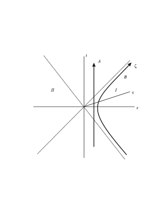
\put(-220.0,220.0){}

Figure 1: Rindler spacetime diagram: A uniformly accelerated observer B (firm B) moves on a hyperbola with acceleration $a$ in region $I$ and is causally disconnected from region $II$.

where $\theta$ is a measure of entanglement. The state is maximally entangled at $\theta=\frac{\pi}{4}$. The first entry in each ket of Eq. (1) corresponds to firm $A$ and the second entry corresponds to firm $B$. From the accelerated firm $B$’s frame, the Minkowski vacuum state is found to be a two-mode squeezed state [14]

$$|0\rangle_{M}=\cos r|0\rangle_{I}|0\rangle_{II}+\sin r|1\rangle_{I}|1\rangle_{II},$$ (2)

where $\cos r=\left(e^{-2\pi\omega c/a}+1\right)^{-1/2}$. The constant $\omega$, $c$ and $a$, in the exponential stand, respectively, for Dirac particle’s frequency, light’s speed in vacuum and firm $B$’s acceleration. In Eq. (2) the subscripts $I$ and $II$ of the kets represent the Rindler modes in region $I$ and $II$, respectively, in the Rindler spacetime diagram (see Fig. ($1$)). The excited state in Minkowski spacetime is related to Rindler modes as follow [14]

$$|1\rangle_{M}=|1\rangle_{I}|0\rangle_{II}.$$ (3)

In terms of Minkowski modes for firm $A$ and Rindler modes for firm $B$, the entangled initial state of Eq. (1) by using Eqs. (2) and (3) becomes

$$|\psi\rangle_{A,I,II}=\cos\theta\cos r|0\rangle_{A}|0\rangle_{I}|0\rangle_{II}+\cos\theta\sin r|0\rangle_{A}|1\rangle_{I}|1\rangle_{II}+\sin\theta|1\rangle_{A}|1\rangle_{I}|0\rangle_{II}.$$ (4)

Since firm $B$ is causally disconnected from region $II$, we must take trace over all the modes in region $II$. This leaves the following density matrix between the two firms,

$$\rho_{A,I}=\left(\begin{array}[]{cccc}\cos^{2}r\cos^{2}\theta&0&0&\cos r\cos\theta\sin\theta\\ 0&\cos^{2}\theta\sin^{2}r&0&0\\ 0&0&0&0\\ \cos r\cos\theta\sin\theta&0&0&\sin^{2}\theta\end{array}\right).$$ (5)

In the quantum Stackelberg duopoly, each firm has two possible strategies $I$, the identity operator and $C$, the inversion operator or Pauli’s bit-flip operator. Let $x$ and $1-x$ stand for the probabilities of $I$ and $C$ that firm $A$ applies and $y$, $1-y$, are the probabilities that firm $B$ applies, respectively. The final density matrix is given by [25]

$$\rho_{f} = xyI_{A}\otimes I_{B}\ \rho_{A,I}\ I_{A}^{{\dagger}}\otimes I_{B}^{{\dagger}}+x\left(1-y\right)I_{A}\otimes C_{B}\ \rho_{A,I}\ I_{A}^{{\dagger}}\otimes C_{B}^{{\dagger}}$$ (6)

$$+y\left(1-x\right)C_{A}\otimes I_{B}\ \rho_{A,I}\ C_{A}^{{\dagger}}\otimes I_{B}^{{\dagger}}$$

$$+\left(1-x\right)\left(1-y\right)C_{A}\otimes C_{B}\ \rho_{A,I}\ C_{A}^{{\dagger}}\otimes C_{B}^{{\dagger}},$$

where $\rho_{A,I}$ is the density matrix given by Eq. (5).

Suppose that the players’ moves in the quantum Stackelberg duopoly are given by probabilities lying in the range $[0,1]$. In the classical form of the duopoly, the moves of firms $A$ and $B$ are given by quantities $q_{1}$ and $q_{2}$, which have values in the range $[0,\infty)$. We assume that firms $A$ and $B$ agree on a function that uniquely defines a real positive number in the range $(0,1]$ for every quantity $q_{1}$, $q_{2}$ in $[0,\infty)$. Such a function is given by $1/(1+q_{i})$, so that firms $A$ and $B$ find $x$ and $y$, respectively, as

$$x=\frac{1}{1+q_{1}}\mathrm{,\qquad}y=\frac{1}{1+q_{2}}$$ (7)

The payoffs of firms $A$ and $B$ are given by the following trace operations

$$P_{A}\left(q_{1},q_{2}\right)=\mathrm{Tr}\left[\rho_{f}P_{A}^{\mathrm{op}}\left(q_{1},q_{2}\right)\right]\mathrm{,\qquad}P_{B}\left(q_{1},q_{2}\right)=\mathrm{Tr}\left[\rho_{f}P_{B}^{\mathrm{op}}\left(q_{1},q_{2}\right)\right],$$ (8)

where $P_{A}^{\mathrm{op}}$, $P_{B}^{\mathrm{op}}$ are payoff operators of the firms and are given by

$$P_{A}^{\mathrm{op}}\left(q_{1},q_{2}\right) = \frac{q_{1}}{q_{12}}\left(k\rho_{11}-\rho_{22}-\rho_{33}\right),$$

$$P_{B}^{\mathrm{op}}\left(q_{1},q_{2}\right) = \frac{q_{2}}{q_{12}}\left(k\rho_{11}-\rho_{22}-\rho_{33}\right),$$ (9)

where $\rho_{ii}$ are the diagonal elements of the final density matrix, $k$ is a constant as given in Ref. [20] and $q_{12}$ is given by

$$q_{12}=\frac{1}{\left(1+q_{1}\right)\left(1+q_{2}\right)}.$$ (10)

The backward-induction outcome in the Stackelberg duopoly is found by first finding the reaction function $R_{2}\left(q_{1}\right)$ of firm $B$ to an arbitrary quantity $q_{1}$ chosen by firm $A$. It is found by differentiating firm $B$’s payoff with respect to $q_{2}$, and maximizing the result for $q_{1}$ and can be written as

$$R_{2}\left(q_{1}\right)=\max P_{B}\left(q_{1},q_{2}\right)$$ (11)

Once firm $B$ chooses this quantity, firm $A$ can compute its optimization problem by differentiating its own payoff with respect to $q_{1}$ and then maximizing it to find the value $q_{1}=q_{1}^{\ast}$. Using the value of $q_{1}^{\ast}$ in Eq. (11), we can get the value of $q_{2}^{\ast}$. These quantities define the backward-induction outcome of the quantum Stackelberg duopoly and represent the subgame perfect Nash equilibrium. The payoffs of the firms at the subgame perfect Nash equilibrium can be found using Eq. (8).

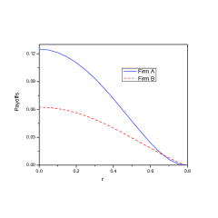
\put(-220.0,220.0){}

Figure 2: (color online) The payoffs are plotted at the subgame perfect Nash equilibrium against the acceleration $r$ for unentangled initial state. The value of $k$ is set to $1$. The solid line represents the payoff of firm $A$ and the dotted line represents the Payoff of firm $B$.

The subgame perfect Nash equilibrium outcome of the duopoly becomes

$$q_{1}^{\ast} = \frac{\cos^{2}\theta(k\cos^{2}r-\sin^{2}r)}{2(\cos^{2}r\cos^{2}\theta+\sin^{2}\theta)}$$

$$q_{2}^{\ast} = \frac{4\cos^{2}\theta(k\cos^{2}r-\sin^{2}r)(\cos^{2}r\cos^{2}\theta+\sin^{2}\theta)}{\begin{array}[]{c}(3-k+12\cos 2r+(1+k)\cos 4r)\cos^{4}\theta\\ -8\cos^{2}\theta((-4+k^{2})\cos^{2}r+k\sin^{2}r)\sin^{2}\theta+16\sin^{4}\theta\end{array}}$$ (14)

It is important to note that the result of Eq. (14) for unentangled initial state ($\theta=0$) reduces to the classical result when we put the acceleration $r=0$. Similarly the results of Ref. [21] for the maximal entangled initial state are retrieved for $\theta=\pi/4$ and $r=0$. In the classical form of the duopoly the subgame perfect Nash equilibrium is a point, whereas in this case, it is a function of both entanglement angle $\theta$ and the acceleration $r$ of firm $B$’s frame. The payoffs of the firms at the subgame perfect Nash equilibrium for unentangled initial state, when $k=1$, are given as

$$P_{A} = \frac{1}{8}\cos^{2}2r\sec^{2}r$$

$$P_{B} = \frac{\cos^{2}r\cos 2r}{4(3+\cos 2r)}$$ (15)

The payoffs of the firms for a maximally entangled initial state, with $k=1$, become

$$P_{A} = \frac{\cos^{2}2r}{8(3+\cos 2r)}$$

$$P_{B} = \frac{\cos^{2}2r(3+\cos 2r)\sec^{2}r}{32(6+\cos 2r)}$$ (16)

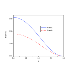
\put(-220.0,220.0){}

Figure 3: (color online) The payoffs are plotted at the subgame perfect Nash equilibrium against the acceleration $r$ for maximally entangled initial state. The value of $k$ is set to $1$. The solid line represents the payoff of firm $A$ and the dotted line represents the Payoff of firm $B$.

The existence of the Nash equilibrium requires that the firms’ moves ($q_{1}^{\ast}$ and $q_{2}^{\ast}$) should have positive values. It can easily be checked from Eq. (14) that for both unentangled and maximally entangled initial states the move of firm $A$ becomes negative for $r\geq\pi/4$. Hence no Nash equilibrium exists for the values of $r$ at which $q_{1}^{\ast}$ becomes negative. Thus the range of the acceleration in which the acceleration parameter $r$ is given by $\pi/4\leq r\leq\pi/2$ is not a physically meaningful range for the Stackelberg duoply. To see how the payoffs are influenced by the acceleration in its physically meaningful range, we plot it against the acceleration parameter $r$. In Fig. $2$, we show the plot of the firms’ payoffs against $r$ for the unentangled initial state. It can be seen that for smaller values of the acceleration, the duopoly is leader advantage and the payoffs decrease with the increasing value of the acceleration. At $r=0.66$ there happens a critical point at which both firms are equally benefitted. From this point onward, the payoff of firm $A$ rapidly decreases and becomes zero at $r=0.76$. The duopoly becomes follower advantage in the region $0.66<r<0.78$. The payoff of the follower firm reaches zero at $r=0.78$. The payoffs of the firms for the maximally entangled initial state are plotted in Fig. $3$. It can be seen that the payoffs of the firms are highly damped as compared to the case of unentangled initial state and the duopoly is follower advantage for the whole range of the acceleration in which the Nash equilibrium exists. The payoffs of both firms becomes zero at $r=0.75$. In Fig. $4$, we plot the payoffs of the firms against the entanglement angle $\theta$. It is seen that the payoffs decrease with the increasing degree of entanglement in the initial state. The duopoly is follower advantage for smaller value of $\theta$ and becomes leader advantage as the degree of the initial state entanglement increases.

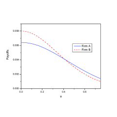
\put(-220.0,220.0){}

Figure 4:  (color online) The payoffs are plotted at the subgame perfect Nash equilibrium against the entanglement angle $\theta$. The values other parameters are chosen as $k=1$, $r=2\pi/9$. The solid line represents the payoff of firm $A$ and the dotted line represents the Payoff of firm $B$.

In conclusion, we study the influence of Unruh effect on the payoffs function of the quantum Stackelberg duopoly. We have shown that the Unruh effect limits the validation of the subgame perfect Nash equilibrium outcome to certain range of acceleration of firm $B$’s frame. The acceleration damps the payoffs function both for unentangled and entangled initial states. However, the damping is heavy when the initial state is maximally entangled and the duopoly always benefit the firm that moves first. For an unentangled initial state, a critical point that correspond to a particular value of the acceleration exists at which both firms are equally benefitted. For larger values of acceleration the duopoly becomes a follower advantage. We show that irrespective of the degree of entanglement in the initial state, the payoffs function vanish when the acceleration of firm $B$ frame reaches to $\pi/4$.

Acknowledgment

Salman Khan is thankful to World Federation of Scientists for partially supporting this work under the National Scholarship Program for Pakistan.

Figures Captions
Figure $1$. Rindler spacetime diagram: A uniformly accelerated observer firm $B$ ($B$) moves on a hyperbola with acceleration $a$ in region $I$ and is causally disconnected from region $II$.
Figure $2$. (color online) The payoffs are plotted at the subgame perfect Nash equilibrium against the acceleration $r$ for unentangled initial state. The value of $k$ is set to $1$. The solid line represents the payoff of firm $A$ and the dotted line represents the Payoff of frim $B$.
Figure $3$. (color online) The payoffs are plotted at the subgame perfect Nash equilibrium against the acceleration $r$ for maximally entangled initial state. The value of $k$ is set to $1$. The solid line represents the payoff of firm $A$ and the dotted line represents the Payoff of frim $B$.
Figure $4$. (color online) The payoffs are plotted at the subgame perfect Nash equilibrium against the entanglement angle $\theta$. The values other parameters are chosen as $k=1$,$r=2\pi/9$. The solid line represents the payoff of firm $A$ and the dotted line represents the Payoff of frim $B$.

References

- [1] von Neumann J 1951 Appl. Math. Ser. 12 36
- [2] Piotrowski E W, Sladkowski J 2002 Physica A 312 208
- [3] Baaquie B E 2001 Phys. Rev. E 64
- [4] Nielson M A ,Chuang I L 2000 Quantum Computation and Quantum Information ( Cambridge: Cambridge University Press)
- [5] Eisert J, Wilkens M and Lewenstein M 1999 Phy. Rev. Lett 83 3077
- [6] Benjamin S C and Hayden P M 2001 Phys. Rev. Lett. 87 0689801
- [7] Marinatto L and Weber T 2001 Phys. lett. A 280 249
- [8] Flitney A P and Abbott D 1999 Phys. Rev. A 65 062318
- [9] Lo C F and Kiang D 2003 Phys. Lett. A 318 333
- [10] Meyer D A 1999 Phys. Rev. Lett. 82 1052
- [11] Cheon T and Tsutsui I 2006 Phys. Lett. A 348 147
- [12] Ichikawa T and Tsutsui I 2007 Ann. Phys. 322 531
- [13] Ichikawa T, Tsutsui I and Cheon T 2008 J. Phys. A: Math. Theor. 41 135303
- [14] Alsing P M, Fuentes-Schuller I, Mann R B and Tessier T E 2006 Phys. Rev. A 74 032326.
- [15] Ling Y et al 2007 J. Phys. A: Math. Theor. 40 9025.
- [16] Gingrich R M and Adami C 2002 Phys. Rev. Lett. 89 270402.
- [17] Pan Q and Jing J 2008 Phys. Rev. A 77 024302.
- [18] Fuentes-Schuller I and Mann R B 2005 Phys. Rev. Lett. 95 120404.
- [19] Terashima H and Ueda M 2003 Int. J. Quantum Inf. 1 93.
- [20] Gibbons R 1992 Game theory for Applied Economists (Princeton University Press, Princeton, NJ)
- [21] Iqbal A and Toor A H 2002 Phys. Rev. A 65 052328
- [22] Zhu X and Kuang L M 2007 J. Phys. A: Math. Theor. 40 7729
- [23] Zhu X and Kuang L M 2008 Commun. Theor. Phys. 49 111
- [24] Khan S, Ramzan M and Khan M K 2010 J. Phys. A: Math. Theor. 43 375301
- [25] Marinatto L and Weber T 2000 Phys. Lett. A 272 291