Electron density fluctuations accelerate the branching of streamer discharges in air

Abstract

Branching is an essential element of streamer discharge dynamics but today it is understood only qualitatively. The variability and irregularity observed in branched streamer trees suggest that stochastic terms are relevant for the description of streamer branching. We here consider electron density fluctuations due to the discrete particle number as a source of stochasticity in positive streamers in air at standard temperature and pressure. We derive a quantitative estimate for the branching distance that agrees within a factor of 2 with experimental values. As branching without noise would occur later, if at all, we conclude that stochastic particle noise is relevant for streamer branching in air at atmospheric pressure.

Streamers are filamentary electrical discharges that propagate through a non-conducting medium when it is suddenly exposed to a high electric field Raether1939/ZPhy . As first stages of electrical breakdown Raizer1991/book , they are found in nature preceding a lightning stroke and as the building blocks of upper-atmospheric discharges above thunderstorms Franz1990/Sci ; Pasko2003/Natur ; *Pasko1998/GeoRL/1; Ebert2010/JGRA/c . Due to their efficient production of chemical radicals Winands2006/JPhD , streamers are used in industry for gas cleaning and sterilization.

Streamer discharges frequently form irregular trees with many branches both in laboratory, where branch length and branching angles in air have been measured recently Briels2008/JPhD ; Nijdam2008/ApPhL , and in upper-atmospheric discharges McHarg2010/JGRA/c . However, our present understanding of streamer branching is only qualitative. Streamer trees in the laboratory are highly random and irregular but simulations have shown that streamers can branch even in fully deterministic density models Arrayas2002/PhRvL ; Montijn2006/PhRvE ; Liu2006/JPhD ; Babaeva2008/ITPS . Model reduction and analytical theory explained branching as a Laplacian instability that develops when the space charge layer around the streamer head is much thinner than the streamer radius Ebert2011/Nonli . Nevertheless, the analysis of a reduced moving-boundary streamer model suggests that streamer heads are linearly stable Tanveer2009/PhyD ; Kao2010/PhyD even if the stabilizing effects of electron diffusion and photo-ionization are neglected. Streamer fingers are therefore similar to laminar pipe flow: a finite perturbation is required to let streamers branch or to make the pipe flow turbulent.

A small, but finite perturbation to trigger branching can be due to the initial condition. But it can also be created by fluctuations during the evolution. Such fluctuations are naturally included in Monte Carlo models Moss2006/JGRA ; Chanrion2008/JCoPh ; *Chanrion2010/JGRA/c; Li2009/JPhD ; *Li2010/JCoPh; *Li2011/arXiv that follow the single electron motion; they model the stochastic distribution of electron positions and energies. Those models are microscopically very accurate at the cost of high computational demands. Even state-of-the art spatially hybrid codes Li2009/JPhD ; *Li2010/JCoPh; *Li2011/arXiv are still limited to quite short streamers.

Here we introduce a new computational model and present its quantitative predictions for positive streamers in air at standard temperature and pressure. The model is a spatially extended stochastic model Gardiner2004/book that assumes an electron energy distribution determined by the local electric field but accounts for density fluctuations due to the discrete number of electrons. Since particles are not individually tracked, the required memory and computations are roughly independent of the number of active particles, in contrast to Monte Carlo methods. We study the evolution towards branching with realistic density fluctuations in full three dimensions and, extrapolating, obtain branching ratios that are consistent with the experiments Briels2008/JPhD ; Nijdam2008/ApPhL . This suggests that streamer branching in air at atmospheric pressure is triggered by electron density fluctuations.

Model.- The most relevant microscopic processes in streamers are two-body reactions between free electrons and neutral gas molecules. Therefore most quantities of a streamer discharge scale with the neutral gas density in a definite manner called Townsend scaling Ebert2010/JGRA/c . Following Ebert2006/PSST we define a typical length for streamers in air $l_{0}\approx 2.3\,\mathrm{\mu m}\cdot(N_{0}/N)$, a typical electric field $E_{0}\approx 2\cdot 10^{5}\,\mathrm{V/cm}\cdot(N_{0}/N)$ a typical time $t_{0}=3\cdot 10^{-12}\,\mathrm{s}\cdot(N_{0}/N)$ and a typical density of charge carriers $n_{0}\equiv\epsilon_{0}E_{0}/\mathrm{e}l_{0}\approx 4.7\cdot 10^{14}\,\mathrm{cm^{-3}}\cdot(N_{0}/N)^{2}$, where $\mathrm{e}$ is the elementary charge, $N$ is the molecule number density of air and $N_{0}$ is the number density at standard pressure and temperature, used as an arbitrary reference. We refer to Ebert2010/JGRA/c for a physical interpretation of these quantities and scaling laws.

Using these typical magnitudes one can build a dimensionless streamer model. We consider here a minimal model for air Ebert2006/PSST ; Wormeester2010/arXiv that also includes photo-ionization Luque2007/ApPhL . We are interested on the dynamics of the streamer head, where impact ionization strongly dominates over electron removal by dissociative attachment and the latter can be safely neglected. The governing equations are therefore

$$\partial_{t}\sigma = D\nabla^{2}\sigma+\mathbf{\nabla}\cdot(\sigma{\bf E})+S^{(ph)}+S^{(impact)},$$ (1)

$$\partial_{t}\rho = S^{(ph)}+S^{(impact)},$$ (2)

$$\nabla^{2}\phi = \sigma-\rho,~{}~{}~{}{\bf E}=-\mathbf{\nabla}\phi.$$ (3)

Here $\sigma$ and $\rho$ are the (dimensionless) electron and ion densities, $S^{(ph)}$ and $S^{(impact)}$ are, respectively, the photo-ionization and impact ionization sources of electron-ion pairs, $\phi$ is the electrostatic potential ${\bf E}$ the electric field, and $D$ is a diffusion coefficient, taken as $D=0.1$.

There are several corrections to Townsend scaling Ebert2010/JGRA/c . One arises from collisional quenching of photo-ionization Liu2006/JPhD , here included in $S^{(ph)}$, which contains an explicit dependence on the air density. A second correction, on which we focus here, arises from the finite number of particles and the stochastic nature of microscopic processes; this cannot be expressed in equations (1)-(3), because they only contain macroscopic quantities. Rather we will take a discretization of (1)-(3) and convert it into a spatially extended stochastic modelGardiner2004/book .

Method.- Since the importance of stochastic noise depends on the particle number density our first step is to derive, from the magnitudes described above, a dimensionless parameter for the typical number of charge carriers contained in a typical volume. We define $g\equiv n_{0}l_{0}^{3}=E_{0}\varepsilon_{0}l_{0}^{2}/\mathrm{e}$. This is the number of elementary charges that has to sit in each area $l_{0}^{2}$ of an infinite charged plane to create a jump $E_{0}$ in the electric field. In air $g\approx 5700\cdot(N_{0}/N)$; at an altitude of $70\,\mathrm{km}$, typical for sprites, $g\approx 10^{8}$.

The relative amplitude of the statistical fluctuations of a number $g$ of particles is $g^{-1/2}$. The limit of negligible fluctuations is $g^{-1/2}\ll 1$. In air at atmospheric pressure, $g^{-1/2}\approx 0.01$ and stochastic noise is a relatively small correction on the fluid description. However, as we will see, due to the strongly nonlinear nature of streamer discharges, such small fluctuations can be amplified by strong electric fields and alter significantly the propagation of a streamer. For sprites, $g^{-1/2}$ is much smaller, about $10^{-4}$.

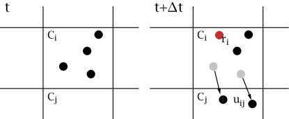
Figure 1: Scheme of an elementary time-step in the lattice model. Each electron is represented here by a dot; note however that we do not keep track of every individual particle: only the number of particles in each cell. During the time-step from $t$ to $t+\Delta t$ we move $u_{ij}$ electrons from cell $C_{i}$ to $C_{j}$. Meanwhile, $r_{i}$ electrons arise in $C_{i}$ from impact ionization and photo-ionization.

Now let us take a spatial discretization of (1)-(3): the simulation domain (see Fig.1) is divided into cells $C_{i}$, each with a dimensionless volume $v_{i}=V_{i}/l_{0}^{3}$ ($V_{i}$ is the dimensional volume). If we are given the dimensionless densities in each cell, $\sigma_{i}$ and $\rho_{i}$, we know, from our discretization, how to calculate the left hand sides of (1)-(3). In particular, we can calculate the source term $S_{i}=S^{(ph)}_{i}+S^{(impact)}_{i}$ and the flux from cell $C_{i}$ to each neighboring cell $C_{j}$, which we denote $F_{ij}$.

But instead of densities one has a discrete number of electrons and ions in each cell, $N^{(e)}_{i}$ and $N^{(i)}_{i}$; the dimensionless densities are therefore $\sigma_{i}=N^{(e)}_{i}/n_{0}V_{i}=N^{(e)}_{i}/gv_{i}$, $\rho_{i}=N^{(i)}_{i}/gv_{i}$. We may now use these to calculate the source terms and the fluxes. The problem is now how to update the number of particles as time evolves. To simplify the description, let us first describe a time-stepping that will tend to a forward Euler discretization with time step $\Delta t$.

We look first at the source terms. Let $r_{i}$ be the number of electron-ions pairs created in $C_{i}$ during a time $\Delta t$. This quantity follows a Poisson distribution with average $\lambda_{i}=gv_{i}S_{i}\Delta t$. So in the simulation we draw for each $i$ a sample from the Poisson probability distribution $p(r_{i})=\lambda_{i}^{r_{i}}e^{-\lambda_{i}}/r_{i}!$.

The transport terms are slightly more complicated because the number of electrons must be conserved. We interpret the $gv_{i}F_{ij}\Delta t$ as the average number of electrons that flows from $C_{i}$ to $C_{j}$ during $\Delta t$ (note that $F_{ij}\neq F_{ji}$). Thus the probability for an electron in $C_{i}$ at $t$ to end in $C_{j}$ at $t+\Delta t$ is $p_{ij}=N^{(e)}_{i}F_{ij}\Delta t/gv_{i}$ for $i\neq j$. But since the electron must end somewhere, $p_{ii}=1-\sum_{j\neq i}p_{ij}$ . We can use these $p_{ij}$ to obtain the number of electrons moving from $C_{i}$ to $C_{j}$, that we denote $u_{ij}$. The probability distribution for the electrons exiting $C_{i}$ is the multinomial distribution with $\sum_{j}u_{ij}=N^{(e)}_{i}$.

Now we have all the ingredients to update the particle numbers as

$$N^{(e)}_{i}(t+\Delta t)=N^{(e)}_{i}(t)+r_{i}+\sum_{j}\left(u_{ji}-u_{ij}\right)$$ (4)

As mentioned above, this scheme tends to an explicit Euler time discretization of the fluid equations as $g^{-1/2}\to 0$. But we can also design a two-step time updating that tends to second order Runge-Kutta Montijn2006/JCoPh if we (a) use the particle numbers at $t$ to calculate $S_{i}(t)$ and $F_{ij}(t)$, (b) perform a half-step using $\Delta t/2$ to update the particle numbers, (c) use the new particle numbers to obtain $S_{i}(t+\Delta t/2)$ and $S_{i}(t+\Delta t/2)$ (c) define $S^{\prime}_{i}(t)=(S_{i}(t)+S_{i}(t+\Delta t))/2$, $F^{\prime}_{ij}(t)=(F_{ij}(t)+F_{ij}(t+\Delta t))/2$ and use them to perform a step $\Delta t$. Note that in principle step (b) could also implement a standard continuum step, since nothing forces us to preserve an integer number of particles in that intermediate step; we opted however to use the same stochastic step in both stages of the algorithm.

We have not yet mentioned the spatial discretization to calculate $F_{ij}$. The reason is that the scheme is flexible on that. We used here the scheme described in Montijn2006/JCoPh . This is a flux-limited, nonlinear discretization schemes and it poses an additional difficulty: it sometimes leads to negative $F_{ij}$ which cannot be interpreted as a probability. In that case, we rearrange the fluxes by letting $F_{ij}\to F^{\prime}_{ij}$, with $F^{\prime}_{ij}=0$, $F^{\prime}_{ji}=F_{ji}-F_{ij}$ until no negative fluxes remain.

Results.- We now use the adaptive grid refinement and the fluxes and reaction terms from Montijn2006/JCoPh and the three-dimensional cylindrical mesh of Ref. Luque2008/PhRvL . As a first application, let us analyze the initiation of breakdown in a small plane-to-plane geometry with a potential difference of $16\,\mathrm{kV}$ between two electrodes separated by 2 mm of air. The simulated volume is discretized into cells $\Delta r=\Delta z=8\,\mathrm{\mu m}$, $\Delta\theta=2\pi/64$. As initial condition, we set a neutral hemispherical gaussian seed at $z=r=0$ (positive electrode) containing $\sim 6\cdot 10^{5}$ electrons.

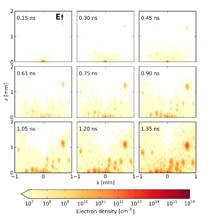
Figure 2: Snapshots of the cross section of the electron density in the $y=0$ plane in a plane-plane, 2 mm gap with a potential difference of 16 kV. Multiple avalanches start out of seeds produced by photo-ionization; the electric breakdown extends to the complete volume and no actual streamer is initiated. A movie of this simulation is available in the auxiliary material.

Figure 2 shows the evolution of a cross-section of the electron densities up to $1.35\,\mathrm{ns}$. In that short time-span, a multitude of avalanches seeded by photo-ionization has developed. A very similar evolution is observed in the Monte Carlo simulations of Li2011/arXiv ; both results show that in strong electric fields noise weakens or even prevents the formation of streamers.

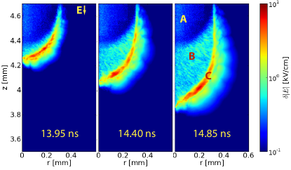
Figure 3: Highest deviation of the absolute value of the electric field from its azimuthal average at three snapshots. The volume labelled A corresponds to the evolution of the streamer up to $t=13.5\,\mathrm{ns}$, with noise switched off. When we switch on noise, the streamer body (B) develops low-amplitude, small-scale fluctuations. The streamer surface close to the tip (C) has fluctuations with a higher amplitude and an auto-correlation length of about one tenth of a millimeter. The amplitude grows but in this simulation it remains small small compared with values of some hundreds of kV/cm in that area.

The situation changes however for a streamer in a point-plane geometry. Then only in a small volume is the electric field high enough to produce significant ionization.

We run a simulation with point-plane electrodes implemented as in Luque2008/JPhD . The needle is $2\,\mathrm{mm}$ long and its tip is separated from the plate by $7.2\,\mathrm{mm}$. As initial condition we set a semi-spherical neutral gaussian ionization seed at the needle tip with a radius of $73.6\,\mathrm{\mu m}$ and a peak ionization density of $4.7\cdot 10^{18}\,\mathrm{cm^{-3}}$. The needle has a positive potential of $10.5\,\mathrm{kV}$ relative to the lower electrode. We used an adptive refinement strategy Montijn2006/JCoPh with coarsest grid $\Delta z=\Delta r=40\,\mathrm{\mu m}$ and finest grid $\Delta z=\Delta r=2.5\,\mathrm{\mu m}$ . Since full 3d simulations are too demanding, we chose to run the simulation with cylindrical symmetry and $g^{-1/2}=0$ up to $t=13.5\,\mathrm{ns}$. Then we remove the constraint of cylindrical symmetry and introduce stochastic noise at the level expected at atmospheric pressure ($g=5700$). The continuous density at each cell is then interpreted as an average and discrete numbers of particles are obtained by drawing random samples from a Poisson distribution with this average.

To represent the evolution of this 3d simulation that deviates only slightly from perfect cylindical symmetry, let us consider the average of some quantity around the azimuthal angle, $\langle u\rangle_{\theta}=\frac{1}{2\pi}\int_{0}^{2\pi}u(r,z,\theta)d\theta$. The deviation from symmetry can then be defined as $\delta u=\max_{\theta}(u-\langle u\rangle_{\theta})$. Figure 3 shows $\delta|E|$ at three instants of time after noise is introduced into the simulation.

This simulation is highly demanding: the short streamer evolution represented in Fig. 3 took about 5 weeks using two dual-core 3 GHz AMD Opteron processors. We could not run the simulation long enough to observe actual branching; nevertheless, we can use the present result for a first quantitative estimation of the time needed to branch.

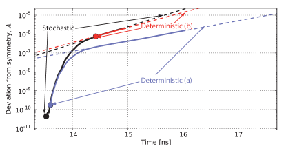
Figure 4: Evolution of $A$ as defined in the text. We show the evolution of three runs: in all runs the system was deterministic and cylindrically symmetrical up to time 13.5 ns. After this point we add stochasticity and allow deviations from cylindrical symmetry. In the curves marked as deterministic, we remove noise again at the time marked with the dots while keeping the unsymmetric perturbations that have evolved up to that time. Within this limited timeframe, $A$ seems go through a transient, fast growth phase until it settles into an exponential growth. The dashed line fits this second phase. For the completely stochastic run the best fit is $A=ae^{t/\tau}$ with $a=5\cdot 10^{-20}$, $\tau=0.48\,\mathrm{ns}$. Extrapolating, this predicts branching at $t\sim-\tau\log a\approx 21\,\mathrm{ns}$.

Let us look at the Fourier transform of the electron density $\sigma$ along the azimuthal coordinate $\theta$, $\tilde{\sigma}(r,z,k)=\frac{1}{2\pi}\int_{0}^{2\pi}d\theta n_{e}(r,z,\theta)e^{-ik\theta}$. We can define the “total spectral content” of mode $k$ of the electron density as $W_{k}=2\pi\int_{-\infty}^{+\infty}dz\,\int_{0}^{\infty}dr\,r\tilde{\sigma}(r,z,k)$. If the streamer is close to cylindrical symmetry (i.e. it is far from a branching state), $|W_{0}|\gg|W_{k}|$ for all $k>0$. Hence if we define $A=\sum_{k>0}|W_{k}|^{2}/|W_{0}|^{2}$ we can postulate that the condition for branching is $A\sim 1$.

In Figure 4 the value of $A$ during the simulated time frame is plotted as a black line. During the full evolution we find $A\ll 1$, i.e. the streamer was at all times far from branching. However we can use $A(t)$ to obtain a first estimation of the branching time. After a transient, $A$ growths exponentially; extrapolating this growth to $A\sim 1$ we can roughly estimate the branching time as $t_{branch}\sim 21\,\mathrm{ns}$. The streamer velocity is approximately $v=0.32\,\mathrm{mm/ns}$ and hence after the introduction of noise the streamer would run for about $2.4\,\mathrm{mm}$ before branching. The measurements in Briels2008/JPhD ; Nijdam2008/ApPhL give a ratio of the branching distance to the streamer diameter of about 12-15. This is relative to the radiative diameter, estimated to be about half of the electrodynamic diameter Pancheshnyi2005/PhRvE ; with that estimation, our value is about 8. One must also take into account that (a) short branching distances are harder to measure and therefore the average in Briels2008/JPhD ; Nijdam2008/ApPhL may be slightly overestimated and (b) both in our model and in observations branching distance is random: we are comparing the result of only one simulation with an average over many measurements so a certain discrepancy seems natural.

However, our estimation of a branching distance is close to the measured value, suggesting that noise resulting from the finite number of particles is relevant in streamer discharges. To measure the relevance of a persisting noise compared with the inherent growth of cylindrically perturbed modes we performed two simulations in which noise is removed after some time. These are shown in the two curves of Figure 4 labelled as deterministic (a) and (b). We see that noise always increases the growth rate of the deviations but also that even a relatively small amount of noise during a short time (a) is enough to trigger an instability that would eventually lead to streamer branching. Longer simulations must be performed to check that the evolution suggested in Fig. 4 continues until the streamer branches.

Note that at lower pressure, such as those in the high layers of the atmosphere where sprite streamers are commonly observed, stochastic noise is weaker ($g^{-1/2}\approx 10^{-4}$). Although the ratio between diameter and branching distance has not yet been measured in sprites, they also branch frequently McHarg2010/JGRA/c . However, in the upper atmosphere, other sources of stochasticity may be relevant, such as cosmic rays and atmospheric inhomogeneities.

- (1) H. Raether, Zeitschrift fur Physik 112, 464 (1939)
- (2) Y. P. Raizer, Gas Discharge Physics (Springer-Verlag, Berlin, Germany, 1991)
- (3) R. C. Franz, R. J. Nemzek, and J. R. Winckler, Science 249, 48 (1990)
- (4) V. P. Pasko, Nature (London) 423, 927 (2003)
- (5) V. P. Pasko, U. S. Inan, and T. F. Bell, Geophys. Res. Lett. 25, 2123 (1998)
- (6) U. Ebert, S. Nijdam, C. Li, A. Luque, T. Briels, and E. van Veldhuizen, J. Geophys. Res. (Space Phys) 115, A00E43 (2010), arXiv:1002.0070
- (7) G. J. J. Winands, Z. Liu, A. J. M. Pemen, E. J. M. van Heesch, K. Yan, and E. M. van Veldhuizen, J. Phys. D 39, 3010 (2006)
- (8) T. M. P. Briels, E. M. van Veldhuizen, and U. Ebert, J. Phys. D 41, 234008 (2008), arXiv:0805.1364
- (9) S. Nijdam, J. S. Moerman, T. M. P. Briels, E. M. van Veldhuizen, and U. Ebert, Appl. Phys. Lett. 92, 101502 (2008), arXiv:0802.3639
- (10) M. G. McHarg, H. C. Stenbaek-Nielsen, T. Kanmae, and R. K. Haaland, J. Geophys. Res. (Space Phys) 115, A00E53 (2010)
- (11) M. Arrayás, U. Ebert, and W. Hundsdorfer, Phys. Rev. Lett. 88, 174502 (2002), nlin/0111043
- (12) C. Montijn, U. Ebert, and W. Hundsdorfer, Phys. Rev. E 73, 065401 (2006), physics/0604012
- (13) N. Liu and V. P. Pasko, J. Phys. D 39, 327 (2006)
- (14) N. Y. Babaeva and M. J. Kushner, IEEE Trans. Plasma Sci. 36, 892 (2008)
- (15) U. Ebert, F. Brau, G. Derks, W. Hundsdorfer, C. Kao, C. Li, A. Luque, B. Meulenbroek, S. Nijdam, V. Ratushnaya, L. Schäfer, and S. Tanveer, Nonlinearity 24, 1 (2011)
- (16) S. Tanveer, L. Schäfer, F. Brau, and U. Ebert, Physica D Nonlinear Phenomena 238, 888 (2009), arXiv:0809.0319
- (17) C. Kao, F. Brau, U. Ebert, L. Schäfer, and S. Tanveer, Physica D Nonlinear Phenomena 239, 1542 (2010), arXiv:0908.2521
- (18) G. D. Moss, V. P. Pasko, N. Liu, and G. Veronis, J. Geophys. Res. (Space Phys) 111, 2307 (2006)
- (19) O. Chanrion and T. Neubert, J. Comput. Phys. 227, 7222 (2008)
- (20) O. Chanrion and T. Neubert, J. Geophys. Res. (Space Phys) 115, A00E32 (2010)
- (21) C. Li, U. Ebert, and W. Hundsdorfer, J. Phys. D 42, 202003 (2009), arXiv:0907.0555
- (22) C. Li, U. Ebert, and W. Hundsdorfer, J. Comput. Phys. 229, 200 (2010), arXiv:0904.2968
- (23) C. Li, U. Ebert, and W. Hundsdorfer(2011), arXiv:1101.1189
- (24) C. Gardiner, Handbook of Stochastic Methods: for Physics, Chemistry and the Natural Sciences, 3rd edition (Springer-Verlag, Berlin, Germany, 2004)
- (25) U. Ebert, C. Montijn, T. M. P. Briels, W. Hundsdorfer, B. Meulenbroek, A. Rocco, and E. M. van Veldhuizen, Plasma Sour. Sci. Technol. 15, 118 (2006), physics/0604023
- (26) G. Wormeester, S. Pancheshnyi, A. Luque, S. Nijdam, and U. Ebert(2010), arXiv:1008.3309
- (27) A. Luque, U. Ebert, C. Montijn, and W. Hundsdorfer, Appl. Phys. Lett. 90, 081501 (2007), physics/0609247
- (28) Note that nothing assures us that , although it would be if . The solution that we implemented in that case is to set and renormalize the rest of the such that
- (29) C. Montijn, W. Hundsdorfer, and U. Ebert, J. Comput. Phys. 219, 801 (2006), physics/0603070
- (30) A. Luque, U. Ebert, and W. Hundsdorfer, Phys. Rev. Lett. 101, 075005 (2008), arXiv:0712.2774
- (31) A. Luque, V. Ratushnaya, and U. Ebert, J. Phys. D 41, 234005 (2008), arXiv:0804.3539
- (32) In the adaptive refinement algorithm one has to interpolate densities from coarser to finer grid. We adapted this to our discrete algorithm by interpreting densities as probabilities and again sampling from a multinomial distribution. Thus, all cells contain a discrete number of particles and this number is preserved across nested grids.
- (33) S. Pancheshnyi, M. Nudnova, and A. Starikovskii, Phys. Rev. E 71, 016407 (2005)