On the road towards multidimensional tori.

Abstract

The problem of persistence of four-frequency tori is considered in models represented by the coupled periodically driven self-oscillators. We show that the adding the third oscillator gives rise to destruction of the three-frequency tori, with appearance of regions of either chaotic attractors or four-frequency tori. As the coupling strength decreases, the four-frequency tori dominate, and the amplitude threshold of their occurrence vanishes. Also, for three oscillators, a domain of complete synchronization of the system by the external driving can disappear.

Kotel’nikov’s Institute of Radio-Engineering and Electronics of RAS, Saratov Branch,
Zelenaya 38, Saratov, 410019, Russian Federation.

PACS: 05.45.-a, 05.45.Xt

1 INTRODUCTION

A problem of effect of external driving in systems of mutually coupled self-oscillators is a fundamental part of the theory of synchronization important for a variety of applications [1], [2]. It is a part of a field related to birth and synchronization of multi-frequency quasi-periodic oscillations. In particular, it goes back to the concept of the onset of turbulence advanced by Landau and Hopf, which is based on successive appearance of growing number of quasi-periodic components of the motion with increase of the Reynolds number [3]. As known, further developments of nonlinear dynamics and bifurcation theory have made this hypothesis doubtful in some respects. According to Ruelle and Takens [4], in systems with multiple oscillatory components arising successively due to a sequence of bifurcations, the quasi-periodic motions associated with torus attractors cannot occur as typical at a number of frequency components larger than three; instead a strange attractor should appear. On the other hand, computations for model systems undertaken by several authors do not quite agree with this statement: in certain situations tori of sufficiently high dimension seem persisting and observable [5]. Thus, the question of how the transition to chaos in multidimensional systems develops, and what is the role of the number of oscillatory components, or degrees of freedom, involved in the dynamics, deserve further studies. The phase approximation whereby dynamics of coupled periodically driven self-oscillators is investigated appears to be effective and illuminating in the study of this problem [5]. In this paper, in the framework of the phase equations we discuss transformation of the regions of the different regimes in the parameter space when the number of driven oscillators increases. Thus, we will be interested in the question of how the transition to high-dimensional tori and chaos depends on the number of oscillators in the system. Also, we show that an increase in the number of oscillators up to three leads to a new effect - a domain of complete synchronization may disappear.

2 PHASE EQUATIONS

Let us consider a system of three dissipative coupled van der Pol oscillators driven by an external periodic force (Fig.1):

$$\begin{array}[]{l}\ddot{x}-(\lambda-x^{2})\dot{x}+x+\mu(\dot{x}-\dot{y})=B\sin\omega t,\\ \\ \ddot{y}-(\lambda-y^{2})\dot{y}+(1+\Delta_{1})y+\mu(\dot{y}-\dot{x})+\mu(\dot{y}-\dot{z})=0,\\ \\ \ddot{z}-(\lambda-z^{2})\dot{z}+(1+\Delta_{2})z+\mu(\dot{z}-\dot{y})=0.\end{array}$$ (1)

Here $\lambda$ is a parameter responsible for the Andronov – Hopf bifurcation in the independent oscillators, $\Delta_{1,2}$ are frequency detuning of the second and third oscillators from the first oscillator, $\mu$ is the coupling coefficient, $B$ is an amplitude of the external periodic force, $\omega$ is its frequency. The frequency of the first oscillator is assumed to be normalized to unity.

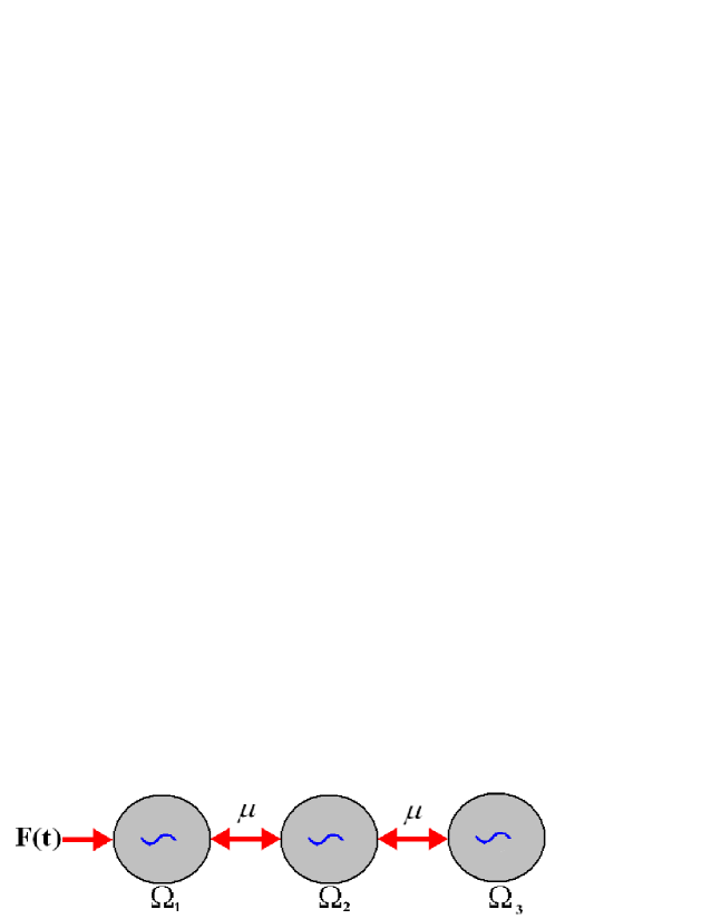
Figure 1: Schematic representation of a system of three dissipative coupled oscillators driven by an external periodic force.

The system (1) may be analyzed in terms of complex amplitudes (quasiharmonic approximation) if the parameter $\lambda$ is small. For this, we set

$$\begin{array}[]{c}x=a(t)e^{i\omega t}+a^{\ast}(t)e^{-i\omega t},\quad y=b(t)e^{i\omega t}+b^{\ast}(t)e^{-i\omega t},\\ \\ z=c(t)e^{i\omega t}+c^{\ast}(t)e^{-i\omega t}.\end{array}$$ (2)

Here, $a$, $b$, $c$ are the complex amplitudes of the oscillators slow varying in time scale of the basic oscillations with unit frequency. We use the additional conditions traditional for this method

$$\begin{array}[]{c}\dot{a}(t)e^{i\omega t}+\dot{a}^{\ast}(t)e^{-i\omega t}=0,\quad\dot{b}(t)e^{i\omega t}+\dot{b}^{\ast}(t)e^{-i\omega t}=0,\\ \\ \dot{c}(t)e^{i\omega t}+\dot{c}^{\ast}(t)e^{-i\omega t}=0.\end{array}$$ (3)

Then, we substitute (2) and (3) in (1), multiply the equations by factor $e^{-i\omega t}$, and perform averaging over a period of the basic oscillations. Assuming $\omega\approx 1$ the resulting equations for complex amplitudes are as follows

$$\begin{array}[]{rl}2\dot{a}=&\lambda a-|a|^{2}a-2i\Omega a-\mu(a-b)-\displaystyle\frac{b}{4},\\ \\ 2\dot{b}=&\lambda b-|b|^{2}b-i(2\Omega-\Delta_{1})b-\mu(b-a)-\mu(b-c),\\ \\ 2\dot{c}=&\lambda c-|c|^{2}c-i(2\Omega-\Delta_{2})c-\mu(c-b),\end{array}$$ (4)

where $\Omega=\omega-1$ is detuning parameter of the external driving force with respect to the first oscillator. Note that in the equations (4) the parameter $\lambda$ may be eliminated via variable change, and then the other parameters will be renormalized with the factor $\lambda^{-1}$ [5]. Let us set $a=Re^{i\psi_{1}}$, $b=re^{i\psi_{2}}$, $c=ve^{i\psi_{3}}$, where $R$, $r$, $v$ are real amplitudes, and $\psi_{1,2,3}$ are phases of the oscillators. Following the Refs. [1], [4], [5], we assume that the motion takes place close to the unperturbed limit cycles of the oscillators, and set $R\approx 1$, $r\approx 1$, $v\approx 1$. Then, the phases have to satisfy the equations

$$\begin{array}[]{rl}\dot{\psi}_{1}=&-\Omega-\displaystyle\frac{1}{2}\mu\sin(\psi_{1}-\psi_{2})+b\sin\psi_{1},\\ &\\ \dot{\psi}_{2}=&-\Omega+\displaystyle\frac{1}{2}\Delta_{1}+\displaystyle\frac{1}{2}\mu\sin(\psi_{1}-\psi_{2})-\displaystyle\frac{1}{2}\mu\sin(\psi_{2}-\psi_{3}),\\ &\\ \dot{\psi}_{3}=&-\Omega+\displaystyle\frac{1}{2}\Delta_{2}+\displaystyle\frac{1}{2}\mu\sin(\psi_{2}-\psi_{3}).\end{array}$$ (5)

Further we shall use the relative phases of the oscillators $\theta=\psi_{1}-\psi_{2}$ and $\varphi=\psi_{2}-\psi_{3}$. Equations (5) generalize the equations obtained in Ref.[4] to the case of three driven oscillators.

3 SYNCHRONIZATION OF TWO-
FREQUENCY OSCILLATIONS

First, let us turn to the case of two oscillators. Then phase equation are

$$\begin{array}[]{rl}\dot{\psi}_{1}=&-\Omega-\displaystyle\frac{1}{2}\mu\sin\theta+b\sin\psi_{1},\\ &\\ \dot{\psi}_{2}=&-\Omega+\displaystyle\frac{1}{2}\Delta_{1}+\displaystyle\frac{1}{2}\mu\sin\theta.\end{array}$$ (6)

We fix the ”internal” parameters of the system $\Delta_{1}=0.3$ and $\mu=0.4$. Obviously, in absence of the external driving $b=0$, the condition of mutual synchronization of the subsystems is $\mu>\displaystyle\frac{\Delta_{1}}{2}$ [1]. Hence, the above selected parameter values correspond to the regime of the mode locking for the unforced system. The external signal applied can destroy this regime.

To visualize the domains of different dynamical regimes the results of parameter scan are represented in Fig.2a for the ($\Omega$, $b$) parameter plane. Shown are the region of complete synchronization of the phases of oscillators by the external driving $P$ and regions of the quasiperiodical regimes, namely, two-frequency tori $T_{2}$ and three-frequency tori $T_{3}$. For each parameter value we perform computations to reach a sustained dynamical regime of the model (6), and then evaluate two Lyapunov exponents, $\Lambda_{1}$ and $\Lambda_{2}$, using a standard Bennettin algorithm. The nature of the regimes is determined as follows. The case $\Lambda_{1}<0$, $\Lambda_{2}<0$ corresponds to a complete phase locking of the oscillator phases by the external force. The cases $\Lambda_{1}=0$, $\Lambda_{2}<0$ and $\Lambda_{1}=\Lambda_{2}=0$ are interpreted as associated with quasiperiodic regimes of two-frequency tori and three-frequency tori, respectively.

It should be noted, that numerical tests are inevitably crude. In particular, some of the points labelled as three-frequency quasiperiodic may well be high-order resonance two-frequency quasiperiodic, and four-frequency quasiperiodic may well be three-frequency quasiperiodic with high-order relation. Furthermore, such a Lyapunov classification labels as quasiperiodic some points, at which the Lyapunov exponent may vanish, for example, bifurcation points, but this situations usually take place only at the borders of domains of stable dynamical regimes and do not influence the overall picture.

The two-frequency regimes $T_{2}$ correspond to a partial locking of the oscillatory system by the external periodic force, while the relative phase oscillates near some stationary value. Observe that these regimes dominate at small driving amplitudes, that is, they occupy a largest area on the parameter plane there. At large amplitudes, again the two-frequency tori occur, but now the first oscillator is partially locked. In the intermediate domain of moderate amplitudes, the three-frequency tori $T_{3}$ are observed, and the region of their occurrence is pierced by narrow tongues of higher order resonance two-frequency tori.

4 SYNCHRONIZATION OF THREE-
FREQUENCY OSCILLATIONS

Now, let us add the third oscillator into the model system, and turn to the complete set of equations (5). We keep the same parameter values $\Delta_{1}=0.3$ and $\mu=0.4$, and set additionally $\Delta_{2}=1$. In the absence of the external force, presence of the third oscillator gives rise to regime of beats at these parameter values. In other words, the third oscillator destroys the mutual mode-locking of the first and second oscillators. As a result, essential complication of the arrangement of domains in the parameter plane ($\Omega$, $b$) is observed.

Fig.2b shows the parameter plane chart for the system of three coupled driven oscillators. Now, the picture is drawn using numerical analysis of three Lyapunov exponents. New formations are observed on the diagram. These are domains of four-frequency tori $T_{4}$, where $\Lambda_{1}=\Lambda_{2}=\Lambda_{3}=0$ (up to numerical errors), and domains of chaos $C$, with one positive exponent, that is $\Lambda_{1}>0$, $\Lambda_{2}<0$, $\Lambda_{3}<0$.

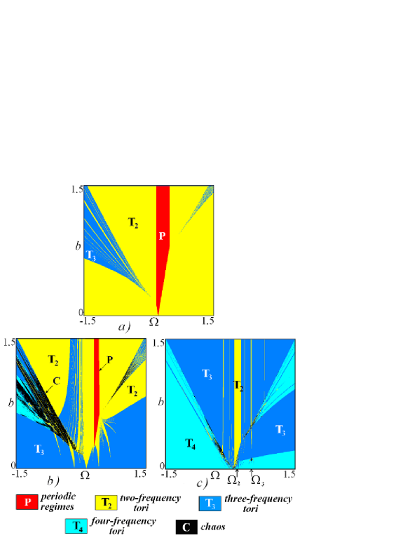
Figure 2: Charts of Lyapunov exponents for the model systems of two (a) and three (b and c) driven oscillators. Parameter values are $\Delta_{1}=0.3$, $\Delta_{2}=1$, $\mu=0.4$ (a), $\mu=0.4$ (b), $\mu=015$ (c). The color coding is indicated in the bottom part of the figure. The marks $\Omega_{2}$ and $\Omega_{3}$ indicate frequencies of the second and the third oscillators respectively.

One can see that the domain of complete locking of all oscillators by the external driving force $P$ decreases notably in width. Besides, a finite amplitude threshold of the complete synchronization appears.

The regions of three-frequency tori disappear, and instead of them the four-frequency tori and chaos arise. Besides, a finite amplitude threshold of the complete synchronization appears. At small amplitude three-frequency tori replace the two-frequency quasiperiodicity.

It is interesting to discuss the picture in the context of the Ruelle – Takens hypothesis. Adding the third oscillator obviously facilitates destruction of the three-frequency tori, but it can result in appearance either of chaos, or of the four-frequency tori. The domains of occurrence of these types of attractors coexist on the parameter plane. Both quasiperiodicity and chaos look typical, no one prevails. So, we do not observe an extrusion of the tori by the chaotic regimes, as one could expect, perhaps, basing on the Ruelle – Takens assertions.

The winding-number chart of two-frequency tori shown in Fig.3 demonstrates the complexity of the observed picture.

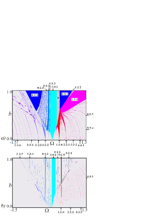
Figure 3: A chart of two-frequency tori for the system (5). Parameters are corresponded to Figs.1b and c.

In terms of phase equations (5), a two-frequency torus corresponds to a closed invariant curve in the phase box ($\psi_{1}$, $\psi_{2}$, $\psi_{3}$), with boundaries (0, 2$\pi$). The parameter scan in Fig.3 is obtained as follows. For each parameter value we determine via numerical simulations a set of numbers $p$, $q$, $r$, which are essentially the numbers of intersections of the invariant curve with the edge surfaces of the phase box (with exclusion of returns). These numbers determine what we call the winding number of the invariant curve: $w=p:q:r$. Then, each point is attributed with a definite color depending on the winding number we got. The light gray tone designates regimes, which do not have a definite quantifier in the frame of the procedure, like the three-frequency tori, four-frequency tori, or chaos. The domains of main resonances are marked with subscriptions in the respective areas of the chart in Fig.3. Note that the regimes of type $w=0:q:r$ correspond to partial locking of the first oscillator by the external force, and the regime $w=1:1:1$ corresponds to synchronization of all oscillators as the unified system.

Now let us consider transformation of the picture under decrease of the coupling between the oscillators up to the value $\mu=0.15$. The respective diagram is shown in Fig.2c. In this case, the four-frequency tori dominate, and they effectively extrude the chaotic regimes, which occupy now only some extremely narrow strip-like areas placed mainly along the borders of three-frequency tori domains. The four-frequency tori dominate as well at small amplitudes, so, the amplitude threshold for them vanishes. Additionally, there is a small chaotic region in a neighborhood of the frequency of the third oscillator, which has, however, a non-zero amplitude threshold.

A characteristic feature of the Fig.2c is disappearance of the regime of the complete synchronization $P$. Instead, a narrow strip of the two-frequency tori remains. The winding-number chart for this case shown in Fig.3b illustrates this effect. One can see the regimes with winding number $w=0:0:1$ instead of the region of complete synchronization. This regime corresponds to partial locking of the first and second oscillator by the external force. This phase of the third oscillator demonstrates unlimited growth. Thus the system of three oscillators can be configured so that complete synchronization is impossible. This is important difference from the case of two oscillators.

In this paper we have considered the chain of three oscillators with external force effecting the outermost one. Otherwise, there are many possibilities for coupling and forcing: we may take the ring of oscillators or affect the oscillators simultaneously, etc. It may be conjectured that 4D-tori would persist for either configuration, but what concerns the possibility of absence of complete synchronization, the answer may depend on concrete configuration of coupling and external forcing.

5 CONCLUSION

A passage from two-mode to three-mode self-oscillatory system driven by periodic external signal gives rise to destruction of three-frequency tori with formation of regions of four-frequency tori and chaos. At moderate coupling parameter values neither of these regimes dominates. Decrease of coupling leads to almost complete extrusion of chaos by the four-frequency quasiperiodic regimes. Besides, such regimes dominate at small amplitudes of external driving. New effects for the case of three oscillators is that at sufficiently small coupling the regime of the complete synchronization of three oscillators by the external driving disappear.

The work has been supported by RFBR, grant No 09-02-00426.

References

- [1] A. Pikovsky, M. Rosenblum, J. Kurths, Synchronization: A Universal Concept in Nonlinear Science (Cambridge University Press, Cambridge, England, 2001).
- [2] J. Guckenheimer, P,Holmes, Nonlinear oscillations, dynamical systems, and bifurcations of vector fields (Springer, New York, 1983); I. I. Blekhman, Synchronization in Science and Technology (ASME Press, New York, 1988); Y. Kuramoto, Chemical Oscillations, Waves, and Turbulence (Springer-Verlag, New York. 1984); L Glass, M.C. MacKey, From Clocks to Chaos (Princeton University Press, 1988); A. Winfree, The Geometry of Biological Time, 2nd. ed. (Springer-Verlag, New York, 2001).
- [3] L.D. Landau, Doklady Akademii Nauk SSSR, 44, 1944, 339 (1944) (In Russian); E. Hopf, Communications on Pure and Applied Mathematics, 1 303 (1948).
- [4] D. Ruelle, F Takens, Commun Math Phys, 20, 167 (1971).
- [5] V. Anishchenko, S. Astakhov, T. Vadivasova, Europhysics Letters, 86, 30003 (2009); G.B. Ermentrout and N. Kopell, I SIAM J. Math. Anal., 15 215 (1984); G.B. Ermentrout, J. Math. Biol. 23 55 (1985); Kopell N. and Ermentrout G.B., Comm. Pure Appl. Math. 39 623 (1986); Aronson D.G., Rementrout G.B. and Kopell N., PhysicaD 41 403 (1990).
- [6] A. Kuznetsov, N. Stankevich. L. Turukina, Physica D 238, 1203, 2009.
- [7] M Ivanchenko, G. Osipov, V. Shalfeev, J. Kurths, Physica D 189, 8 (2004).