Stochastic Optimal Multi-Modes Switching with a
Viscosity Solution Approach

Abstract

We consider the problem of optimal multi-modes switching in finite horizon, when the state of the system, including the switching cost functions are arbitrary ($g_{ij}(t,x)\geq 0$). We show existence of the optimal strategy, and give when the optimal strategy is finite via a verification theorem. Finally, when the state of the system is a markov process, we show that the vector of value functions of the optimal problem is the unique viscosity solution to the system of $m$ variational partial differential inequalities with inter-connected obstacles.

$\mathbf{Keywords}$. Real options, Backward stochastic differential equations, Snell envelope, Stopping times, Switching, Viscosity solution of PDEs, Variational inequalities

AMS Classification subjects. 60G40, 62P20, 91B99, 91B28, 35B37, 49L25

1 Introduction

We consider a power plant which produces electricity and which has several modes of production, e.g., the lower, the middle and the intensive modes. The price $(X_{t})_{t\geq 0}$ of electricity in the market fluctuates in reaction to many factors such as demand level, weather conditions, unexpected outages etc. Moreover, electricity is non-storable once produced, it should be almost immediately consumed. Therefore, as a consequence, the station produces electricity in its instantaneous most profitable mode known that when the plant is in mode $i\in\mathcal{I}$, the yield per unit time $dt$ is given by means of $\psi_{i}(t,X_{t})dt$ and, on the other hand, switching the plant from the mode $i$ to the mode $j$ is not free and generates expenditures given by $g_{ij}(t,X_{t})$ and possibly by other factors in the energy market.

The switching from one regime to another one is realized sequentially at random times which are part of the decisions. So the manager of the power plant faces two main issues:

$(i)$ when should she decide to switch the production from its current mode to another one?

$(ii)$ to which mode the production has to be switched when the decision of switching is made?

The manager faces the issue of finding the optimal strategy of management of the plant. This is related with the price of the power plant in the energy market.

Optimal switching problems for stochastic systems were studied by several authors (see e.g. [2, 3, 5, 10, 11, 12, 14, 15, 16, 20, 28, 31] and the references therein). The motivations are mainly related to decision making in the economic sphere. In order to tackle those problems, authors use mainly two approaches. Either a probabilistic one [11, 12, 20] or an approach which uses partial differential inequalities (PDIs for short) [2, 5, 14, 16, 31, 28].

In the finite horizon framework Djehiche et al. [12] have studied the multi-modes switching problem in using probabilistic tools. They have proved existence of a solution and found an optimal strategy when the switching costs from state $i$ to state $j$ is strictly non–negative ($g_{ij}>\alpha>0$). The partial differential equation approach of this work has been carried out by El Asri and Hamadène [16]. We showed that when the price process $(X_{t}:t\geq 0)$ is solution of a Markovian stochastic differential equation, then this problem is associated to a system of variational inequalities with interconnected obstacles for which we provided a solution in viscosity sense. This solution is bind to the value function of the problem. Moreover the solution of the system is unique.

Using purely probabilistic tools such as the system of backward stochastic differential equations with oblique reflections (RBSDEs for short), Hamadène and Zhang [21] have considered this optimal switching problem when the switching costs from state $i$ to state $j$ is non–negative $g_{ij}$. But in general case the optimal strategy may not exist.

The purpose of this work is to fill in this gap by providing a solution to the optimal multiple switching problem using probabilistic tools and partial differential equation approach.

We prove existence and provide a characterization of an optimal strategy of this problem when the payoff rates $\psi_{i}$ and the switching costs $g_{ij}\geq 0$ are adapted only to the filtration generated by a Brownian motion. Later on, in the case when $X$ is a solution of a SDE, we show that the value function of the problem is associated an uplet of deterministic functions $(v^{1},\dots,v^{m})$ which is the unique solution of the following system of PDIs:

(1.1) $$\left\{\begin{array}[]{l}\min\left\{v_{i}(t,x)-\max\limits_{j\in\mathcal{I}^{-i}}\left\{-g_{ij}(t,x)+v_{j}(t,x)\right\},-\partial_{t}v_{i}(t,x)-\mathcal{A}v_{i}(t,x)-\psi_{i}(t,x)\right\}=0\\ \forall\,\,(t,x)\in[0,T]\times\mathbb{R}^{k},\,\,i\in\mathcal{I}=\{1,...,m\},\text{\thinspace\ and \thinspace\ }v_{i}(T,x)=0,\end{array}\right.$$

where $\mathcal{A}$ an operator associated with a diffusion process and $\mathcal{I}^{-i}:=\mathcal{I}\setminus\{i\}$. It turns out that this system is the deterministic version of the Verification Theorem of the optimal multi-modes switching problem in infinite horizon.

This paper is organized as follows: In Section 2, we formulate the problem and give the related definitions. In Section 3, we shall introduce the optimal switching problem under consideration and give its probabilistic Verification Theorem. It is expressed by means of a Snell envelope. Then we introduce the approximating scheme which enables us to construct a solution for the Verification Theorem. Moreover we give some properties of that solution, especially the dynamic programming principle. Section 4 is devoted to the connection between the optimal switching problem, the Verification Theorem and the associated system of PDIs. This connection is made through BSDEs with one reflecting obstacle in the Markovian case. Further we provide some estimate for the optimal strategy of the switching problem which, in combination with the dynamic programming principle, plays a crucial role in the proof of existence of a solution for (1.1). In Section 5, we show that the solution of PDIs is unique in the class of continuous functions which satisfy a polynomial growth condition. In section 6 some numerical examples are given. We close this paper an appendix in which some technical results are proved.

2 Assumptions and formulation of the problem

Throughout this paper $T$ (resp. $k,\,d$) is a fixed real (resp. integers) positive numbers.
Let

$(i)$ $b:[0,T]\times\mathbb{R}^{k}\rightarrow\mathbb{R}^{k}$ and $\sigma:[0,T]\times\mathbb{R}^{k}\rightarrow\mathbb{R}^{k\times d}$ be two continuous functions for which there exists a constant $C>0$ such that for any $t\in[0,T]$ and $x,x^{\prime}\in\mathbb{R}^{k}$

(2.1) $$|\sigma(t,x)-\sigma(t,x^{\prime})|+|b(t,x)-b(t,x^{\prime})|\leq C|x-x^{\prime}|,$$

$(ii)$ for $i,j\in\mathcal{I}=\{1,\ldots,m\}$, $g_{ij}:[0,T]\times\mathbb{R}^{k}\rightarrow\mathbb{R}$ and $\psi_{i}:[0,T]\times\mathbb{R}^{k}\rightarrow\mathbb{R}$ are continuous functions and of polynomial growth, $i.e.$ there exist some positive constants $C$ and $\gamma$ such that for each $i,j\in\mathcal{I}$:

(2.2) $$|\psi_{i}(t,x)|+|g_{ij}(t,x)|\leq C(1+|x|^{\gamma}),\,\,\forall\;(t,x)\in[0,T]\times\mathbb{R}^{k},$$

$(iii)$ for any $(t,x)\in[0,T]\times\mathbb{R}^{k}$, $g_{ij}(t,x)$ are satisfying

(2.3) $$g_{ii}(t,x)=0,\quad g_{ij}(t,x)\geq 0\quad\mbox{and}\quad g_{ij}(t,x)+g_{jk}(t,x)>g_{ik}(t,x),\quad j\neq i,\ k\in\mathcal{I},$$

which means that it is less expensive to switch directly in one step from regime $i$ to $k$ than in two steps via an intermediate regime $j$.

Moreover we assume that there exists a constant $\alpha>0$ such that for any $(t,x)\in[0,T]\times\mathbb{R}^{k}$,

(2.4) $$g_{ij}(t,x)+g_{ji}(t,x)>\alpha,\qquad i\neq j\in\mathcal{I}.$$

This condition means that switching back and forth is not free.

We now consider the following system of $m$ variational inequalities with inter-connected obstacles: $\forall\,\,i\in\mathcal{I}$

(2.5) $$\left\{\begin{array}[]{l}\min\left\{v_{i}(t,x)-\max\limits_{j\in\mathcal{I}^{-i}}\left\{-g_{ij}(t,x)+v_{j}(t,x)\right\},-\partial_{t}v_{i}(t,x)-\mathcal{A}v_{i}(t,x)-\psi_{i}(t,x)\right\}=0,\\ v_{i}(T,x)=0,\end{array}\right.$$

where $\mathcal{A}$ is given by:

(2.6) $$\mathcal{A}=\frac{1}{2}\sum_{i,j=1}^{m}(\sigma\sigma^{\ast})_{ij}(t,x)\frac{\partial^{2}}{\partial x_{i}\partial x_{j}}+\sum_{i=1}^{m}b_{i}(t,x)\frac{\partial}{\partial x_{i}}\,;$$

hereafter the superscript $(^{\ast})$ stands for the transpose, $Tr$ is the trace operator and finally $\left\langle x,y\right\rangle$ is the inner product of $x,y\in\mathbb{R}^{k}$.

The main objective of this paper is to focus on the uniqueness of the solution in viscosity sense of (2.5) whose definition is:

Definition 2.1

Let $(v_{1},\ldots,v_{m})$ be a $m$-uplet of continuous functions defined on $[0,T]\times\mathbb{R}^{k}$, $\mathbb{R}$-valued and such that $v_{i}(T,x)=0$ for any $x\in\mathbb{R}^{k}$ and $i\in\mathcal{I}$. The $m$-uplet $(v_{1},\ldots,v_{m})$ is called:

• a viscosity supersolution (resp. subsolution) of the system (2.5) if for each fixed $i\in\mathcal{I}$, for any $(t_{0},x_{0})\in[0,T]\times\mathbb{R}^{k}$ and any function $\varphi_{i}\in\mathcal{C}^{1,2}([0,T]\times\mathbb{R}^{k})$ such that $\varphi_{i}(t_{0},x_{0})=v_{i}(t_{0},x_{0})$ and $(t_{0},x_{0})$ is a local maximum of $\varphi_{i}-v_{i}$ (resp. minimum), we have:

  (2.7) $$\min\left\{v_{i}(t_{0},x_{0})-\max\limits_{j\in\mathcal{I}^{-i}}\left\{-g_{ij}(t_{0},x_{0})+v_{j}(t_{0},x_{0})\right\},-\partial_{t}\varphi_{i}(t_{0},x_{0})-\mathcal{A}\varphi_{i}(t_{0},x_{0})-\psi_{i}(t_{0},x_{0})\right\}\geq 0\,\,(\mbox{resp.}\leq 0).$$

• a viscosity solution if it is both a viscosity supersolution and subsolution. $\Box$

There is an equivalent formulation of this definition (see e.g. [6]) which we give because it will be useful later. So firstly we define the notions of superjet and subjet of a continuous function $v$.

Definition 2.2

Let $v\in\mathcal{C}((0,T)\times\mathbb{R}^{k})$, $(t,x)$ an element of $(0,T)\times\mathbb{R}^{k}$ and finally $\mathbb{S}_{k}$ the set of $k\times k$ symmetric matrices. We denote by $J^{2,+}v(t,x)$ (resp. $J^{2,-}v(t,x)$), the superjets (resp. the subjets) of $v$ at $(t,x)$, the set of triples $(p,q,X)\in\mathbb{R}\times\mathbb{R}^{k}\times\mathbb{S}_{k}$ such that:

$$v(s,y) \leq v(t,x)+p(s-t)+\langle q,y-x\rangle+\frac{1}{2}\langle X(y-x),y-x\rangle+o(|s-t|+|y-x|^{2})$$

$$(resp.\quad v(s,y) \geq v(t,x)+p(s-t)+\langle q,y-x\rangle+\frac{1}{2}\langle X(y-x),y-x\rangle+o(|s-t|+|y-x|^{2})).$$

Note that if $\varphi-v$ has a local maximum (resp. minimum) at $(t,x)$, then we obviously have:

$$\left(D_{t}\varphi(t,x),D_{x}\varphi(t,x),D_{xx}^{2}\varphi(t,x)\right)\in J^{2,-}v(t,x)\,\,\,(\mbox{resp. }J^{2,+}v(t,x)).\Box$$

We now give an equivalent definition of a viscosity solution of the parabolic system with inter-connected obstacles (2.5).

Definition 2.3

Let $(v_{1},\ldots,v_{m})$ be a $m$-uplet of continuous functions defined on $[0,T]\times\mathbb{R}^{k}$, $\mathbb{R}$-valued and such that $(v_{1},\ldots,v_{m})(T,x)=0$ for any $x\in\mathbb{R}^{k}$. The $m$-uplet $(v_{1},\ldots,v_{m})$ is called a viscosity supersolution (resp. subsolution) of (2.5) if for any $i\in\mathcal{I}$, $(t,x)\in(0,T)\times\mathbb{R}^{k}$ and $(p,q,X)\in J^{2,-}v_{i}(t,x)$ (resp. $J^{2,+}v_{i}(t,x)$),

$$min\left\{v_{i}(t,x)-\max\limits_{j\in\mathcal{\ I}^{-i}}(-g_{ij}(t,x)+v_{j}(t,x)),-p-\frac{1}{2}Tr[\sigma^{*}X\sigma]-\langle b,q\rangle-\psi_{i}(t,x)\right\}\geq 0\,\,(resp.\leq 0).$$

It is called a viscosity solution it is both a viscosity subsolution and supersolution. $\Box$

As pointed out previously we will show that system (2.5) has a unique solution in viscosity sense. This system is the deterministic version of the optimal $m$-states switching problem will describe briefly in the next section.

3 The optimal $m$-states switching problem

3.1 Setting of the problem

Let $(\Omega,\mathcal{F},P)$ be a fixed probability space on which is defined a standard $d$-dimensional Brownian motion $B=(B_{t})_{0\leq t\leq T}$ whose natural filtration is $(\mathcal{F}_{t}^{0}:=\sigma\{B_{s},s\leq t\})_{0\leq t\leq T}$. Let $\mathbf{F}=(\mathcal{F}_{t})_{0\leq t\leq T}$ be the completed filtration of $(\mathcal{F}_{t}^{0})_{0\leq t\leq T}$ with the $P$-null sets of $\mathcal{F}$.
Let:

- $\mathcal{P}$ be the $\sigma$-algebra on $[0,T]\times\Omega$ of $\mathbf{F}$-progressively measurable sets;

- $\mathcal{M}^{2,k}$ be the set of $\mathcal{P}$-measurable and $\mathbb{R}^{k}$-valued processes $w=(w_{t})_{t\leq T}$ such that $E[\int_{0}^{T}|w_{s}|^{2}ds]<\infty$ and $\mathcal{S}^{2}$ be the set of $\mathcal{P}$-measurable, continuous processes ${w}=({w}_{t})_{t\leq T}$ such that $E[\sup_{t\leq T}|{w}_{t}|^{2}]<\infty$;

- for any stopping time $\tau\in[0,T]$, $\mathcal{T}_{\tau}$ denotes the set of all stopping times $\theta$ such that $\tau\leq\theta\leq T$.

Let $\mathcal{I}$ be the set of all possible activity modes of the production of a power plant. A management strategy of the plant consists, on the one hand, of the choice of a sequence of nondecreasing stopping times $(\tau_{n})_{n\geq 1}$ (i.e. $\tau_{n}\leq\tau_{n+1}$ and $\tau_{0}=0$) where the manager decides to switch the activity from its current mode to another one. On the other hand, it consists of the choice of the mode $\xi_{n}$, which is an $\mathcal{F}_{\tau_{n}}$-measurable random variable taking values in $\mathcal{I}$, to which the production is switched at $\tau_{n}$ from its current mode. Therefore the admissible management strategies of the plant are the pairs $(\delta,\xi):=((\tau_{n})_{n\geq 1},(\xi_{n})_{n\geq 1})$ and the set of these strategies is denoted by $\mathcal{D}$.

Let $X:=(X_{t})_{0\leq t\leq T}$ be an $\mathcal{P}$-measurable, $\mathbb{R}^{k}$-valued continuous stochastic process which stands for the market price of $k$ factors which determine the market price of the commodity. Assuming that the production activity is in mode 1 at the initial time $t=0$, let $(u_{t})_{t\leq T}$ denote the indicator of the production activity’s mode at time $t\in[0,T]$ :

(3.1) $$u_{t}=\mathbf{1}_{[0,\tau_{1}]}(t)+\sum_{n\geq 1}\xi_{n}\mathbf{1}_{(\tau_{n},\tau_{n+1}]}(t).$$

Then for any $t\leq T$, the state of the whole economic system related to the project at time $t$ is represented by the vector:

(3.2) $$(t,X_{t},u_{t})\in[0,T]\times\mathbb{R}^{k}\times\mathcal{I}.$$

Finally, let $\psi_{i}(t,X_{t})$ be the instantaneous profit when the system is in state $(t,X_{t},i)$, and for $i,j\in\mathcal{I}$ $\ i\neq j$, let $g_{ij}(t,X_{t})$ denote the switching cost of the production at time $t$ from current mode $i$ to another mode $j$. Then if the plant is run under the strategy $(\delta,\xi)=((\tau_{n})_{n\geq 1},(\xi_{n})_{n\geq 1})$ the expected total profit is given by:

$$J(\delta,\xi)=E\left[\int_{0}^{T}\psi_{u_{s}}(s,X_{s})ds-\sum_{n\geq 1}g_{u_{\tau_{n-1}}u_{\tau_{n}}}(\tau_{n},X_{\tau_{n}})\mathbf{1}_{[\tau_{n}<T]}\right].$$

Therefore the problem we are interested in is to find an optimal strategy $i.e.$ a strategy $(\delta^{\ast},\xi^{\ast})$ such that $J(\delta^{\ast},\xi^{\ast})\geq J(\delta,\xi)$ for any $(\delta,\xi)\in\mathcal{D}$.

Note that in order that the quantity $J(\delta,\xi)$ makes sense, we assume throughout this paper that, for any $i,j\in\mathcal{I}$ the processes $(\psi_{i}(t,X_{t}))_{t\leq T}$ and $(g_{ij}(t,X_{t}))_{t\leq T}$ belong to $\mathcal{M}^{2,1}$ and $\mathcal{S}^{2}$ respectively. There is one to one correspondence between the pairs $(\delta,\xi)$ and the pairs $(\delta,u)$. Therefore throughout this paper one refers indifferently to $(\delta,\xi)$ or $(\delta,u)$.

3.2 The Verification Theorem

To tackle the problem described above Djehiche et al. [12] have introduced a Verification Theorem which is expressed by means of Snell envelope of processes. The Snell envelope of a stochastic process $(\eta_{t})_{t\leq T}$ of $\mathcal{S}^{2}$ (with a possible positive jump at $T$) is the lowest supermartingale $R(\eta):=(R(\eta)_{t})_{t\leq T}$ of $\mathcal{S}^{2}$ such that for any $t\leq T$, $R(\eta)_{t}\geq\eta_{t}$. It has the following expression:

$$\forall\;t\leq T,\ R(\eta)_{t}=\mathop{\mathrm{e}sssup}_{\tau\in\mathcal{T}_{t}}E[\eta_{\tau}|\mathcal{F}_{t}]\mbox{ and satisfies }R(\eta)_{T}=\eta_{T}.$$

For more details owe refer to [4, 17, 19].

The Verification Theorem for the $m$-states optimal switching problem is the following:

Theorem 3.1

Assume that there exist $m$ processes $(Y^{i}:=(Y_{t}^{i})_{0\leq t\leq T},i=1,\ldots,m)$ of $\mathcal{S}^{2}$ such that:

(3.3) $$\forall\;t\leq T,\,\,Y_{t}^{i}=\mathop{\mathrm{e}sssup}_{\tau\geq t}E\left[\int_{t}^{{\tau}}\psi_{i}(s,X_{s})ds+\max\limits_{j\in\mathcal{I}^{-i}}(-g_{ij}(\tau,X_{\tau})+Y_{\tau}^{j})\mathbf{1}_{[\tau<T]}|\mathcal{F}_{t}\right],\;Y_{T}^{i}=0.$$

Then:

• $Y_{0}^{1}=\sup\limits_{(\delta,\xi)\in\mathcal{D}}J(\delta,u).$

• Define the sequence of $\mathbf{F}$-stopping times $\delta^{\ast}=(\tau_{n}^{\ast})_{n\geq 1}$ as follows :

  $$\begin{array}[]{lll}\tau_{1}^{\ast}&=&\inf\left\{s\geq 0,\quad Y_{s}^{1}=\max\limits_{j\in{\mathcal{\ I}^{-1}}}(-g_{1j}(s,X_{s})+Y_{s}^{j})\right\}\wedge T,\\ \tau_{n}^{\ast}&=&\inf\left\{s\geq\tau_{n-1}^{\ast},\quad Y_{s}^{u_{\tau_{n-1}^{\ast}}}=\max\limits_{k\in\mathcal{I}\backslash\{u_{\tau_{n-1}^{\ast}}\}}(-g_{u_{\tau_{n-1}^{\ast}}k}(s,X_{s})+Y_{s}^{k})\right\}\wedge T,\quad\mbox{for}\quad n\geq 2,\end{array}$$

  where:

  • $u_{\tau_{1}^{\ast}}=\sum\limits_{j\in\mathcal{\ I}}j\mathbf{1}_{\{\max\limits_{k\in\mathcal{\ I}^{-1}}(-g_{1k}(\tau_{1}^{\ast},X_{\tau_{1}^{\ast}})+Y_{\tau_{1}^{\ast}}^{k})=-g_{1j}(\tau_{1}^{\ast},X_{\tau_{1}^{\ast}})+Y_{\tau_{1}^{\ast}}^{j}\}};$

  • for any $n\geq 1$ and $t\geq\tau_{n}^{\ast},$ $Y_{t}^{u_{\tau_{n}^{\ast}}}=\sum\limits_{j\in\mathcal{I}}\mathbf{1}_{[u_{\tau_{n}^{\ast}}=j]}Y_{t}^{j}$

  • for any $n\geq 2,\,\,u_{\tau_{n}^{\ast}}=l$ on the set

    $$\left\{\max\limits_{k\in\mathcal{I}\backslash\{{u_{\tau_{n-1}^{\ast}}}\}}(-g_{u_{\tau_{n-1}^{\ast}}k}(\tau_{n}^{\ast},X_{\tau_{n}^{\ast}})+Y_{\tau_{n}^{\ast}}^{k})=-g_{u_{\tau_{n-1}^{\ast}l}}(\tau_{n}^{\ast},X_{\tau_{n}^{\ast}})+Y_{\tau_{n}^{\ast}}^{l}\right\}$$

    with $g_{u_{\tau_{n-1}^{\ast}k}}(\tau_{n}^{\ast},X_{\tau_{n}^{\ast}})=\sum\limits_{j\in\mathcal{I}}\mathbf{1}_{[u_{\tau_{n-1}^{\ast}}=j]}g_{jk}(\tau_{n}^{\ast},X_{\tau_{n}^{\ast}})$ and $\mathcal{I}\backslash\{u_{\tau_{n-1}^{\ast}}\}=\sum\limits_{j\in\mathcal{I}}\mathbf{1}_{[u_{\tau_{n-1}^{\ast}}=j]}\mathcal{I}^{-j}$.
    Then the strategy $(\delta^{\ast},u^{\ast})$ satisfies

    $$E\left[\sum_{k\geq 1}g_{u_{\tau_{k-1}^{\ast}}u_{\tau_{k}^{\ast}}}({\tau_{k}^{\ast}},X_{{\tau_{k}^{\ast}}})\mathbf{1}_{[\tau_{k}^{\ast}<T]}\right]<+\infty$$

    and it is optimal.

  • If

    $$E\left[\sum\limits_{k\geq 1}g_{u_{\tau_{k}^{\ast}}u_{\tau_{k-1}^{\ast}}}({\tau_{k}^{\ast}},X_{{\tau_{k}^{\ast}}})\mathbf{1}_{[\tau_{k}^{\ast}<T]}\right]<+\infty$$

    or $g_{ij}$ is constant, then the optimal strategy $(\delta^{\ast},u^{\ast})$ is finite.

$Proof.$ The proof is divided in four steps
Step 1. (i) It consists in showing that for any $t\leq T,$ $Y_{t}^{i}$, as defined by (3.3), is the expected total profit or the value function of the optimal problem, given that the system is in mode $i$ at time $t$. More precisely,

$$Y_{t}^{i}=\mathop{\mathrm{e}sssup}_{(\delta,u)\in\mathcal{D}_{t}}E\left[\int_{t}^{T}\psi_{i}(s,X_{s})ds-\sum_{k\geq 1}g_{u_{\tau_{k-1}}u_{\tau_{k}}}(\tau_{k},X_{{\tau_{k}}})\mathbf{1}_{[\tau_{k}<T]}|\mathcal{F}_{t}\right],$$

where $\mathcal{D}_{t}$ is the set of strategies such that $\tau_{1}\geq t$, $P$-a.s. if at time $t$ the system is in the mode $i$.

Let us admit for a moment the following Lemma whose proof is given in the appendix.

Lemma 3.1

For every $\tau_{1}^{\ast}\leq t\leq T$.

(3.4) $$Y_{t}^{u_{\tau_{1}^{\ast}}}=\mathop{\mathrm{e}sssup}_{\tau\geq t}E\left[\int_{t}^{\tau}\psi_{u_{\tau_{1}^{\ast}}}(s,X_{s})ds+\max\limits_{j\in\mathcal{I}^{-u_{\tau_{1}^{\ast}}}}(-g_{u_{\tau_{1}^{\ast}}j}(\tau,X_{\tau})+Y_{\tau}^{j})\mathbf{1}_{[\tau<T]}|\mathcal{F}_{t}\right].\;\Box$$

From properties of the Snell envelope and at time $t=0$ the system is in mode $1$, we have:

$$Y_{0}^{1} = E\left[\int_{0}^{\tau_{1}^{\ast}}\psi_{1}(s,X_{s})ds+\max\limits_{j\in\mathcal{I}^{-1}}(-g_{1j}({\tau_{1}^{\ast}},X_{\tau_{1}^{\ast}})+Y_{\tau_{1}^{\ast}}^{j})\mathbf{1}_{[\tau_{1}^{\ast}<T]}\right]$$

$$= E\left[\int_{0}^{\tau_{1}^{\ast}}\psi_{1}(s,X_{s})ds+(-g_{1u_{\tau_{1}^{\ast}}}({\tau_{1}^{\ast}},X_{\tau_{1}^{\ast}})+Y_{\tau_{1}^{\ast}}^{u_{\tau_{1}^{\ast}}})\mathbf{1}_{[\tau_{1}^{\ast}<T]}\right].$$

Now, from Lemma 3.1 and the definition of $\tau_{2}^{\ast}$ we have:

$$Y_{\tau_{1}^{\ast}}^{u_{\tau_{1}^{\ast}}} = E\left[\int_{\tau_{1}^{\ast}}^{\tau_{2}^{\ast}}\psi_{u_{\tau_{1}^{\ast}}}(s,X_{s})ds+\max\limits_{j\in\mathcal{I}^{-u_{\tau_{1}^{\ast}}}}(-g_{u_{\tau_{1}^{\ast}}j}(\tau_{2}^{\ast},X_{\tau_{2}^{\ast}})+Y_{\tau_{2}^{\ast}}^{j})\mathbf{1}_{[\tau_{2}^{\ast}<T]}|\mathcal{F}_{\tau_{1}^{\ast}}\right]$$

$$= E\left[\int_{\tau_{1}^{\ast}}^{\tau_{2}^{\ast}}\psi_{u_{\tau_{1}^{\ast}}}(s,X_{s})ds+(-g_{u_{\tau_{1}^{\ast}}u_{\tau_{2}^{\ast}}}(\tau_{2}^{\ast},X_{\tau_{2}^{\ast}})+Y_{\tau_{2}^{\ast}}^{u_{\tau_{2}^{\ast}}})\mathbf{1}_{[\tau_{2}^{\ast}<T]}|\mathcal{F}_{\tau_{1}^{\ast}}\right].$$

It implies that

$$Y_{0}^{1} = E\left[\int_{0}^{\tau_{1}^{\ast}}\psi_{1}(s,X_{s})ds-g_{1u_{\tau_{1}^{\ast}}}({\tau_{1}^{\ast}},X_{\tau_{1}^{\ast}})\mathbf{1}_{[\tau_{1}^{\ast}<T]}\right]$$

$$+E\left[\int_{\tau_{1}^{\ast}}^{\tau_{2}^{\ast}}\psi_{u_{\tau_{1}^{\ast}}}(s,X_{s})ds+(-g_{u_{\tau_{1}^{\ast}}u_{\tau_{2}^{\ast}}}({\tau_{2}^{\ast}},X_{\tau_{2}^{\ast}})+Y_{\tau_{2}^{\ast}}^{u_{\tau_{2}^{\ast}}})\mathbf{1}_{[\tau_{2}^{\ast}<T]}|\mathcal{F}_{\tau_{1}^{\ast}}\right]$$

$$= E\left[\int_{0}^{\tau_{1}^{\ast}}\psi_{1}(s,X_{s})ds+\int_{\tau_{1}^{\ast}}^{\tau_{2}^{\ast}}\psi_{u_{\tau_{1}^{\ast}}}(s,X_{s})ds\right.$$

$$\left.-g_{1u_{\tau_{1}^{\ast}}}({\tau_{1}^{\ast}},X_{\tau_{1}^{\ast}})\mathbf{1}_{[\tau_{1}^{\ast}<T]}-g_{u_{\tau_{1}^{\ast}}u_{\tau_{2}^{\ast}}}({\tau_{2}^{\ast}},X_{\tau_{2}^{\ast}})\mathbf{1}_{[\tau_{2}^{\ast}<T]}+Y_{\tau_{2}^{\ast}}^{u_{\tau_{2}^{\ast}}}\mathbf{1}_{[\tau_{2}^{\ast}<T]}\right],$$

since $[\tau_{2}^{\ast}<T]\subset[\tau_{1}^{\ast}<T]$. Therefore

(3.5) $$Y_{0}^{1}=E\left[\int_{0}^{\tau_{2}^{\ast}}\psi(s,X_{s},u_{s})ds-g_{1u_{\tau_{1}^{\ast}}}({\tau_{1}^{\ast}},X_{\tau_{1}^{\ast}})\mathbf{1}_{[\tau_{1}^{\ast}<T]}-g_{u_{\tau_{1}^{\ast}}u_{\tau_{2}^{\ast}}}({\tau_{2}^{\ast}},X_{\tau_{2}^{\ast}})\mathbf{1}_{[\tau_{2}^{\ast}<T]}+Y_{\tau_{2}^{\ast}}^{u_{\tau_{2}^{\ast}}}\mathbf{1}_{[\tau_{2}^{\ast}<T]}\right],$$

since between $0$ and $\tau_{1}^{\ast}$ (resp. $\tau_{1}^{\ast}$ and $\tau_{2}^{\ast}$) the production is in regime $1$ (resp. regime $u_{\tau_{1}^{\ast}}$) and then $u_{t}=1$ (resp. $u_{t}=u_{\tau_{1}^{\ast}}$) which implies that

$$\int_{0}^{\tau_{2}^{\ast}}\psi(s,X_{s},u_{s})ds=\int_{0}^{\tau_{1}^{\ast}}\psi_{1}(s,X_{s})ds+\int_{\tau_{1}^{\ast}}^{\tau_{2}^{\ast}}\psi_{u_{\tau_{1}^{\ast}}}(s,X_{s})ds.$$

Repeating this reasoning as many times as necessary we obtain that for any $n\geq 0,$

$$Y_{0}^{1}=E\left[\int_{0}^{\tau_{n}^{\ast}}\psi(s,X_{s},u_{s})ds-\sum_{k=1}^{n}g_{u_{\tau_{k-1}^{\ast}}u_{\tau_{k}^{\ast}}}({\tau_{k}^{\ast}},X_{{\tau_{k}^{\ast}}})\mathbf{1}_{[\tau_{k}^{\ast}<T]}+Y_{\tau_{n}^{\ast}}^{u_{\tau_{n}^{\ast}}}\mathbf{1}_{[\tau_{n}^{\ast}<T]}\right].$$

Then, the strategy $(\delta^{\ast},u^{\ast})$ satisfies

$$E\left[\sum\limits_{k\geq 1}g_{u_{\tau_{k-1}^{\ast}}u_{\tau_{k}^{\ast}}}({\tau_{k}^{\ast}},X_{{\tau_{k}^{\ast}}})\mathbf{1}_{[\tau_{k}^{\ast}<T]}\right]<+\infty.$$

If not $Y_{0}^{1}=-\infty$ which contradicts the assumption $Y^{i}\in\mathcal{S}^{2}$. Therefore, taking the limit as $n\rightarrow+\infty$ we obtain $Y_{0}^{1}=J(\delta^{\ast},u^{\ast})$.
Step 2. (ii) We show that the strategy $(\delta^{\ast},u^{\ast})$ it is optimal i.e. $J(\delta^{\ast},u^{\ast})\geq J(\delta,u)$ for any $(\delta,u)\in\mathcal{D}$.
The definition of the Snell envelope yields

$$Y_{0}^{1} \geq E\left[\int_{0}^{\tau_{1}}\psi_{1}(s,X_{s})ds+\max\limits_{j\in\mathcal{I}^{-1}}(-g_{1j}(\tau_{1},X_{\tau_{1}})+Y_{\tau_{1}}^{j})\mathbf{1}_{[\tau_{1}<T]}\right]$$

$$\geq E\left[\int_{0}^{\tau_{1}}\psi_{1}(s,X_{s})ds+(-g_{1u_{\tau_{1}^{\ast}}}(\tau_{1},X_{\tau_{1}})+Y_{\tau_{1}}^{u_{\tau_{1}}})\mathbf{1}_{[\tau_{1}<T]}\right].$$

But, once more using a similar characterization as (3.4), we get

$$Y_{\tau_{1}}^{u_{\tau_{1}}} \geq E\left[\int_{\tau_{1}}^{\tau_{2}}\psi_{u_{\tau_{1}}}(s,X_{s})ds+\max\limits_{j\in\mathcal{I}^{-u_{\tau_{1}}}}(-g_{u_{\tau_{1}}j}(\tau_{2},X_{\tau_{2}})+Y_{\tau_{2}}^{j})\mathbf{1}_{[\tau_{2}<T]}|\mathcal{F}_{\tau_{1}}\right]$$

$$\geq E\left[\int_{\tau_{1}}^{\tau_{2}}\psi_{u_{\tau_{1}}}(s,X_{s})ds+(-g_{u_{\tau_{1}}u_{\tau_{2}}}(\tau_{2},X_{\tau_{2}})+Y_{\tau_{2}}^{u_{\tau_{2}}})\mathbf{1}_{[\tau_{2}<T]}|\mathcal{F}_{\tau_{1}}\right].$$

Therefore,

$$Y_{0}^{1} \geq E\left[\int_{0}^{\tau_{1}}\psi_{1}(s,X_{s})ds-g_{1u_{\tau_{1}}}(\tau_{1},X_{\tau_{1}})\right]$$

$$+E\left[\int_{\tau_{1}}^{\tau_{2}}\psi_{u_{\tau_{1}}}(s,X_{s})ds+(-g_{u_{\tau_{1}}u_{\tau_{2}}}(\tau_{2},X_{\tau_{2}})+Y_{\tau_{2}}^{u_{\tau_{2}}})\mathbf{1}_{[\tau_{2}<T]}\right]$$

$$= E\left[\int_{0}^{\tau_{2}}\psi_{u_{s}}(s,X_{s})ds-g_{1u_{\tau_{1}}}(\tau_{1},X_{\tau_{1}})\mathbf{1}_{[\tau_{1}<T]}-g_{u_{\tau_{1}}u_{\tau_{2}}}(\tau_{2},X_{\tau_{2}})+Y_{\tau_{2}}^{u_{\tau_{2}}}\mathbf{1}_{[\tau_{2}<T]}\right].$$

Repeat this argument $n$ times to obtain

$$Y_{0}^{1}\geq E\left[\int_{0}^{\tau_{n}}\psi_{u_{s}}(s,X_{s})ds-\sum\limits_{k=1}^{n}g_{u_{\tau_{k-1}}u_{\tau_{k}}}(\tau_{k},X_{{\tau_{k}}})\mathbf{1}_{[\tau_{k}<T]}+Y_{\tau_{n}}^{u_{\tau_{n}}}\mathbf{1}_{[\tau_{n}<T]}\right].$$

Finally, taking the limit as $n\rightarrow+\infty$ yields

$$Y_{0}^{1}\geq E\left[\int_{0}^{T}\psi_{u_{s}}(s,X_{s})ds-\sum_{k\geq 1}g_{u_{\tau_{k-1}}u_{\tau_{k}}}(\tau_{k},X_{{\tau_{k}}})\mathbf{1}_{[\tau_{k}<T]}\right].$$

Hence, the strategy $(\delta^{\ast},u^{\ast})$ is optimal.
Step. 3 (iii) Next, we show that the strategy $(\tau_{n}^{\ast})_{n\geq 1}$ is finite if

$$E\left[\sum\limits_{k\geq 1}g_{u_{\tau_{k}^{\ast}}u_{\tau_{k-1}^{\ast}}}({\tau_{k}^{\ast}},X_{{\tau_{k}^{\ast}}})\mathbf{1}_{[\tau_{k}^{\ast}<T]}\right]<+\infty.$$

Indeed, let $A=\{\omega:\tau_{n}^{\ast}(\omega)<T,\,\forall\ n\geq 1\}$. If $P(A)>0$, then from (3.5) we have for any $n\geq 1$,

$$Y_{0}^{1}-E\left[\sum\limits_{k\geq 1}g_{u_{\tau_{k}^{\ast}}u_{\tau_{k-1}^{\ast}}}({\tau_{k}^{\ast}},X_{{\tau_{k}^{\ast}}})\mathbf{1}_{[\tau_{k}^{\ast}<T]}\right]$$

$$\leq E\left[\int_{0}^{\tau_{n}^{\ast}}\max\limits_{1\leq j\leq m}\mid\psi_{j}(s,X_{s})\mid ds-\sum_{k=1}^{n}g_{u_{\tau_{k-1}^{\ast}}u_{\tau_{k}^{\ast}}}({\tau_{k}^{\ast}},X_{{\ \tau_{k}^{\ast}}})\mathbf{1}_{[\tau_{k}^{\ast}<T]}+Y_{\tau_{n}^{\ast}}^{u_{\tau_{n}^{\ast}}}\mathbf{1}_{[\tau_{n}^{\ast}<T]}\right]$$

$$-E\left[\sum\limits_{k=1}^{n}g_{u_{\tau_{k}^{\ast}}u_{\tau_{k-1}^{\ast}}}({\tau_{k}^{\ast}},X_{{\tau_{k}^{\ast}}})\mathbf{1}_{[\tau_{k}^{\ast}<T]}\right]$$

$$= E\left[\int_{0}^{\tau_{n}^{\ast}}\max\limits_{1\leq j\leq m}\mid\psi_{j}(s,X_{s})\mid ds-\left(\sum\limits_{k=1}^{n}\left(g_{u_{\tau_{k-1}^{\ast}}u_{\tau_{k}^{\ast}}}({\tau_{k}^{\ast}},X_{{\tau_{k}^{\ast}}})+g_{u_{\tau_{k}^{\ast}}u_{\tau_{k-1}^{\ast}}}({\tau_{k}^{\ast}},X_{{\tau_{k}^{\ast}}})\right)\mathbf{1}_{[\tau_{k}^{\ast}<T]}\right)\mathbf{1}_{A}\right.$$

$$\left.-\left(\sum\limits_{k=1}^{n}\left(g_{u_{\tau_{k-1}^{\ast}}u_{\tau_{k}^{\ast}}}({\tau_{k}^{\ast}},X_{{\tau_{k}^{\ast}}})+g_{u_{\tau_{k}^{\ast}}u_{\tau_{k-1}^{\ast}}}({\tau_{k}^{\ast}},X_{{\tau_{k}^{\ast}}})\right)\mathbf{1}_{[\tau_{k}^{\ast}<T]}\right)\mathbf{1}_{\overline{A}}+Y_{\tau_{n}^{\ast}}^{u_{\tau_{n}^{\ast}}}\mathbf{1}_{[\tau_{n}^{\ast}<T]}\right]$$

$$< E\left[\int_{0}^{\tau_{n}^{\ast}}\max\limits_{1\leq j\leq m}\mid\psi_{j}(s,X_{s})\mid ds-\left(\sum\limits_{k=1}^{n}\alpha\mathbf{1}_{[\tau_{k}^{\ast}<T]}\right)\mathbf{1}_{A}\,-\left(\sum\limits_{k=1}^{n}\alpha\mathbf{1}_{[\tau_{k}^{\ast}<T]}\right)\mathbf{1}_{\overline{A}}+Y_{\tau_{n}^{\ast}}^{u_{\tau_{n}^{\ast}}}\mathbf{1}_{[\tau_{n}^{\ast}<T]}\right],$$

since $g_{ij}(t,x)+g_{ji}(t,x)>\alpha$. Then the right-hand side converge to $-\infty$ as $n\rightarrow\infty$. But this is contradictory because $Y^{i}$ belong to $\mathcal{S}^{2}$, $\psi_{i}(.,X)\in\mathcal{M}^{2,1}$ and $E[\sum_{k\geq 1}g_{u_{\tau_{k}^{\ast}}u_{\tau_{k-1}^{\ast}}}({\tau_{k}^{\ast}},X_{{\tau_{k}^{\ast}}})\mathbf{1}_{[\tau_{k}^{\ast}<T]}]<+\infty$. Henceforth the strategy is finite.
Step 4. (iii) To complete the proof it remains to show that the strategy $(\tau_{n}^{\ast})_{n\geq 1}$ is finite when $g_{ij}$ is constant. Indeed let $A=\{\omega,\,\tau_{n}^{\ast}(\omega)<T,\,\forall\;n\geq 1\}$. If $P(A)>0$, then from (3.5) we have for any $n\geq 1$,

$$Y_{0}^{1}\leq E\left[\int_{0}^{\tau_{nm}^{\ast}}\max\limits_{1\leq j\leq m}\mid\psi_{j}(s,X_{s})\mid ds-\sum\limits_{k=1}^{nm}g_{u_{\tau_{k-1}^{\ast}}u_{\tau_{k}^{\ast}}}\mathbf{1}_{[\tau_{k}^{\ast}<T]}+Y_{\tau_{nm}^{\ast}}^{u_{\tau_{nm}^{\ast}}}\mathbf{1}_{[\tau_{nm}^{\ast}<T]}\right].$$

We show by induction on $n$ that for all $n\geq 1$,

(3.6) $$-\sum_{1\leq k\leq nm}g_{u_{\tau_{k-1}^{\ast}}u_{\tau_{k}^{\ast}}}\mathbf{1}_{[\tau_{k}^{\ast}<T]}\leq-\alpha n\mathbf{1}_{[\tau_{nm}^{\ast}<T]}.$$

Indeed, the above assertion is obviously true for $n=1$. Suppose now it holds true at step $n$. Then, at step $n+1$, we have

$$-\sum\limits_{k=1}^{(n+1)m}g_{u_{\tau_{k-1}^{\ast}}u_{\tau_{k}^{\ast}}}\mathbf{1}_{[\tau_{k}^{\ast}<T]} = -\sum\limits_{k=1}^{nm}g_{u_{\tau_{k-1}^{\ast}}u_{\tau_{k}^{\ast}}}\mathbf{1}_{[\tau_{k}^{\ast}<T]}-\sum\limits_{k=nm+1}^{(n+1)m}g_{u_{\tau_{k-1}^{\ast}}u_{\tau_{k}^{\ast}}}\mathbf{1}_{[\tau_{k}^{\ast}<T]}$$

$$\leq -\alpha n\mathbf{1}_{[\tau_{nm}^{\ast}<T]}-\alpha\mathbf{1}_{[\tau_{(n+1)m}^{\ast}<T]}\leq-\alpha(n+1)\mathbf{1}_{[\tau_{(n+1)m}^{\ast}<T]}.$$

It follow that

$$Y_{0}^{1} \leq E\left[\int_{0}^{\tau_{nm}^{\ast}}\max\limits_{1\leq j\leq m}\mid\psi_{j}(s,X_{s})\mid ds-\alpha n\mathbf{1}_{[\tau_{nm}^{\ast}<T]}+Y_{\tau_{nm}^{\ast}}^{u_{\tau_{nm}^{\ast}}}\mathbf{1}_{[\tau_{nm}^{\ast}<T]}\right]$$

$$= E\left[\int_{0}^{\tau_{nm}^{\ast}}\max\limits_{1\leq j\leq m}\mid\psi_{j}(s,X_{s})\mid ds-\alpha n\mathbf{1}_{[\tau_{nm}^{\ast}<T]}\mathbf{1}_{A}-\alpha n\mathbf{1}_{[\tau_{nm}^{\ast}<T]}\mathbf{1}_{\overline{A}}+Y_{\tau_{nm}^{\ast}}^{u_{\tau_{nm}^{\ast}}}\mathbf{1}_{[\tau_{nm}^{\ast}<T]}\right].$$

Then the right-hand side converge to $-\infty$ as $n\rightarrow\infty$. This contradicts the fact that $Y^{i}$ belong to $\mathcal{S}^{2}$ and $\psi_{i}(.,X)\in\mathcal{M}^{2,1}$. Henceforth the strategy is finite: $P(A)=0.$

3.3 Existence of processes $Y^{i}$, $i=1,\ldots,m$

The issue of existence of the processes $Y^{1},\ldots,Y^{m}$ which satisfy (3.3) is also addressed in [12]. Also for $n\geq 0$ let us define the processes $(Y^{1,n},\ldots,Y^{m,n})$ recursively as follows: for $i\in\mathcal{I}$ we set,

(3.7) $$Y_{t}^{i,0}=E\left[\int_{t}^{T}\psi_{i}(s,X_{s})ds|\mathcal{F}_{t}\right],\,\,0\leq t\leq T,$$

and for $n\geq 1$,

(3.8) $$Y_{t}^{i,n}=\mathop{\mathrm{e}sssup}_{\tau\geq t}E\left[\int_{t}^{\tau}\psi_{i}(s,X_{s})ds+\max\limits_{k\in\mathcal{I}^{-i}}(-g_{ik}(\tau,X_{\tau})+Y_{\tau}^{k,n-1})\mathbf{1}_{[\tau<T]}|\mathcal{F}_{t}\right],\,\,0\leq t\leq T.$$

Then the sequence of processes $((Y^{1,n},\ldots,Y^{m,n}))_{n\geq 0}$ have the following properties:

Proposition 3.1

([12], Pro. 3 and Th. 2)

• for any $i\in\mathcal{I}$ and $n\geq 0$, the processes $Y^{1,n},\ldots,Y^{m,n}$ are well defined, continuous and belong to $\mathcal{S}^{2}$, and verify

  (3.9) $$\forall\;t\leq T,\,\,Y_{t}^{i,n}\leq Y_{t}^{i,n+1}\leq E\left[\int_{t}^{T}\left\{\max_{1\leq i\leq m}|\psi_{i}(s,X_{s})|\right\}ds|\mathcal{F}_{t}\right];$$

• there exist $m$ processes $Y^{1},\ldots,Y^{m}$ of $\mathcal{S}^{2}$ such that for any $i\in\mathcal{I}$:

  • $\forall\;t\leq T$, $Y_{t}^{i}=\lim_{n\rightarrow\infty}\nearrow Y_{t}^{i,n}$ and

    $$E\left[\sup_{s\leq T}|Y_{s}^{i,n}-Y_{s}^{i}|^{2}\right]\rightarrow 0\quad\mbox{ as }\quad n\rightarrow+\infty$$

  • $\forall\;t\leq T$,

    (3.10) $${Y}_{t}^{i}=\mathop{\mathrm{e}sssup}_{\tau\geq t}E\left[\int_{t}^{{\tau}}\psi_{i}(s,X_{s})ds+\max\limits_{k\in\mathcal{I}^{-i}}(-g_{ik}(\tau,X_{\tau})+{Y}_{\tau}^{k})\mathbf{1}_{[\tau<T]}|\mathcal{F}_{t}\right]$$

    i.e. ${Y}^{1},\ldots,{Y}^{m}$ satisfy the Verification Theorem 3.1 ;

  • $\forall\;t\leq T$,

    (3.11) $${Y}_{t}^{i}=\mathop{\mathrm{e}sssup}_{(\delta,u)\in\mathcal{D}_{t}^{i}}E\left[\left\{\int_{t}^{T}\psi_{u_{s}}(s,X_{s})ds-\sum_{n\geq 1}g_{u_{\tau_{n-1}}u_{\tau_{n}}}(\tau_{n},X_{\tau_{n}})\mathbf{1}_{[\tau_{n}<T]}\right\}|\mathcal{F}_{t}\right]$$

    where $\mathcal{D}_{t}^{i}=\{(\delta,\xi)=((\tau_{n})_{n\geq 1},(\xi_{n})_{n\geq 1})\mbox{ such that }u_{0}=i\mbox{ and }\tau_{1}\geq t\}$. This characterization means that if at time $t$ the production activity is in its regime $i$ then the optimal expected profit is $Y_{t}^{i}$.

  • the processes $Y^{1},\ldots,Y^{m}$ verify the dynamical programming principle of the $m$-states optimal switching problem, $i.e.$, $\forall\;t\leq T$,

    (3.12) $$Y_{t}^{i}=\mathop{\mathrm{e}sssup}_{(\delta,u)\in\mathcal{D}_{t}^{i}}E\left[\int_{t}^{{\tau_{n}}}\psi_{u_{s}}(s,X_{s})ds-\sum_{1\leq k\leq n}g_{u_{\tau_{k-1}}u_{{\tau_{k}}}}({\tau}_{k},X_{{\tau}_{k}})\mathbf{1}_{[\tau_{k}<T]}+\mathbf{1}_{[\tau_{n}<T]}Y_{\tau_{n}}^{u_{\tau_{n}}}|\mathcal{F}_{t}\right]$$

Note that except $(ii-d)$, the proofs of the other points are given in [12]. The proof of $(ii.-d)$ can be easily deduced using relation (3.10). From (3.10) for any $i\in\mathcal{I}$, $t\in[0,T]$ and $(\delta,\xi)\in\mathcal{D}_{t}^{i}$ we have:

(3.13) $$Y_{t}^{i}\geq E\left[\int_{t}^{\tau_{n}}\psi_{u_{s}}(s,X_{s})ds-\sum_{1\leq k\leq n}g_{u_{\tau_{k-1}}u_{u_{\tau_{k}}}}({\tau}_{k},X_{{\tau}_{k}})\mathbf{1}_{[\tau_{k}<T]}+\mathbf{1}_{[\tau_{n}<T]}Y_{\tau_{n}}^{u_{\tau_{n}}}|\mathcal{F}_{t}\right].$$

Next using the optimal strategy we obtain the equality instead of inequality in (3.13). Therefore the relation (3.12) holds true. $\Box$

Remark 3.1

Note that the characterization (3.11) implies that the processes $Y^{1},\ldots,Y^{m}$ of $\mathcal{S}^{2}$ which satisfy the Verification Theorem are unique.

4 Existence of a solution for the system of variational inequalities

4.1 Connection with BSDEs with one reflecting barrier

Let $(t,x)\in[0,T]\times\mathbb{R}^{k}$ and let $(X^{t,x}_{s})_{s\leq T}$ be the solution of the following standard SDE:

(4.1) $$dX^{t,x}_{s}=b(s,X_{s}^{t,x})ds+\sigma(s,X_{s}^{t,x})dB_{s}\mbox{ for }t\leq s\leq T\mbox{ and }X_{s}^{t,x}=x\mbox{ for }s\leq t$$

where the functions $b$ and $\sigma$ are the ones of (2.1). These properties of $\sigma$ and $b$ imply in particular that the process $(X^{t,x}_{s})_{0\leq s\leq T}$ solution of the standard SDE (4.1) exists and is unique, for any $t\in[0,T]$ and $x\in\mathbb{R}^{k}$.

The operator $\mathcal{A}$ that is appearing in (2.6) is the infinitesimal generator associated with $X^{t,x}$. In the following result we collect some properties of $X^{t,x}$.

Proposition 4.1

([26]) The process $X^{t,x}$ satisfies the following estimates:

• For any $q\geq 2$, there exists a constant $C$ such that

  (4.2) $$E\left[\sup_{0\leq s\leq T}|X_{s}^{t,x}|^{q}\right]\leq C(1+|x|^{q}).$$

• There exists a constant $C$ such that for any $t,t^{\prime}\in[0,T]$ and $x,x^{\prime}\in\mathbb{R}^{k}$,

  (4.3) $$E\left[\sup_{0\leq s\leq T}|X_{s}^{t,x}-X_{s}^{t^{\prime}x^{\prime}}|^{2}\right]\leq C(1+|x|^{2})(\left|x-x^{\prime}\right|^{2}+|t-t^{\prime}|).\Box$$

We consider a BSDE with one reflecting barrier introduced in [18]. This notion will allow us to make the connection between the variational inequalities (2.5) and the $m$-states optimal switching problem described in the previous section.

Let $f:[0,T]\times\mathbb{R}^{k+1+d}\rightarrow\mathbb{R}$, $h:[0,T]\times\mathbb{R}^{k}\rightarrow\mathbb{R}$ and $g:\mathbb{R}^{k}\rightarrow\mathbb{R}$ be continuous, of polynomial growth and such that $h(x,T)\leq g(x)$. Moreover we assume that for any $(t,x)\in[0,T]\times\mathbb{R}^{k}$, the mapping $(y,z)\in\mathbb{R}^{1+d}\mapsto f(t,x,y,z)$ is uniformly Lipschitz. Then we have the following result related to BSDEs with one reflecting barrier:

Theorem 4.1

([18], Th. 5.2 and 8.5) For any $(t,x)\in[0,T]\times\mathbb{R}^{k}$, there exits a unique triple of processes $(Y^{t,x},Z^{t,x},K^{t,x})$ such that:

(4.4) $$\left\{\begin{array}[]{l}Y^{t,x},K^{t,x}\in\mathcal{S}^{2}\mbox{ and }Z^{t,x}\in\mathcal{M}^{2,d};\,K^{t,x}\mbox{ is non-decreasing and }K_{0}^{t,x}=0,\\ \\ Y_{s}^{t,x}=g(X_{T}^{t,x})+\mathop{\displaystyle\int}\nolimits_{s}^{T}f(r,X_{r}^{t,x},Y_{r}^{t,x},Z_{r}^{t,x})dr-\mathop{\displaystyle\int}\nolimits_{s}^{T}Z_{r}^{t,x}dB_{r}+K_{T}^{t,x}-K_{s}^{t,x},\,\,s\leq T\\ \\ Y_{s}^{t,x}\geq h(s,X_{s}^{t,x}),\,\forall\;s\leq T\mbox{ and }\mathop{\displaystyle\int}\nolimits_{0}^{T}(Y_{r}^{t,x}-h(r,X_{r}^{t,x}))dK_{r}^{t,x}=0.\end{array}\right.$$

Moreover, the following characterization of $Y^{t,x}$ as a Snell envelope holds true:

(4.5) $$\forall\;s\leq T,\,\,Y_{s}^{t,x}=\mathop{\mathrm{e}sssup}_{\tau\in\mathcal{T}_{t}}E\left[\int_{t}^{\tau}f(r,X_{r}^{t,x},Y_{r}^{t,x},Z_{r}^{t,x})dr+h(\tau,X_{\tau}^{t,x})\mathbf{1}_{[\tau<T]}+g(X_{T}^{t,x})\mathbf{1}_{[\tau=T]}|\mathcal{F}_{s}\right].$$

There exists a deterministic continuous function $u:[0,T]\times\mathbb{R}^{k}\rightarrow\mathbb{R}$ with polynomial growth such that:

$$\forall\;s\in[t,T],Y_{s}^{t,x}=u(s,X_{s}^{t,x}).$$

and the function $u$ is the unique viscosity solution in the class of continuous function with polynomial growth of the following PDE with obstacle:

$$\left\{\begin{array}[]{l}\min\{u(t,x)-h(t,x),-\partial_{t}u(t,x)-\mathcal{A}u(t,x)-f(t,x,u(t,x),\sigma(t,x)^{\ast}\nabla u(t,x))\}=0,\\ u(T,x)=g(x).\Box\end{array}\right.$$

4.2 Existence of a solution for the system of variational inequalities

Let $(Y^{1,t,x}_{s},\ldots,Y^{m,t,x}_{s})_{0\leq s\leq T}$ be the processes which satisfy the Verification Theorem 3.1 in the case when the process $X\equiv X^{t,x}$. Therefore using the characterization (4.5), there exist processes $K^{i,t,x}$

and $Z^{i,t,x}$, $i\in\mathcal{I}$, such that the triples ($Y^{i,t,x},Z^{i,t,x},K^{i,t,x})$ are unique solutions of the following reflected BSDEs: for any $i=1,\ldots,m$ we have

(4.6) $$\left\{\begin{array}[]{l}Y^{i,t,x},K^{i,t,x}\in\mathcal{S}^{2}\mbox{ and }Z^{i,t,x}\in\mathcal{M}^{2,d};\,K^{i,t,x}\mbox{ is non-decreasing and }K_{0}^{i,t,x}=0,\\ \\ Y_{s}^{i,t,x}=\mathop{\displaystyle\int}\nolimits_{s}^{T}\psi_{i}(r,X_{r}^{t,x})du-\mathop{\displaystyle\int}\nolimits_{s}^{T}Z_{r}^{i,t,x}dB_{r}+K_{T}^{i,t,x}-K_{s}^{i,t,x},\,\,\,0\leq s\leq T,\,\,Y_{T}^{i,t,x}=0,\\ \\ Y_{s}^{i,t,x}\geq\max\limits_{j\in\mathcal{I}^{-i}}(-g_{ij}(s,X_{s}^{t,x})+Y_{s}^{j,t,x}),\,\,0\leq s\leq T,\\ \\ \mathop{\displaystyle\int}\nolimits_{0}^{T}\left(Y_{r}^{i,t,x}-\max\limits_{j\in\mathcal{I}^{-i}}(-g_{ij}(r,X_{r}^{t,x})+Y_{r}^{j,t,x})\right)dK_{r}^{i,t,x}=0.\end{array}\right.$$

Moreover we have the following representation of $Y$.

Proposition 4.2

There are deterministic functions $v^{1},\ldots,v^{m}$ $:[0,T]\times\mathbb{R}^{k}\rightarrow\mathbb{R}$ such that:

$$\forall\;(t,x)\in[0,T]\times\mathbb{R}^{k},\forall\;s\in[t,T],Y_{s}^{i,t,x}=v^{i}(s,X_{s}^{t,x}),\,\,i=1,\ldots,m.$$

and the functions $v^{i}$, $i=1,\ldots,m,$ are lower semi-continuous and of polynomial growth.

$Proof$:

For $n\geq 0$ let $(Y_{s}^{n,1,t,x},\ldots,Y_{s}^{n,m,t,x})_{0\leq s\leq T}$ be the processes constructed in (3.7)-(3.8). Therefore using an induction argument and Theorem 4.1 there exist deterministic continuous with polynomial growth functions $v^{i,n}$ ($i=1,\ldots,m$) such that for any $(t,x)\in[0,T]\times\mathbb{R}^{k}$, $\forall\;s\in[t,T]$, $Y_{s}^{n,i,t,x}=v^{i,n}(s,X_{s}^{t,x})$. Inequality (3.9) yields

$$Y_{t}^{n,i,t,x}\leq Y_{t}^{n+1,i,t,x}\leq E\left[\int_{t}^{T}\left\{\max_{1\leq i\leq m}|\psi_{i}(s,X_{s}^{t,x})|\right\}ds|\mathcal{F}_{t}\right]$$

since $Y_{t}^{n,i,t,x}$ is deterministic. Therefore combining the polynomial growth of $\psi_{i}$ and estimate (4.2) for $X^{t,x}$ we obtain:

$$v^{i,n}(t,x)\leq v^{i,n+1}(t,x)\leq C(1+|x|^{p})$$

for some constants $C$ and $p$ independent of $n$. In order to complete the proof it is enough to set $v^{i}(t,x):=\lim_{n\rightarrow\infty}v^{i,n}(t,x),(t,x)\in[0,T]\times\mathbb{R}^{k}$ since $Y^{i,n,t,x}\nearrow Y^{i,t,x}$ as $n\rightarrow\infty$. $\Box$

We are now going to focus on the continuity of the functions $v^{1},...,v^{m}$. But first let us deal with some properties of the optimal strategy which exist thanks to Theorem 3.1.

Proposition 4.3

Let $(\delta,u)=((\tau_{n})_{n\geq 1},(\xi_{n})_{n\geq 1})$ be an optimal strategy finite, then there exist two positive constant $C$ and $p$ which do not depend on $t$ and $x$ such that:

• if $E\left[\sum\limits_{k\geq 1}g_{u_{\tau_{k}^{\ast}}u_{\tau_{k-1}^{\ast}}}({\tau_{k}^{\ast}},X_{{\tau_{k}^{\ast}}}^{t,x})\mathbf{1}_{[\tau_{k}^{\ast}<T]}\right]<+\infty$, then

  (4.7) $$\forall\;n\geq 1,\,\,P[\tau_{n}<T]\leq\frac{C(1+|x|^{p})}{\sqrt{n}}.$$

• If $g_{ij}$ is constant, then

  (4.8) $$\forall\;n\geq 1,\,\,P[\tau_{n}<T]\leq\frac{mC(1+|x|^{p})}{n}.$$

$Proof.$ (i) We will show by contradiction, suppose $\exists\ n_{0},\,\forall\;n_{1}\geq n_{0},\,\,P[\tau_{n_{1}}<T]>\frac{C(1+|x|^{p})}{\sqrt{n_{1}}}.$

Recall the characterization of (3.11) that reads as:

$$Y_{0}^{1,t,x}=\mathop{\mathrm{e}sssup}_{(\delta,u)\in\mathcal{D}}E\left[\int_{0}^{T}\psi_{u_{r}}(r,X_{r}^{t,x})dr-\sum_{k\geq 1}g_{u_{\tau_{k-1}}u_{\tau_{k}}}(\tau_{k},X_{\tau_{k}}^{t,x})\mathbf{1}_{[\tau_{k}<T]}\right].$$

If $(\delta,u)=((\tau_{n})_{n\geq 1},(\xi_{n})_{n\geq 1})$ is the optimal strategy then

$$Y_{0}^{1,t,x}-E\left[\sum\limits_{k\geq 1}g_{u_{\tau_{k}}u_{\tau_{k-1}}}({\tau_{k}},X_{{\tau_{k}}}^{t,x})\mathbf{1}_{[\tau_{k}<T]}\right]$$

$$= E\left[\int_{0}^{T}\psi_{u_{r}}(r,X_{r}^{t,x})dr-\sum_{k\geq 1}g_{u_{\tau_{k-1}}u_{\tau_{k}}}(\tau_{k},X_{\tau_{k}}^{t,x})\mathbf{1}_{[\tau_{k}<T]}\right]$$

$$-E\left[\sum\limits_{k\geq 1}g_{u_{\tau_{k}}u_{\tau_{k-1}}}({\tau_{k}},X_{{\tau_{k}}}^{t,x})\mathbf{1}_{[\tau_{k}<T]}\right].$$

Taking into account that $g_{ij}+g_{ji}>\alpha$ for any $i\neq j$ and for any $k\leq n_{1}$, $[\tau_{n_{1}}<T]\subset[\tau_{k}<T]$ we obtain:

$$Y_{0}^{1,t,x}-E\left[\sum\limits_{k\geq 1}g_{u_{\tau_{k}}u_{\tau_{k-1}}}({\tau_{k}},X_{{\tau_{k}}}^{t,x})\mathbf{1}_{[\tau_{k}<T]}\right]$$

$$\leq E\left[\int_{0}^{T}\psi_{u_{r}}(r,X_{r}^{t,x})dr\right]-n_{1}\alpha P[\tau_{n_{1}}<T]$$

$$\leq E\left[\int_{0}^{T}\psi_{u_{r}}(r,X_{r}^{t,x})dr\right]-n_{1}\alpha\frac{C(1+|x|^{p})}{\sqrt{n_{1}}}.$$

As $n_{1}$ is arbitrary then putting $n_{1}\rightarrow+\infty$ to obtain:

$$Y_{0}^{1,t,x}-E\left[\sum\limits_{k\geq 1}g_{u_{\tau_{k}}u_{\tau_{k-1}}}({\tau_{k}},X_{{\tau_{k}}}^{t,x})\mathbf{1}_{[\tau_{k}<T]}\right]\leq-\infty,$$

which is a contradiction.
(ii) If $(\delta,u)=((\tau_{n})_{n\geq 1},(\xi_{n})_{n\geq 1})$ is the optimal strategy and $g_{ij}$ is constant then we have:

$$Y_{0}^{1,t,x} = E\left[\int_{0}^{T}\psi_{u_{r}}(r,X_{r}^{t,x})dr-\sum_{k\geq 1}g_{u_{\tau_{k-1}}u_{\tau_{k}}}\mathbf{1}_{[\tau_{k}<T]}\right]$$

$$\leq E\left[\int_{0}^{T}\psi_{u_{r}}(r,X_{r}^{t,x})dr-\sum_{k=1}^{nm}g_{u_{\tau_{k-1}}u_{\tau_{k}}}\mathbf{1}_{[\tau_{k}<T]}\right].$$

From (3.6) we have:

$$Y_{0}^{1,t,x}\leq E\left[\int_{0}^{T}\psi_{u_{r}}(r,X_{r}^{t,x})dr\right]-\alpha nP[\tau_{nm}<T].$$

Then,

$$n\alpha P[\tau_{nm} < T]\leq E\left[\int_{0}^{T}\mid\psi_{u_{r}}(r,X_{r}^{t,x})\mid dr\right]-Y_{0}^{1,t,x}$$

$$\leq E\left[\int_{0}^{T}\mid\psi_{u_{r}}(r,X_{r}^{t,x})\mid dr\right]-Y_{0}^{0,1,t,x}.$$

Remark 4.1

The estimate (4.7) and (4.8) are also valid for the optimal strategy if at the initial time the state of the plant is an arbitrary $i\in\mathcal{I}$. $\Box$

Next,for $i\in\mathcal{I}$, let $(y_{s}^{i,t,x},z_{s}^{i,t,x},k_{s}^{i,t,x})_{0\leq s\leq T}$ be the processes defined as follows:

(4.9) $$\left\{\begin{array}[]{l}y^{i,t,x},k^{i,t,x}\in\mathcal{S}^{2}\mbox{ and }z^{i,t,x}\in\mathcal{M}^{2,d};\,k^{i,t,x}\mbox{ is non-decreasing and }k_{0}^{i,t,x}=0,\\ \\ y_{s}^{i,t,x}=\mathop{\displaystyle\int}\nolimits_{s}^{T}\psi_{i}(r,X_{r}^{t,x})\mathbf{1}_{[r\geq t]}dr-\mathop{\displaystyle\int}\nolimits_{s}^{T}z_{r}^{i,t,x}dB_{r}+k_{T}^{i,t,x}-k_{s}^{i,t,x},\,\,\,0\leq s\leq T,\,\,y_{T}^{i,t,x}=0\\ \\ y_{s}^{i,t,x}\geq l_{s}^{i,t,x}:=\max\limits_{j\in\mathcal{I}^{-i}}\{-g_{ij}(t\vee s,X_{t\vee s}^{t,x})+y_{s}^{j,t,x})\},\,\,\,\forall\;s\leq T,\\ \\ \mathop{\displaystyle\int}\nolimits_{0}^{T}(y_{r}^{i,t,x}-l_{r}^{i,t,x})dk_{r}^{i,t,x}=0.\end{array}\right.$$

The existence of $(y^{i,t,x},z^{i,t,x},k^{i,t,x}),i\in\mathcal{I}$, is obtained in the same way as the one of $(Y^{i,t,x},Z^{i,t,x},K^{i,t,x})$. By uniqueness we obtain for any $(t,x)\in[0,T]\times\mathbb{R}^{k}$, for any $s\in[0,t]$ we have $y_{s}^{i,t,x}=Y_{t}^{i,t,x}$, $z_{s}^{i,t,x}=0$ and $k_{s}^{i,t,x}=0$.

We are now ready to give the continuity of the value functions, when the strategy optimal is finite.

Theorem 4.2

The functions $(v^{1},\ldots,v^{m}):[0,T]\times\mathbb{R}^{k}\rightarrow\mathbb{R}$ are continuous and solution in viscosity sense of the system of variational inequalities with inter-connected obstacles (2.5).

$Proof.$ The continuity of the value functions follows from the dynamic programming principle and is proved in [16].$\Box$

5 Uniqueness of the solution of the system

In this section we address the main question of this paper, that is uniqueness of the viscosity solution of the system (2.5).

Theorem 5.1

The solution in viscosity sense of the system of variational inequalities with inter-connected obstacles (2.5) is unique in the space of continuous functions on $[0,T]\times\mathbb{R}^{k}$ which satisfy a polynomial growth condition, i.e. in the space

$$\mathcal{C}:=\left\{\varphi:[0,T]\times\mathbb{R}^{k}\rightarrow\mathbb{R},\mbox{ continuous and for any }(t,x),\,|\varphi(t,x)|\leq C(1+|x|^{\gamma})\mbox{ for some constants }C\mbox{ and }\gamma\right\}.$$

$Proof.$ The proof is divided in four steps. We will show by contradiction that if $u_{1},\ldots,u_{m}$ and $w_{1},\ldots,w_{m}$ are a subsolution and a supersolution respectively for (2.5) then for any $i=1,\ldots,m$, $u_{i}\leq w_{i}$. Therefore if we have two solutions of (2.5) then they are obviously equal. Actually for some $R>0$ suppose there exists $(\overline{t},\overline{x},\overline{i})\in(0,T)\times B_{R}\times\mathcal{I}$ $(B_{R}:=\{x\in\mathbb{R}^{k};|x|<R\})$ such that:

(5.1) $$\max\limits_{(t,x,i)}(u_{i}(t,x)-w_{i}(t,x))=u_{\overline{i}}(\overline{t},\overline{x})-w_{\overline{i}}(\overline{t},\overline{x})=\eta>0.$$

Step 1. Let us take $\theta,\lambda$ and $\beta\in(0,1]$ small enough, so that the following holds:

(5.2) $$\left\{\begin{array}[]{l}\beta T<\dfrac{\eta}{6}\\ 2\theta|\overline{x}|^{2\gamma+2}<\dfrac{\eta}{6}\\ -\lambda w_{\overline{i}}(\overline{t},\overline{x})<\dfrac{\eta}{6}\\ \dfrac{\lambda}{\overline{t}}<\dfrac{\eta}{6}\\ \lambda\max\limits_{i\neq j}g_{ji}(\overline{t},\overline{x})<\dfrac{\eta}{6}.\end{array}\right.$$

Here $\gamma$ is the growth exponent of the functions which w.l.o.g we assume integer and $\geq 2$. Then, for a small $\varepsilon>0$, let us define:

(5.3) $$\Phi_{\varepsilon}^{i}(t,x,y)=u_{i}(t,x)-w_{i}^{\lambda}(t,y)-\frac{1}{2\varepsilon}(|x-y|^{2\gamma}+|x-\overline{x}|^{2\gamma}+(t-\overline{t})^{2\gamma})-\theta(|x|^{2\gamma+2}+|y|^{2\gamma+2})+\beta t-\frac{\lambda}{t}$$

where, $w_{i}^{\lambda}(t,x)=(1-\lambda)w(t,x)+\lambda\alpha_{i}$ and $\alpha_{i}=\min_{j\in\mathcal{I}^{-i}}g_{ji}(\overline{t},\overline{x})$. By the growth assumption on $u_{i}$ and $w_{i}$, there exists a $(t_{0},x_{0},y_{0},i_{0})\in(0,T]\times B_{R}\times B_{R}\times\mathcal{I}$, such that:

$$\Phi_{\varepsilon}^{i_{0}}(t_{0},x_{0},y_{0})=\max\limits_{(t,x,y,i)}\Phi_{\varepsilon}^{i}(t,x,y).$$

On the other hand, from $\Phi_{\varepsilon}^{i_{0}}(t_{0},x_{0},y_{0})\geq\Phi_{\varepsilon}^{i_{0}}(\overline{t},\overline{x},\overline{x})$, we have

$$\frac{1}{2\varepsilon}(|x_{0}-y_{0}|^{2\gamma}+|x_{0}-\overline{x}|^{2\gamma}+(t_{0}-\overline{t})^{2\gamma}) \leq (u_{i_{0}}(t_{0},x_{0})-u_{i_{0}}(\overline{t},\overline{x}))+(w_{i_{0}}^{\lambda}(\overline{t},\overline{x})-w_{i_{0}}^{\lambda}(t_{0},y_{0}$$

$$-\theta(|x_{0}|^{2\gamma+2}+|y_{0}|^{2\gamma+2}-2|\overline{x}|^{2\gamma+2})+\beta(t_{0}-\overline{t})-\frac{\lambda}{t_{0}}+\frac{\lambda}{\overline{t}}$$

and consequently $\frac{1}{2\varepsilon}(|x_{0}-y_{0}|^{2\gamma}+|x_{0}-\overline{x}|^{2\gamma}+(t_{0}-\overline{t})^{2\gamma})$ is bounded, and as $\varepsilon\rightarrow 0$, $|x_{0}-y_{0}|\rightarrow 0$, $|x_{0}-\overline{x}|\rightarrow 0$ and $(t_{0}-\overline{t})\rightarrow 0$. Since $u_{i_{0}}$ and $w_{i_{0}}^{\lambda}$ are uniformly continuous on $[0,T]\times\overline{B}_{R}$, then $\frac{1}{2\varepsilon}(|x_{0}-y_{0}|^{2\gamma}+|x_{0}-\overline{x}|^{2\gamma}+(t_{0}-\overline{t})^{2\gamma})$ as $\varepsilon\rightarrow 0.$
Step 2. We now show that $t_{0}<T.$ If $t_{0}=T$ then,

$$\Phi_{\varepsilon}^{\overline{i}}(\overline{t},\overline{x},\overline{x})\leq\Phi_{\varepsilon}^{i_{0}}(T,x_{0},y_{0}),$$

and,

$$u_{\overline{i}}(\overline{t},\overline{x})-(1-\lambda)w_{\overline{i}}(\overline{t},\overline{x})-2\theta|\overline{x}|^{2\gamma+2}+\beta\overline{t}-\frac{\lambda}{\overline{t}}\leq\lambda\alpha_{i_{0}}+\beta T-\frac{\lambda}{T},$$

since $u_{i_{0}}(T,x_{0})=w_{i_{0}}(T,y_{0})=0$ and $\alpha_{\overline{i}}\geq 0$. Then thanks to (5.1) we have,

$$\eta \leq -\lambda w_{\overline{i}}(\overline{t},\overline{x})+\lambda\alpha_{i_{0}}+\beta T+2\theta|\overline{x}|^{2\gamma+2}+\frac{\lambda}{\overline{t}}$$

$$\eta < \frac{5}{6}\eta.$$

which yields a contradiction and we have $t_{0}\in(0,T)$.
Step 3. We now claim that:

(5.5) $$u_{i_{0}}(t_{0},x_{0})-\max\limits_{j\in\mathcal{I}^{-i_{0}}}\{-g_{i_{0}j}(t_{0},x_{0})+u_{j}(t_{0},x_{0})\}>0.$$

Indeed if

$$u_{i_{0}}(t_{0},x_{0})-\max\limits_{j\in\mathcal{I}^{-i_{0}}}\{-g_{i_{0}j}(t_{0},x_{0})+u_{j}(t_{0},x_{0})\}\leq 0$$

then there exists $k\in\mathcal{I}^{-i_{0}}$ such that:

$$u_{i_{0}}(t_{0},x_{0})\leq-g_{i_{0}k}(t_{0},x_{0})+u_{k}(t_{0},x_{0}).$$

Now, we then see that

(5.6) $$\begin{array}[]{l}w_{i_{0}}^{\lambda}(t_{0},y_{0})-\max\limits_{j\in\mathcal{\ I}^{-i_{0}}}(-g_{i_{0}j}(t_{0},y_{0})+w_{j}^{\lambda}(t_{0},y_{0}))\\ \quad=\lambda\alpha_{i_{0}}+(1-\lambda)w_{i_{0}}(t_{0},y_{0})-\max\limits_{j\in\mathcal{I}^{-i_{0}}}[(1-\lambda)(-g_{i_{0}j}(t_{0},y_{0})+w_{j}(t_{0},y_{0}))+\lambda\alpha_{j}-\lambda g_{i_{0}j}(t_{0},y_{0})]\\ \quad\geq(1-\lambda)[w_{i_{0}}(t_{0},y_{0})-\max\limits_{j\in\mathcal{I}^{-i_{0}}}(-g_{i_{0}j}(t_{0},y_{0})+w_{j}(t_{0},y_{0}))]+\lambda(\alpha_{i_{0}}-\max\limits_{j\in\mathcal{I}^{-i_{0}}}(\alpha_{j}-g_{i_{0}j}(t_{0},y_{0}))\\ \quad\geq\lambda(\alpha_{i_{0}}+\min\limits_{j\in\mathcal{I}^{-i_{0}}}(g_{i_{0}j}(t_{0},y_{0})-\alpha_{j}),\end{array}$$

let $i_{1}\in\mathcal{I}^{-i_{0}}$ such that $\alpha_{i_{0}}=g_{i_{1}i_{0}}(\overline{t},\overline{x})$ and set $i_{2}\in\mathcal{I}^{-i_{0}}$ such that

$$\min\limits_{j\in\mathcal{I}^{-i_{0}}}(g_{i_{0}j}(t_{0},y_{0})-\alpha_{j})=g_{i_{0}i_{2}}(t_{0},y_{0})-\alpha_{i_{2}}.$$

Then we have

$$\begin{array}[]{l}\alpha_{i_{0}}+\min\limits_{j\in\mathcal{I}^{-i_{0}}}(g_{i_{0}j}(t_{0},y_{0})-\alpha_{j})=g_{i_{1}i_{0}}(\overline{t},\overline{x})+g_{i_{0}i_{2}}(t_{0},y_{0})-\alpha_{i_{2}}\\ =g_{i_{1}i_{0}}(\overline{t},\overline{x})+g_{i_{0}i_{2}}(\overline{t},\overline{x})-g_{i_{0}i_{2}}(\overline{t},\overline{x})+g_{i_{0}i_{2}}(t_{0},y_{0})-\alpha_{i_{2}}\\ =\nu-g_{i_{0}i_{2}}(\overline{t},\overline{x})+g_{i_{0}i_{2}}(t_{0},y_{0})\end{array}$$

where

$$\nu=g_{i_{1}i_{0}}(\overline{t},\overline{x})+g_{i_{0}i_{2}}(\overline{t},\overline{x})-\min\limits_{j\in\mathcal{I}^{-i_{2}}}g_{ji_{2}}(\overline{t},\overline{x})>g_{i_{1}i_{2}}(\overline{t},\overline{x})-\min\limits_{j\in\mathcal{I}^{-i_{2}}}g_{ji_{2}}(\overline{t},\overline{x})\geq 0.$$

From (5.6) we have

$$w^{\lambda}_{i_{0}}(t_{0},y_{0})-(-g_{i_{0}k}(t_{0},y_{0})+w^{\lambda}_{k}(t_{0},y_{0}))\geq\lambda\nu-\lambda g_{i_{0}i_{2}}(\overline{t},\overline{x})+\lambda g_{i_{0}i_{2}}(t_{0},y_{0}).$$

It follows that:

$$u_{i_{0}}(t_{0},x_{0})-w^{\lambda}_{i_{0}}(t_{0},y_{0})-(u_{k}(t_{0},x_{0})-w^{\lambda}_{k}(t_{0},y_{0}))\leq-\lambda\nu+\lambda g_{i_{0}i_{2}}(\overline{t},\overline{x})-\lambda g_{i_{0}i_{2}}(t_{0},y_{0})+g_{i_{0}k}(t_{0},y_{0})-g_{i_{0}k}(t_{0},x_{0}).$$

Now taking into account of (5.3) to obtain:

$$\Phi^{i_{0}}_{\varepsilon}(t_{0},x_{0},y_{0})-\Phi^{k}_{\varepsilon}(t_{0},x_{0},y_{0})\leq-\lambda\nu+\lambda g_{i_{0}i_{2}}(\overline{t},\overline{x})-\lambda g_{i_{0}i_{2}}(t_{0},y_{0})+g_{i_{0}k}(t_{0},y_{0})-g_{i_{0}k}(t_{0},x_{0}).$$

But this contradicts the definition of $i_{0}$, since $g_{i_{0}i_{2}}$ and $g_{i_{0}k}$ are uniformly continuous on $[0,T]\times\overline{B}_{R}$ and the claim (5.5) holds.
Step 4. To complete the proof it remains to show contradiction. Let us denote

(5.7) $$\varphi_{\varepsilon}(t,x,y)=\frac{1}{2\varepsilon}(|x-y|^{2\gamma}+|x-\overline{x}|^{2\gamma}+(t-\overline{t})^{2\gamma})+\theta(|x|^{2\gamma+2}+|y|^{2\gamma+2})-\beta t+\frac{\lambda}{t}.$$

Then we have:

(5.8) $$\left\{\begin{array}[]{l}D_{t}\varphi_{\varepsilon}(t,x,y)=-\beta-\dfrac{\lambda}{t^{2}}+\dfrac{\gamma}{\varepsilon}(t-\overline{t})(t-\overline{t})^{2\gamma-2},\\ \\ D_{x}\varphi_{\varepsilon}(t,x,y)=\dfrac{\gamma}{\varepsilon}(x-y)|x-y|^{2\gamma-2}+\dfrac{\gamma}{\varepsilon}(x-\overline{x})|x-\overline{x}|^{2\gamma-2}+\theta(2\gamma+2)x|x|^{2\gamma},\\ \\ D_{y}\varphi_{\varepsilon}(t,x,y)=-\dfrac{\gamma}{\varepsilon}(x-y)|x-y|^{2\gamma-2}+\theta(2\gamma+2)y|y|^{2\gamma},\\ \\ B(t,x,y)=D_{x,y}^{2}\varphi_{\varepsilon}(t,x,y)=\dfrac{1}{\varepsilon}\begin{pmatrix}a_{1}(x,y)&-a_{1}(x,y)\\ -a_{1}(x,y)&a_{1}(x,y)\end{pmatrix}+\begin{pmatrix}a_{2}(x)+a_{3}(x)&0\\ 0&a_{2}(y)\end{pmatrix}\\ \\ \mbox{ with }a_{1}(x,y)=\gamma|x-y|^{2\gamma-2}I+\gamma(2\gamma-2)(x-y)(x-y)^{\ast}|x-y|^{2\gamma-4},\\ \\ a_{2}(x)=\theta(2\gamma+2)|x|^{2\gamma}I+2\theta\gamma(2\gamma+2)xx^{\ast}|x|^{2\gamma-2}\mbox{ and }\\ \\ a_{3}(x)=\dfrac{\gamma}{\varepsilon}|x-\overline{x}|^{2\gamma-2}I+\dfrac{\gamma(2\gamma-2)}{\varepsilon}(x-\overline{x})(x-\overline{x})^{\ast}|x-\overline{x}|^{2\gamma-4}.\end{array}\right.$$

Taking into account (5.5) then applying the result by Crandall et al. (Theorem 8.3, [6]) to the function

$$u_{i_{0}}(t,x)-w_{i_{0}}^{\lambda}(t,y)-\varphi_{\varepsilon}(t,x,y)$$

at the point $(t_{0},x_{0},y_{0})$, for any $\varepsilon_{1}>0$, we can find $c,d\in\mathbb{R}$ and $X,Y\in\mathcal{S}_{k}$, such that:

(5.9) $$\left\{\begin{array}[]{l}\left(c,\dfrac{\gamma}{\varepsilon}(x_{0}-y_{0})|x_{0}-y_{0}|^{2\gamma-2}+\dfrac{\gamma}{\varepsilon}(x_{0}-\overline{x})|x_{0}-\overline{x}|^{2\gamma-2}+\theta(2\gamma+2)x_{0}|x_{0}|^{2\gamma},X\right)\in J^{2,+}(u_{i_{0}}(t_{0},x_{0})),\\ \\ (-d,\dfrac{\gamma}{\varepsilon}(x_{0}-y_{0})|x_{0}-y_{0}|^{2\gamma-2}-\theta(2\gamma+2)y_{0}|y_{0}|^{2\gamma},Y)\in J^{2,-}(w_{i_{0}}^{\lambda}(t_{0},y_{0})),\\ \\ c+d=D_{t}\varphi_{\varepsilon}(t_{0},x_{0},y_{0})=-\beta-\dfrac{\lambda}{t_{0}^{2}}+\dfrac{\gamma}{\varepsilon}(t_{0}-\overline{t})(t_{0}-\overline{t})^{2\gamma-2}\mbox{ and finally }\\ \\ -\left(\dfrac{1}{\varepsilon_{1}}+||B(t_{0},x_{0},y_{0})||\right)I\leq\begin{pmatrix}X&0\\ 0&-Y\end{pmatrix}\leq B(t_{0},x_{0},y_{0})+\varepsilon_{1}B(t_{0},x_{0},y_{0})^{2}.\end{array}\right.$$

By (5.5), and the definition of viscosity solution, we get:

$$-c-\frac{1}{2}Tr[\sigma^{\ast}(t_{0},x_{0})X\sigma(t_{0},x_{0})]-\psi_{i_{0}}(t_{0},x_{0})$$

$$-\left\langle\frac{\gamma}{\varepsilon}(x_{0}-y_{0})|x_{0}-y_{0}|^{2\gamma-2}+\frac{\gamma}{\varepsilon}(x_{0}-\overline{x})|x_{0}-\overline{x}|^{2\gamma-2}+\theta(2\gamma+2)x_{0}|x_{0}|^{2\gamma},b(t_{0},x_{0})\right\rangle\leq 0$$

$$\text{ and }d-\frac{1}{2}Tr[\sigma^{\ast}(t_{0},y_{0})Y\sigma(t_{0},y_{0})]-(1-\lambda)\psi_{i_{0}}(t_{0},y_{0})$$

$$-\left\langle\frac{\gamma}{\varepsilon}(x_{0}-y_{0})|x_{0}-y_{0}|^{2\gamma-2}-\theta(2\gamma+2)y_{0}|y_{0}|^{2\gamma},b(t_{0},y_{0})\right\rangle\geq 0$$

which implies that:

$$-c-d \leq \frac{1}{2}Tr[\sigma^{\ast}(t_{0},x_{0})X\sigma(t_{0},x_{0})-\sigma^{\ast}(t_{0},y_{0})Y\sigma(t_{0},y_{0})]$$

$$+\left\langle\frac{\gamma}{\varepsilon}(x_{0}-y_{0})|x_{0}-y_{0}|^{2\gamma-2},b(t_{0},x_{0})-b(t_{0},y_{0})\right\rangle$$

$$+\left\langle\frac{\gamma}{\varepsilon}(x_{0}-\overline{x})|x_{0}-\overline{x}|^{2\gamma-2},b(t_{0},x_{0})\right\rangle+\left\langle\theta(2\gamma+2)x_{0}|x_{0}|^{2\gamma},b(t_{0},x_{0})\right\rangle$$

$$+\left\langle\theta(2\gamma+2)y_{0}|y_{0}|^{2\gamma},b(t_{0},y_{0})\right\rangle+\psi_{i}(t_{0},x_{0})-(1-\lambda)\psi_{i}(t_{0},y_{0}).$$

But from (5.8) there exist two constants $C$, $C_{1}$ and $C_{2}$ such that:

$$||a_{1}(x_{0},y_{0})||\leq C|x_{0}-y_{0}|^{2\gamma-2},\ \ (||a_{2}(x_{0})||\vee||a_{2}(y_{0})||)\leq C_{1}\theta\,\mbox{ and }||a_{3}(x_{0})||\leq\frac{C_{2}}{\varepsilon}|x_{0}-\overline{x}|^{2\gamma-2}.$$

As

$$B=B(t_{0},x_{0},y_{0})=\frac{1}{\varepsilon}\begin{pmatrix}a_{1}(x_{0},y_{0})&-a_{1}(x_{0},y_{0})\\ -a_{1}(x_{0},y_{0})&a_{1}(x_{0},y_{0})\end{pmatrix}+\begin{pmatrix}a_{2}(x_{0})+a_{3}(x_{0})&0\\ 0&a_{2}(y_{0})\end{pmatrix}$$

then

$$B\leq\frac{C}{\varepsilon}|x_{0}-y_{0}|^{2\gamma-2}\begin{pmatrix}I&-I\\ -I&I\end{pmatrix}+C_{1}\theta I+\frac{C_{2}}{\varepsilon}|x_{0}-\overline{x}|^{2\gamma-2}I.$$

It follows that:

$$B+\varepsilon_{1}B^{2} \leq C(\frac{1}{\varepsilon}|x_{0}-y_{0}|^{2\gamma-2}+\frac{\varepsilon_{1}}{\varepsilon^{2}}|x_{0}-y_{0}|^{4\gamma-4})\begin{pmatrix}I&-I\\ -I&I\end{pmatrix}$$

$$+C_{1}\theta I+C_{2}(\frac{1}{\varepsilon}|x_{0}-\overline{x}|^{2\gamma-2}+\frac{\varepsilon_{1}}{\varepsilon^{2}}|x_{0}-\overline{x}|^{4\gamma-4})I$$

where $C$, $C_{1}$ and $C_{2}$ which hereafter may change from line to line. Choosing now $\varepsilon_{1}=\varepsilon$, yields the relation

$$B+\varepsilon_{1}B^{2} \leq \frac{C}{\varepsilon}(|x_{0}-y_{0}|^{2\gamma-2}+|x_{0}-y_{0}|^{4\gamma-4})\begin{pmatrix}I&-I\\ -I&I\end{pmatrix}$$

$$+C_{1}\theta I+\frac{C_{2}}{\varepsilon}(|x_{0}-\overline{x}|^{2\gamma-2}+|x_{0}-\overline{x}|^{4\gamma-4})I.$$

Now, from (2.1), (5.9) and (5) we get:

$$\frac{1}{2}Tr[\sigma^{\ast}(t_{0},x_{0})X\sigma(t_{0},x_{0})-\sigma^{\ast}(t_{0},y_{0})Y\sigma(t_{0},y_{0})]$$

$$\leq \frac{C}{\varepsilon}(|x_{0}-y_{0}|^{2\gamma}+|x_{0}-y_{0}|^{4\gamma-2})$$

$$+C_{1}\theta(1+|x_{0}|^{2}+|y_{0}|^{2})+\frac{C_{2}}{\varepsilon}(|x_{0}-\overline{x}|^{2\gamma-2}$$

$$+|x_{0}-\overline{x}|^{4\gamma-4})(1+|x_{0}|^{2}+|y_{0}|^{2}),$$

$$\left\langle\frac{\gamma}{\varepsilon}(x_{0}-y_{0})|x_{0}-y_{0}|^{2\gamma-2},b(t_{0},x_{0})-b(t_{0},y_{0})\right\rangle\leq\frac{C^{2}}{\varepsilon}|x_{0}-y_{0}|^{2\gamma}.$$

Next,

$$\left\langle\frac{\gamma}{\varepsilon}(x_{0}-\overline{x})|x_{0}-\overline{x}|^{2\gamma-2},b(t_{0},x_{0})\right\rangle\leq\frac{C}{\varepsilon}|x_{0}-\overline{x}|^{2\gamma-3}|x_{0}|$$

and finally,

$$\left\langle\theta(2\gamma+2)x_{0}|x_{0}|^{2\gamma},b(t_{0},x_{0})\right\rangle+\left\langle\theta(2\gamma+2)y_{0}|y_{0}|^{2\gamma},b(t_{0},y_{0})\right\rangle\leq\theta C(1+|x_{0}|^{2\gamma+2}+|y_{0}|^{2\gamma+2}).$$

So that by plugging into (5) and note that $\lambda>0$ we obtain:

$$\beta \leq \frac{C}{\varepsilon}(|x_{0}-y_{0}|^{2\gamma}+|x_{0}-y_{0}|^{4\gamma-2})+C_{1}\theta(1+|x_{0}|^{2}+|y_{0}|^{2})$$

$$+\frac{C_{2}}{\varepsilon}(|x_{0}-\overline{x}|^{2\gamma-2}+|x_{0}-\overline{x}|^{4\gamma-4})(1+|x_{0}|^{2}+|y_{0}|^{2})+\frac{C^{2}}{\varepsilon}|x_{0}-y_{0}|^{2\gamma}$$

$$+\frac{C}{\varepsilon}|x_{0}-\overline{x}|^{2\gamma-3}|x_{0}|+\theta C(1+|x_{0}|^{2\gamma+2}+|y_{0}|^{2\gamma+2})-\frac{\lambda}{t_{0}^{2}}+\frac{\gamma}{\varepsilon}(t_{0}-\overline{t})(t_{0}-\overline{t})^{2\gamma-2}$$

$$+\psi_{i_{0}}(t_{0},x_{0})-(1-\lambda)\psi_{i_{0}}(t_{0},y_{0}).$$

By sending $\varepsilon\rightarrow 0$, $\lambda\rightarrow 0$, $\theta\rightarrow 0$ and taking into account of the continuity of $\psi_{i_{0}}$ and $\gamma\geq 2$, we obtain $\beta\leq 0$ which is a contradiction. The proof of Theorem 5.1 is now complete. $\Box$

As a by-product we have the following corollary:

Corollary 5.1

Let $(v^{1},\ldots,v^{m})$ be a viscosity solution of (2.5) which satisfies a polynomial growth condition then for $i=1,\ldots,m$ and $(t,x)\in[0,T]\times\mathbb{R}^{k}$,

$$v^{i}(t,x)=\mathop{\mathrm{e}sssup}_{(\delta,\xi)\in\mathcal{D}_{t}^{i}}E\left[\int_{t}^{T}\psi_{u_{s}}(s,X_{s}^{t,x})ds-\sum_{n\geq 1}g_{u_{\tau_{n-1}}u_{\tau_{n}}}(\tau_{n},X_{\tau_{n}}^{t,x})\mathbf{1}_{[\tau_{n}<T]}\right].$$

6 Numerical results

We consider now some numerical examples of the optimal switching problem (2.5).

Example 6.1

In this example we consider an optimal switching problem with two modes, where
$T=1$, $b=x$, $\sigma=\sqrt{2}x$, $g_{12}(t,x)=0$, $g_{21}(t,x)=0.1|x|+0.5t+2$, $\psi_{1}(t,x)=x+0.75t+1$, $\psi_{2}(t,x)=0.1x+t-1$

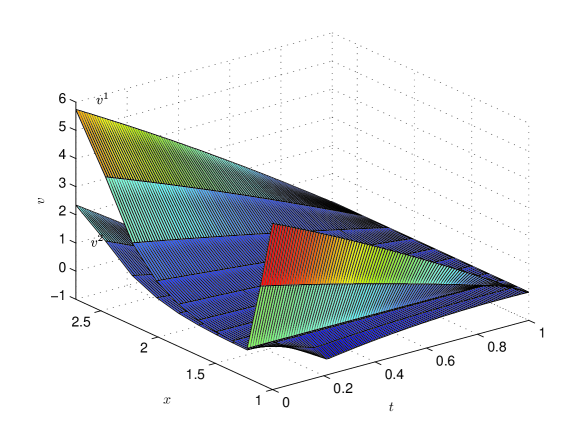
Figure 1: Surfaces of $v^{1}$ and $v^{2}$.

Example 6.2

We now consider the case of 3 modes where $T=1$, $b=x$, $\sigma=\sqrt{2}x$, $g_{12}(t,x)=0$, $g_{13}(t,x)=0$, $g_{21}(t,x)=|x|+t+4$, $g_{23}(t,x)=0$, $g_{31}(t,x)=|x|+t+1$, $g_{32}(t,x)=4t+0.5$, $\psi_{1}(t,x)=x+2t+1$, $\psi_{2}(t,x)=-x+t-2$ and finally $\psi_{3}(t,x)=-x+t-2$.

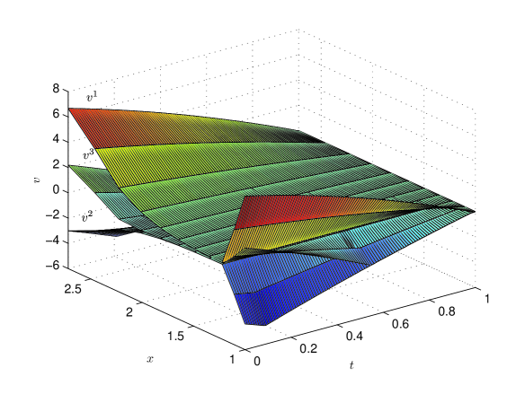
Figure 2: Surfaces of $v^{1}$, $v^{3}$ and $v^{2}$.

7 Appendix

$Proof$ of Lemma 3.1. From (3.3) we have for any $i\in\mathcal{I}$ and $0\leq t\leq T$

(7.1) $$Y_{t}^{i}=\mathop{\mathrm{e}sssup}_{\tau\geq t}E\left[\int_{t}^{\tau}\psi_{i}(s,X_{s})ds+\max\limits_{j\in\mathcal{I}^{-i}}(-g_{ij}(\tau,X_{\tau})+Y_{\tau}^{j})\mathbf{1}_{[\tau<T]}|\mathcal{F}_{t}\right].$$

This also means that the process $(Y_{t}^{i}+\int_{0}^{t}\psi_{i}(s,X_{s})ds)_{0\leq t\leq T}$ is a supermartingale which dominates

$$\left(\int_{0}^{t}\psi_{i}(s,X_{s})ds+\max\limits_{j\in\mathcal{I}^{-i}}(-g_{ij}(t,X_{t})+Y_{t}^{j})\mathbf{1}_{[t<T]}\right)_{0\leq t\leq T}.$$

This implies that the process $(\mathbf{1}_{[u_{\tau_{1}^{\ast}}=i]}(Y_{t}^{i}+\int_{\tau_{1}^{\ast}}^{t}\psi_{i}(s,X_{s})ds))_{t\geq\tau_{1}^{\ast}}$ is a supermartingale which dominates

$$\left(\mathbf{1}_{[u_{\tau_{1}^{\ast}}=i]}\int_{\tau_{1}^{\ast}}^{t}\psi_{i}(s,X_{s})ds+\max\limits_{j\in\mathcal{I}^{-i}}(-g_{ij}(s,X_{t})+Y_{t}^{j})\mathbf{1}_{[t<T]}\right)_{t\geq\tau_{1}^{\ast}}.$$

Since $\mathcal{I}$ is finite, the process $(\sum_{i\in\mathcal{I}}\mathbf{1}_{[u_{\tau_{1}^{\ast}}=i]}(Y_{t}^{i}+\int_{\tau_{1}^{\ast}}^{t}\psi_{i}(s,X_{s})ds))_{t\geq\tau_{1}^{\ast}}$ is also a supermartingale which dominates

$$\left(\sum_{i\in\mathcal{I}}\mathbf{1}_{[u_{\tau_{1}^{\ast}}=i]}\int_{\tau_{1}^{\ast}}^{t}\psi_{i}(s,X_{s})ds+\max\limits_{j\in\mathcal{I}^{-i}}(-g_{ij}(t,X_{t})+Y_{t}^{j})\mathbf{1}_{[t<T]}\right)_{t\geq\tau_{1}^{\ast}}.$$

Thus, the process $Y_{t}^{u_{\tau_{1}^{\ast}}}+\int_{\tau_{1}^{\ast}}^{t}\psi_{u_{\tau_{1}^{\ast}}}(s,X_{s})ds)_{t\geq\tau_{1}^{\ast}}$ is a supermartingale which is greater than

$$\left(\int_{\tau_{1}^{\ast}}^{t}\psi_{u_{\tau_{1}^{\ast}}}(s,X_{s})ds+\max\limits_{j\in\mathcal{I}^{-u_{\tau_{1}^{\ast}}}}(-g_{u_{\tau_{1}^{\ast}}j}(t,X_{t})+Y_{t}^{j})\mathbf{1}_{[t<T]}\right)_{t\geq\tau_{1}^{\ast}}.$$

To complete the proof it remains to show that it is the smallest one which has this property and use the characterization of the Snell envelope see e.g. [4, 17, 19].
Indeed, let $(Z_{t})_{0\leq t\leq T}$ be a supermartingale of class $[D]$ such that, for any $\tau_{1}^{\ast}\leq t\leq T$,

$$Z_{t}\geq\int_{\tau_{1}^{\ast}}^{t}\psi_{u_{\tau_{1}^{\ast}}}(s,X_{s})ds+\max\limits_{j\in\mathcal{I}^{-u_{\tau_{1}^{\ast}}}}(-g_{u_{\tau_{1}^{\ast}}j}(t,X_{t})+Y_{t}^{j})\mathbf{1}_{[t<T]}.$$

It follows that for every $\tau_{1}^{\ast}\leq t\leq T$,

$$\mathbf{1}_{[u_{\tau_{1}^{\ast}}=i]}Z_{t}\geq\mathbf{1}_{[u_{\tau_{1}^{\ast}}=i]}\left(\int_{\tau_{1}^{\ast}}^{t}\psi_{i}(s,X_{s})ds+\max\limits_{j\in\mathcal{I}^{-i}}(-g_{ij}(t,X_{t})+Y_{t}^{j})\mathbf{1}_{[t<T]}\right).$$

But, the process $(\mathbf{1}_{[u_{\tau_{1}^{\ast}}=i]}Z_{t})_{t\geq\tau_{1}^{\ast}}$ is a supermartingale and for every $t\geq\tau_{1}^{\ast}$,

$$\mathbf{1}_{[u_{\tau_{1}^{\ast}}=i]}Y_{t}^{i}=\mathop{\mathrm{e}sssup}_{\tau\geq t}E\left[\mathbf{1}_{[u_{\tau_{1}^{\ast}}=i]}\left(\int_{t}^{\tau}\psi_{i}(s,X_{s})ds+\max\limits_{j\in\mathcal{I}^{-i}}(-g_{ij}(\tau,X_{\tau})+Y_{\tau}^{j})\mathbf{1}_{[\tau<T]}\right)|\mathcal{F}_{t}\right].$$

It follows that, for every $\tau_{1}^{\ast}\leq t\leq T$,

$$\mathbf{1}_{[u_{\tau_{1}^{\ast}}=i]}Z_{t}\geq\mathbf{1}_{[u_{\tau_{1}^{\ast}}=i]}(Y_{t}^{i}+\int_{\tau_{1}^{\ast}}^{t}\psi_{i}(s,X_{s})ds).$$

Summing over $i$, we get, for every $\tau_{1}^{\ast}\leq t\leq T$,

$$Z_{t}\geq Y_{t}^{u_{\tau_{1}^{\ast}}}+\int_{\tau_{1}^{\ast}}^{t}\psi_{u_{\tau_{1}^{\ast}}}(s,X_{s})ds.$$

Hence, the process $(Y_{t}^{u_{\tau_{1}^{\ast}}}+\int_{\tau_{1}^{\ast}}^{t}\psi_{u_{\tau_{1}^{\ast}}}(s,X_{s})ds)_{t\geq\tau_{1}^{\ast}}$ is the Snell envelope of

$$\left(\int_{\tau_{1}^{\ast}}^{t}\psi_{u_{\tau_{1}^{\ast}}}(s,X_{s})ds+\max\limits_{j\in\mathcal{I}^{-u_{\tau_{1}^{\ast}}}}(-g_{u_{\tau_{1}^{\ast}}j}(t,X_{t})+Y_{t}^{j})\mathbf{1}_{[t<T]}\right)_{t\geq\tau_{1}^{\ast}},$$

which completes the proof of the Lemma. $\Box$

References

- [1] B. Bouchard, A stochastic target formulation for optimal switching problems in finite horizon, Stochastics, 81 (2009), pp. 171–197.
- [2] K. A. Brekke and B. Øksendal, Optimal switching in an economic activity under uncertainty. SIAM J. Control Optim, (32) (1994), pp. 1021–1036.
- [3] M. J. Brennan and E. S. Schwartz, Evaluating natural resource investments, J. Business 58 (1985), pp. 135–137.
- [4] J. Cvitanic and I. Karatzas, Backward SDEs with reflection and Dynkin games, Annals of Probability 24 (4) (1996), pp. 2024–2056.
- [5] R. Carmona and M. Ludkovski, Pricing asset scheduling flexibility using optimal switching, Appl. Math. Finance, 15 (2008), pp. 405–447.
- [6] M. Crandall, H. Ishii, H and P.L. Lions, User’s guide to viscosity solutions of second order partial differential equations, Bull. Amer. Math. Soc, 27 (1992), 1–67.
- [7] C. Dellacherie and P. A. Meyer, Probabilités et Potentiel, V-VIII, Hermann, Paris, 1980.
- [8] S. J. Deng and Z. Xia, Pricing and Hedging Electric Supply Contracts: A Case with Tolling Agreements, preprint, Georgia Institute of Technology, Atlanta, 2005.
- [9] A. Dixit, Entry and exit decisions under uncertainty, J. Political Economy, 97 (1989), pp. 620–638.
- [10] A. Dixit and R. S. Pindyck, Investment Under Uncertainty, Princeton University Press, Princeton, NJ, 1994.
- [11] B. Djehiche and S. Hamadène, On a finite horizon starting and stopping problem with risk of abandonment, Int. J. Theor. Appl. Finance, 12 (2009), pp. 523–543.
- [12] B. Djehiche, S. Hamadène, A. Popier, A finite horizon optimal multiple switching problem, SIAM J. Control Optim. 48 (4) (2009) 2751–2770.
- [13] K. Duckworth and M. Zervos, A problem of stochastic impulse control with discretionary stopping, in Proceedings of the 39th IEEE Conference on Decision and Control, IEEE Control Systems Society, Piscataway, NJ, 2000, pp. 222–227.
- [14] K. Duckworth and M. Zervos, A model for investment decisions with switching costs, Ann. Appl. Probab, 11 (2001), pp. 239–260.
- [15] B. El Asri, Optimal Multi-Modes Switching Problem in Infinite Horizon, Stochastics and Dynamics, 10 (2) (2010), pp. 231–261.
- [16] B. El Asri and S. Hamadène, The finite horizon optimal multi-modes switching problem: The viscosity solution approach, Appl. Math. Optim, 60 (2009), pp. 213–235.
- [17] N. El Karoui, Les aspects probabilistes du contrôle stochastique, in Ecole d’été de Probabilités de Saint-Flour, Lecture Notes in Math. 876, Springer-Verlag, New York, 1980.
- [18] N. El Karoui, C. Kapoudjian, E. Pardoux, S. Peng, and M. C. Quenez, Reflected solutions of backward SDEs and related obstacle problems for PDEs, Ann. Probab., 25 (1997), pp. 702–737.
- [19] S. Hamadène, Reflected BSDEs with discontinuous barriers, Stoch. Stoch. Rep., 74 (2002), pp. 571–596.
- [20] S. Hamadène and M. Jeanblanc, On the starting and stopping problem: Application in reversible investments, Math. Oper. Res., 32 (2007), pp. 182–192.
- [21] S. Hamadène and J. Zhang, Switching problem and related system of reflected backward SDEs, Stochastic Processes and their Applications, 120 (2010) 403–426
- [22] Y. Hu and S. Tang, Multi-dimensional BSDE with oblique reflection and optimal switching, Probab. Theory Related Fields (2009) doi:10.1007/s00440-009-0202-1.
- [23] V. Ly Vath and H. Pham, Explicit solution to an optimal switching problem in the two-regime case, SIAM J. Control Optim., 46 (2007), pp. 395–426.
- [24] T. S. Knudsen, B. Meister, and M. Zervos, Valuation of investments in real assets with implications for the stock prices, SIAM J. Control Optim., 36 (1998), pp. 2082–2102.
- [25] A. Porchet, N. Touzi, and X. Warin, Valuation of power plants by utility indifference and numerical computation, Math. Methods Oper. Res., 70 (2009), pp. 47–75.
- [26] D. Revuz and M. Yor, Continuous Martingales and Brownian Motion, Springer-Verlag, Berlin, 1991.
- [27] H. Shirakawa, Evaluation of investment opportunity under entry and exit decisions. Srikaisekikenkysho Kkyroku (987) (1997), pp. 107–124.
- [28] S. Tang and J. Yong, Finite horizon stochastic optimal switching and impulse controls with a viscosity solution approach, Stoch. Stoch. Rep., 45 (1993), pp. 145–176.
- [29] L. Trigeorgis, Real options and interactions with financial flexibility, Financial Management, 22 (1993), pp. 202–224.
- [30] L. Trigeorgis, Real Options: Managerial Flexibility and Strategy in Resource Allocation, MIT Press, Cambridge, MA, 1996.
- [31] M. Zervos, A problem of sequential entry and exit decisions combined with discretionary stopping, SIAM J. Control Optim., 42 (2003), pp. 397–421.