Compressible Distributions
for High-dimensional Statistics

Abstract

We develop a principled way of identifying probability distributions whose independent and identically distributed realizations are compressible, i.e., can be well-approximated as sparse. We focus on Gaussian compressed sensing, an example of underdetermined linear regression, where compressibility is known to ensure the success of estimators exploiting sparse regularization. We prove that many distributions revolving around maximum a posteriori (MAP) interpretation of sparse regularized estimators are in fact incompressible, in the limit of large problem sizes. We especially highlight the Laplace distribution and $\ell^{1}$ regularized estimators such as the Lasso and Basis Pursuit denoising. We rigorously disprove the myth that the success of $\ell^{1}$ minimization for compressed sensing image reconstruction is a simple corollary of a Laplace model of images combined with Bayesian MAP estimation, and show that in fact quite the reverse is true. To establish this result, we identify non-trivial undersampling regions where the simple least squares solution almost surely outperforms an oracle sparse solution, when the data is generated from the Laplace distribution. We also provide simple rules of thumb to characterize classes of compressible and incompressible distributions based on their second and fourth moments. Generalized Gaussian and generalized Pareto distributions serve as running examples.

I Introduction

High-dimensional data is shaping the current modus operandi of statistics. Surprisingly, while the ambient dimension is large in many problems, natural constraints and parameterizations often cause data to cluster along low-dimensional structures. Identifying and exploiting such structures using probabilistic models is therefore quite important for statistical analysis, inference, and decision making.

In this paper, we discuss compressible distributions, whose independent and identically distributed (iid) realizations can be well-approximated as sparse. Whether or not a distribution is compressible is important in the context of many applications, among which we highlight two here: statistics of natural images, and statistical regression for linear inverse problems such as those arising in the context of compressed sensing.

Statistics of natural images

Acquisition, compression, denoising, and analysis of natural images (similarly, medical, seismic, and hyperspectral images) draw high scientific and commercial interest. Research to date in natural image modeling has had two distinct approaches, with one focusing on deterministic explanations and the other pursuing probabilistic models. Deterministic approaches (see e.g. [10, 12]) operate under the assumption that the transform domain representations (e.g., wavelets, Fourier, curvelets, etc.) of images are “compressible”. Therefore, these approaches threshold the transform domain coefficients for sparse approximation, which can be used for compression or denoising.

Existing probabilistic approaches also exploit coefficient decay in transform domain representations, and learn probabilistic models by approximating the coefficient histograms or moment matching. For natural images, the canonical approach (see e.g. [27]) is to fit probability density functions (PDF’s), such as generalized Gaussian distributions and the Gaussian scale mixtures, to the histograms of wavelet coefficients while trying to simultaneously capture the dependencies observed in their marginal and joint distributions.

Statistical regression

Underdetermined linear regression is a fundamental problem in statistics, applied mathematics, and theoretical computer science with broad applications—from subset selection to compressive sensing [17, 7] and inverse problems (e.g., deblurring), and from data streaming to error corrective coding. In each case, we seek an unknown vector $\mathbf{x}\in\mathbb{R}^{N}$, given its dimensionality reducing, linear projection $\mathbf{y}\in\mathbb{R}^{m}$ ($m<N$) obtained via a known encoding matrix $\mathbf{\Phi}\in\mathbb{R}^{m\times N}$, as

$$\mathbf{y}=\mathbf{\Phi}\mathbf{x}+\mathbf{n},$$ (1)

where $\mathbf{n}\in\mathbb{R}^{m}$ accounts for the perturbations in the linear system, such as physical noise. The core challenge in decoding $\mathbf{x}$ from $\mathbf{y}$ stems from the simple fact that dimensionality reduction loses information in general: for any vector $v\in\text{kernel}(\mathbf{\Phi})$, it is impossible to distinguish $\mathbf{x}$ from $\mathbf{x}+v$ based on $\mathbf{y}$ alone.

Prior information on $\mathbf{x}$ is therefore necessary to estimate the true $\mathbf{x}$ among the infinitely many possible solutions. It is now well-known that geometric sparsity models (associated to approximation of $\mathbf{x}$ from a finite union of low-dimensional subspaces in $\mathbb{R}^{N}$ [4]) play an important role in obtaining “good” solutions. A widely exploited decoder is the $\ell^{1}$ decoder $\Delta_{1}(\mathbf{y}):=\arg\min_{\tilde{\mathbf{x}}:\mathbf{y}=\mathbf{\Phi}\tilde{\mathbf{x}}}\|\tilde{\mathbf{x}}\|_{1}$ whose performance can be explained via the geometry of projections of the $\ell^{1}$ ball in high dimensions [16]. A more probabilistic perspective considers $\mathbf{x}$ as drawn from a distribution. As we will see, compressible iid distributions [2, 9] countervail the ill-posed nature of compressed sensing problems by generating vectors that, in high dimensions, are well approximated by the geometric sparsity model.

I-A Sparsity, compressibility and compressible distributions

A celebrated result from compressed sensing [17, 6] is that under certain conditions, a $k$-sparse vector $\mathbf{x}$ (with only $k$ non-zero entries where $k$ is usually much smaller than $N$) can be exactly recovered from its noiseless projection $\mathbf{y}$ using the $\ell^{1}$ decoder, as long as $m\gtrsim k\log N/k$. Possibly the most striking result of this type is the Donoho-Tanner weak phase transition that, for Gaussian sensing matrices, completely characterizes the typical success or failure of the $\ell^{1}$ decoder in the large scale limit [16].

Even when the vector $\mathbf{x}$ is not sparse, under certain “compressibility” conditions typically expressed in terms of (weak) $\ell^{p}$ balls, the $\ell^{1}$-decoder provides estimates with controlled accuracy [13, 8, 14, 18]. Intuitively one should only expect a sparsity-seeking estimator to perform well if the vector being reconstructed is at least approximately sparse. Informally, compressible vectors can be defined as follows:

Definition 1 (Compressible vectors).

Define the relative best $k$-term approximation error $\bar{\sigma}_{k}(\mathbf{x})_{q}$ of a vector $\mathbf{x}$ as

$$\bar{\sigma}_{k}(\mathbf{x})_{q}=\frac{{\sigma}_{k}(\mathbf{x})_{q}}{\|\mathbf{x}\|_{q}},$$ (2)

where $\sigma_{k}(\mathbf{x})_{q}:=\inf_{\|\mathbf{y}\|_{0}\leq k}\|\mathbf{x}-\mathbf{y}\|_{q}$ is the best $k$-term approximation error of $\mathbf{x}$, and $\|\mathbf{x}\|_{q}$ is the $\ell^{q}$-norm of $\mathbf{x}$, $q\in(0,\infty)$. By convention $\|{\mathbf{x}}\|_{0}$ counts the non-zero coefficients of ${\mathbf{x}}$. A vector $\mathbf{x}\in\mathbb{R}^{N}$ is $q$-compressible if $\bar{\sigma}_{k}(\mathbf{x})_{q}\ll 1$ for some $k\ll N$.

This definition of compressibility differs slightly from those that are closely linked to weak $\ell^{p}$ balls in that, above, we consider relative error. This is discussed further in Section III.

When moving from the deterministic setting to the stochastic setting it is natural to ask when reconstruction guarantees equivalent to the deterministic ones exist. The case of typically sparse vectors is most easily dealt with and can be characterized by a distribution with a probability mass of $(1-k/N)$ at zero, e.g., a Bernoulli-Gaussian distribution. Here the results of Donoho and Tanner still apply as a random vector drawn from such a distribution is typically sparse, with approximately $k$ nonzero entries, while the $\ell^{1}$ decoder is blind to the specific non-zero values of $\mathbf{x}$.

The case of compressible vectors is less straightforward: when is a vector generated from iid draws of a given distribution typically compressible? This is the question investigated in this paper. To exclude the sparse case, we restrict ourselves to distributions with a well defined density $p(x)$.

Broadly speaking, we can define compressible distributions as follows.

Definition 2 (Compressible distributions).

Let $X_{n}(n\in\mathbb{N})$ be iid samples from a probability distribution with probability density function (PDF) $p(x)$, and $\mathbf{x}_{N}=(X_{1},\ldots,X_{N})\in\mathbb{R}^{N}$. The PDF $p(x)$ is said to be $q$-compressible with parameters $(\epsilon,\kappa)$ when

$$\limsup_{N\to\infty}\bar{\sigma}_{k_{N}}(\mathbf{x}_{N})_{q}\stackrel{{\scriptstyle a.s.}}{{\leq}}\epsilon,(\text{a.s.: almost surely});$$ (3)

for any sequence $k_{N}$ such that $\liminf_{N\to\infty}\frac{k_{N}}{N}\geq\kappa$.

The case of interest is when $\epsilon\ll 1$ and $\kappa\ll 1$: iid realizations of a $q$-compressible distribution with parameters $(\epsilon,\kappa)$ live in $\epsilon$-proximity to the union of $\kappa N$-dimensional hyperplanes, where the closeness is measured in the $\ell^{q}$-norm. These hyperplanes are aligned with the coordinate axes in $N$-dimensions.

One can similarly define an incompressible distribution as:

Definition 3 (Incompressible distributions).

Let $X_{n}$ and $\mathbf{x}_{N}$ be defined as above. The PDF $p(x)$ is said to be $q$-incompressible with parameters $(\epsilon,\kappa)$ when

$$\liminf_{N\to\infty}\bar{\sigma}_{k_{N}}(\mathbf{x}_{N})_{q}\stackrel{{\scriptstyle a.s.}}{{\geq}}\epsilon,$$ (4)

for any sequence $k_{N}$ such that $\limsup_{N\to\infty}\frac{k_{N}}{N}\leq\kappa$.

This states that the iid realizations of an incompressible distribution live away from the $\epsilon$-proximity of the union of $\kappa N$-dimensional hyperplanes, where $\epsilon\approx 1$.

More formal characterizations of the “compressibility” or the “incompressibility” of a distribution with PDF $p(x)$ are investigated in this paper. With a special emphasis on the context of compressed sensing with a Gaussian encoder $\mathbf{\Phi}$, we discuss and characterize the compatibility of such distributions with extreme levels of undersampling. As a result, our work features both positive and negative conclusions on achievable approximation performance of probabilistic modeling in compressed sensing.

I-B Structure of the paper

The main results are stated in Section II together with a discussion of their conceptual implications. The section is concluded by Table I, which provides an overview at a glance of the results. The following sections discuss in more details our contributions, while the bulk of the technical contributions is gathered in an appendix, to allow the main body of the paper to concentrate on the conceptual implications of the results. As running examples, we focus on the Laplace distribution for incompressibility and the generalized Pareto distribution for compressibility, with a Gaussian encoder $\mathbf{\Phi}$.

II Main results

In this paper, we aim at bringing together the deterministic and probabilistic models of compressibility in a simple and general manner under the umbrella of compressible distributions. To achieve our goal, we dovetail the concept of order statistics from probability theory with the deterministic models of compressibility from approximation theory.

Our five “take home” messages for compressed sensing are as follows:

1. $\ell^{1}$ minimization does not assume that the underlying coefficients have a Laplace distribution. In fact, the relatively flat nature of vectors drawn iid from a Laplace distribution makes them, in some sense, the worst for compressed sensing problems.

2. It is simply not true that the success of $\ell^{1}$ minimization for compressed sensing reconstruction is a simple corollary of a Laplace model of data coefficients combined with Bayesian MAP estimation, in fact quite the reverse.

3. Even with the strongest possible recovery guarantees [13, 14], compressed sensing reconstruction of Laplace distributed vectors with the $\ell^{1}$ decoder offers no guarantees beyond the trivial estimator, $\widehat{\mathbf{x}}=0$.

4. More generally, for high-dimensional vectors $\mathbf{x}$ drawn iid from any density with bounded fourth moment $\mathbb{E}X^{4}<\infty$, even with the help of a sparse oracle, there is a critical level of undersampling below which the sparse oracle estimator is worse (in relative $\ell^{2}$ error) than the simple least-squares estimator.

5. In contrast, when a high-dimensional vector $\mathbf{x}$ is drawn from a density with infinite second moment $\mathbb{E}X^{2}=\infty$, then the $\ell^{1}$ decoder can reconstruct $\mathbf{x}$ with arbitrarily small relative $\ell^{2}$ error.

II-A Relative sparse approximation error

By using Wald’s lemma on order statistics, we characterize the relative sparse approximation errors of iid PDF realizations, whereby providing solid mathematical ground to the earlier work of Cevher [9] on compressible distributions. While Cevher exploits the decay of the expected order statistics, his approach is inconclusive in characterizing the “incompressibility” of distributions. We close this gap by introducing a function $G_{q}[p](\kappa)$ so that iid vectors as in Definition 2 satisfy $\lim_{N\to\infty}\bar{\sigma}_{k_{N}}(\mathbf{x}_{N})_{q}^{q}\stackrel{{\scriptstyle a.s.}}{{=}}G_{q}[p](\kappa)$ when $\lim_{N\to\infty}k_{N}/N=\kappa\in(0,1)$.

Proposition 1.

Suppose $\mathbf{x}_{N}\in\mathbb{R}^{N}$ is iid with respect to $p(x)$ as in Definition 2. Denote $\bar{p}(x):=0$ for $x<0$, and $\bar{p}(x):=p(x)+p(-x)$ for $x\geq 0$ as the PDF of $|X_{n}|$, and $\bar{F}(t):=\mathbb{P}(|X|\leq t)$ as its cumulative density function (CDF). Assume that $\bar{F}$ is continuous and strictly increasing on some interval $[a\ b]$, with $\bar{F}(a)=0$ and $\bar{F}(b)=1$, where $0\leq a<b\leq\infty$. For any $0<\kappa\leq 1$, define the following function:

$$G_{q}[p](\kappa):=\frac{\int_{0}^{\bar{F}^{-1}(1-\kappa)}x^{q}\bar{p}(x)dx}{\int_{0}^{\infty}x^{q}\bar{p}(x)dx}.$$ (5)

1. Bounded moments: assume $\mathbb{E}|X|^{q}<\infty$ for some $q\in(0,\infty)$. Then, $G_{q}[p](\kappa)$ is also well defined for $\kappa=0$, and for any sequence $k_{N}$ such that $\lim_{N\to\infty}\frac{k_{N}}{N}=\kappa\in[0,1]$, the following holds almost surely

   $$\lim_{N\to\infty}\bar{\sigma}_{k_{N}}(\mathbf{x}_{N})_{q}^{q}\stackrel{{\scriptstyle a.s.}}{{=}}G_{q}[p](\kappa).$$ (6)

2. Unbounded moments: assume $\mathbb{E}|X|^{q}=\infty$ for some $q\in(0,\infty)$. Then, for $0<\kappa\leq 1$ and any sequence $k_{N}$ such that $\lim_{N\to\infty}\frac{k_{N}}{N}=\kappa$, the following holds almost surely

   $$\lim_{N\to\infty}\bar{\sigma}_{k_{N}}(\mathbf{x}_{N})_{q}^{q}\stackrel{{\scriptstyle a.s.}}{{=}}G_{q}[p](\kappa)=0.$$ (7)

Proposition 1 provides a principled way of obtaining the compressibility parameters $(\epsilon,\kappa)$ of distributions in the high dimensional scaling of the vectors. An immediate application is the incompressibility of the Laplace distribution.

Example 1.

As a stylized example, consider the Laplace distribution (also known as the double exponential) with scale parameter 1, whose PDF is given by

$$p_{1}(x):=\frac{1}{2}\exp(-|x|).$$ (8)

We compute in Appendix -I:

$$G_{1}[p_{1}](\kappa) =1-\kappa\cdot\Big{(}1+\ln 1/\kappa\Big{)},$$ (9)

$$G_{2}[p_{1}](\kappa) =1-\kappa\cdot\Big{(}1+\ln 1/\kappa+\frac{1}{2}(\ln 1/\kappa)^{2}\Big{)}.$$ (10)

Therefore, it is straightforward to see that the Laplace distribution is not $q$-compressible for $q\in\{1,2\}$: it is not possible to simultaneously have both $\kappa$ and $\epsilon=G_{q}[p_{1}](\kappa)$ small.

II-B Sparse modeling vs. sparsity promotion

We show that the maximum a posteriori (MAP) interpretation of standard deterministic sparse recovery algorithms is, in some sense, inconsistent. To explain why, we consider the following decoding approaches to estimate a vector $\mathbf{x}$ from its encoding $\mathbf{y}=\mathbf{\Phi}\mathbf{x}$:

$$\Delta_{1}(\mathbf{y}) =\operatorname*{argmin}_{\tilde{\mathbf{x}}:\mathbf{y}=\mathbf{\Phi}\tilde{\mathbf{x}}}\|\tilde{\mathbf{x}}\|_{1},$$ (11)

$$\Delta_{\textrm{LS}}(\mathbf{y}) =\operatorname*{argmin}_{\tilde{\mathbf{x}}:\mathbf{y}=\mathbf{\Phi}\tilde{\mathbf{x}}}\|\tilde{\mathbf{x}}\|_{2}=\mathbf{\Phi}^{+}\mathbf{y},$$ (12)

$$\Delta_{\textrm{oracle}}(\mathbf{y},\Lambda) =\operatorname*{argmin}_{\tilde{\mathbf{x}}:\textrm{support}(\tilde{\mathbf{x}})=\Lambda}\|\mathbf{y}-\mathbf{\Phi}\tilde{\mathbf{x}}\|_{2}=\mathbf{\Phi}_{\Lambda}^{+}\mathbf{y},$$ (13)

$$\Delta_{\textrm{trivial}}(\mathbf{y}) =0.$$ (14)

Here, $\mathbf{\Phi}_{\Lambda}$ denotes the sub-matrix of $\mathbf{\Phi}$ restricted to the columns indexed by the set $\Lambda$. The decoder $\Delta_{1}$ regularizes the solution space via the $\ell^{1}$-norm. It is the de facto standard Basis Pursuit formulation [11] for sparse recovery, and is tightly related to the Basis Pursuit denoising (BPDN) and the least absolute shrinkage and selection operator (LASSO) [31]:

$$\Delta_{\text{BPDN}}(\mathbf{y}) =\operatorname*{argmin}_{\tilde{\mathbf{x}}}\left\{\frac{1}{2}\|\mathbf{y}-\mathbf{\Phi}\tilde{\mathbf{x}}\|_{2}^{2}+\lambda\|\tilde{\mathbf{x}}\|_{1}\right\}$$

where $\lambda$ is a constant. Both $\Delta_{1}$ and the BPDN formulations can be solved in polynomial time through convex optimization techniques. The decoder $\Delta_{\textrm{LS}}$ is the traditional minimum least-squares solution, which is related to the Tikhonov regularization or ridge regression. It uses the Moore-Penrose pseudo-inverse $\mathbf{\Phi}^{+}=\mathbf{\Phi}^{T}(\mathbf{\Phi}\mathbf{\Phi}^{T})^{-1}$. The oracle sparse decoder $\Delta_{\textrm{oracle}}$ can be seen as an idealization of sparse decoders, which combine subset selection (the choice of $\Lambda$) with a form of linear regression. It is an “informed” decoder that has the side information of the index set $\Lambda$ associated with the largest components in $\mathbf{x}$. The trivial decoder $\Delta_{\textrm{trivial}}$ plays the devil’s advocate for the performance guarantees of the other decoders.

II-B1 Almost sure performance of decoders

When the encoder $\mathbf{\Phi}$ provides near isometry to the set of sparse vectors [6], the decoder $\Delta_{1}$ features an instance optimality property [13, 14]:

$$\|\Delta_{1}(\mathbf{\Phi}\mathbf{x})-\mathbf{x}\|_{1}\leq C_{k}(\mathbf{\Phi})\cdot\sigma_{k}(\mathbf{x})_{1},\forall\mathbf{x};$$ (15)

where $C_{k}(\mathbf{\Phi})$ is a constant which depends on $\mathbf{\Phi}$. A similar result holds with the $\|\cdot\|_{2}$ norm on the left hand side. Unfortunately, it is impossible to have the same uniform guarantee for all $\mathbf{x}$ with $\sigma_{k}(\mathbf{x})_{2}$ on the right hand side [13], but for any given $\mathbf{x}$, it becomes possible in probability [13, 15]. For a Gaussian encoder, $\Delta_{1}$ recovers exact sparse vectors perfectly from as few as $m\approx 2ek\log N/k$ with high probability [16].

Definition 4 (Gaussian encoder).

Let $\phi_{i,j}$, $i,j\in\mathbb{N}$ be iid Gaussian variables $\mathcal{N}(0,1)$. The $m\times N$ Gaussian encoder is the random matrix $\mathbf{\Phi}_{N}:=\left[\phi_{ij}/\sqrt{m}\right]_{1\leq i\leq m,1\leq j\leq N}$.

In the sequel, we only consider the Gaussian encoder, leading to Gaussian compressed sensing (G-CS) problems. In Section IV, we theoretically characterize the almost sure performance of the estimators $\Delta_{\textrm{LS}}$, $\Delta_{\textrm{oracle}}$ for arbitrary high-dimensional vectors $\mathbf{x}$. We concentrate our analysis to the noiseless setting ($\mathbf{n}=0$). The least squares decoder $\Delta_{\textrm{LS}}$ has expected performance $\mathbb{E}_{\mathbf{\Phi}}\|\Delta_{\textrm{LS}}(\mathbf{\Phi}\mathbf{x})-\mathbf{x}\|_{2}^{2}/\|\mathbf{x}\|_{2}^{2}=1-\delta$, independent of the vector $\mathbf{x}$, where

$$\delta:=m/N$$ (16)

is the undersampling ratio associated to the matrix $\mathbf{\Phi}$ (this terminology comes from compressive sensing, where $\mathbf{\Phi}$ is a sampling matrix). In theorem 3 the expected performance of the oracle sparse decoder $\Delta_{\textrm{oracle}}$ is shown to satisfy

$$\frac{\mathbb{E}_{\mathbf{\Phi}}\|\Delta_{\textrm{oracle}}(\mathbf{\Phi}\mathbf{x},\Lambda)-\mathbf{x}\|_{2}^{2}}{\|\mathbf{x}\|_{2}^{2}}=\frac{1}{1-\frac{k}{m-1}}\times\frac{\sigma_{k}(\mathbf{x})^{2}}{\|\mathbf{x}\|_{2}^{2}}.$$

This error is the balance between two factors. The first factor grows with $k$ (the size of the set $\Lambda$ of largest entries of $\mathbf{x}$ used in the decoder) and reflects the (ill-)conditioning of the Gaussian submatrix $\mathbf{\Phi}_{\Lambda}$. The second factor is the best $k$-term relative approximation error, which shrinks as $k$ increases. This highlights the inherent trade-off present in any sparse estimator, namely the level of sparsity $k$ versus the conditioning of the sub-matrices of $\mathbf{\Phi}$.

II-B2 A few surprises regarding sparse recovery guarantees

We highlight two counter-intuitive results below:

A crucial weakness in appealing to instance optimality

Although instance optimality (15) is usually considered as a strong property, it involves an implicit trade off: when $k$ is small, the $k$-term error $\sigma_{k}(\mathbf{x})$ is large, while for larger $k$, the constant $C_{k}(\mathbf{\Phi})$ is large. For instance, we have $C_{k}(\mathbf{\Phi})=\infty$, when $k\geq m$.

In Section III we provide new key insights for instance optimality of algorithms. Informally, we show that when $\mathbf{x}_{N}\in\mathbb{R}^{N}$ is iid with respect to $p(x)$ as in Definition 2, and when $p(x)$ satisfies the hypotheses of Proposition 1, if

$$G_{1}[p](\kappa_{0})\geq 1/2,$$ (17)

where $\kappa_{0}\approx 0.18$ is an absolute constant, then the best possible upper bound in the instance optimality (15) for a Gaussian encoder satisfies (in the limit of large $N$)

$$C_{k}(\mathbf{\Phi})\cdot\sigma_{k}(\mathbf{x})_{1}\geq\|\mathbf{x}\|_{1}=\|\Delta_{\textrm{trivial}}(\mathbf{x})-\mathbf{x}\|_{1}.$$

In other words, for distributions with PDF $p(x)$ satisfying (17), in high dimension $N$, instance optimality results for the decoder $\Delta_{1}$ with a Gaussian encoder can at best guarantee the performance (in the $\ell^{1}$ norm) of the trivial decoder $\Delta_{\textrm{trivial}}$!

Condition (17) holds true for many general PDF’s; it is easily verifiable for the Laplace distribution based on Example 1, and explains the observed failure of the $\ell^{1}$ decoder on Laplace data [29]. This is discussed further in Section III.

Fundamental limits of sparsity promoting decoders

The expected $\ell^{2}$ relative error of the least-squares estimator $\Delta_{\textrm{LS}}$ degrades linearly as $1-\delta$ with the undersampling factor $\delta:=m/N$, and therefore does not provide good reconstruction at low sampling rates $\delta\ll 1$. It is therefore quite surprising that we can determine a large class of distributions for which the oracle sparse decoder $\Delta_{\textrm{oracle}}$ is outperformed by the simple least-squares decoder $\Delta_{\textrm{LS}}$.

Theorem 1.

Suppose that $\mathbf{x}_{N}\in\mathbb{R}^{N}$ is iid with respect to $p(x)$ as in Definition 2, and that $p(x)$ satisfies the hypotheses of Proposition 1 and has a finite fourth-moment

$$\mathbb{E}X^{4}<\infty.$$

There exists a minimum undersampling ratio $\delta_{0}$ with the following property: for any $\rho\in(0,1)$, if $\mathbf{\Phi}_{N}$ is a sequence of $m_{N}\times N$ Gaussian encoders with $\lim_{N\to\infty}m_{N}/N=\delta<\delta_{0}$, and $\lim_{N\to\infty}k_{N}/m_{N}=\rho$, then we have almost surely

$$\lim_{N\to\infty} \frac{\|\Delta_{\textrm{oracle}}(\mathbf{\Phi}_{N}\mathbf{x}_{N},\Lambda_{N})-\mathbf{x}_{N}\|_{2}^{2}}{\|\mathbf{x}_{N}\|_{2}^{2}}$$

$$\stackrel{{\scriptstyle a.s.}}{{=}}\frac{G_{2}[p](\rho\delta)}{1-\rho}$$

$$>1-\delta\stackrel{{\scriptstyle a.s.}}{{=}}\lim_{N\to\infty}\frac{\|\Delta_{\textrm{LS}}(\mathbf{\Phi}_{N}\mathbf{x}_{N})-\mathbf{x}_{N}\|_{2}^{2}}{\|\mathbf{x}_{N}\|_{2}^{2}}.$$

Thus if the data PDF $p(x)$ has a finite fourth moment and a continuous CDF, there exists a level of undersampling below which a simple least-squares reconstruction (typically a dense vector estimate) provides an estimate, which is closer to the true vector $\mathbf{x}$ (in the $\ell^{2}$ sense) than oracle sparse estimation!

Section V describes how to determine this undersampling boundary, e.g., for the generalized Gaussian distribution. For the Laplace distribution, $\delta_{0}\approx 0.15$. In other words, when randomly sampling a high-dimensional Laplace vector, it is better to use least-squares reconstruction than minimum $\ell^{1}$ norm reconstruction (or any other type of sparse estimator), unless the number of measures $m$ is at least $15\%$ of the original vector dimension $N$. To see how well Theorem 1 is grounded in practice, we provide the following example:

Example 2.

Figure 1 examines in more detail the performance of the estimators for Laplace distributed data at various undersampling values. The horizontal lines indicate various signal-to-distortion-ratios (SDR) of $3$dB, $10$dB and $20$dB. Thus for the oracle estimator to achieve $10$dB, the undersampling rate must be greater than 0.7, while to achieve a performance level of $20$dB, something that might reasonably be expected in many compressed sensing applications, we can hardly afford any subsampling at all since this requires $\delta>0.9$.

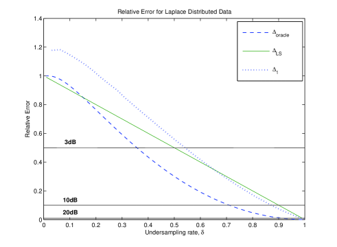
Figure 1: The expected relative error as a function of the undersampling rates $\delta$ for data iid from a Laplace distribution using: (a) a linear least squares estimator (solid) and (b) the best oracle sparse estimator (dashed). Also plotted is the empirically observed average relative error over 5000 instances for the $\Delta_{1}$ estimator (dotted). The horizontal lines indicate SDR values of $3$dB, $10$dB and $20$dB, as marked.

This may come as a shock since, in Bayesian terminology, $\ell^{1}$-norm minimization is often conventionally interpreted as the MAP estimator under the Laplace prior, while least squares is the MAP under the Gaussian prior. Such MAP interpretations of compressed sensing decoders are further discussed below and contrasted to more geometric interpretations.

II-C Pitfalls of MAP “interpretations” of decoders

Bayesian compressed sensing methods employ probability measures as “priors” in the space of the unknown vector $\mathbf{x}$, and arbitrate the solution space by using the chosen measure. The decoder $\Delta_{1}$ has a distinct probabilistic interpretation in the statistics literature. If we presume an iid probabilistic model for $\mathbf{x}$ as $p(X_{n})\propto\exp\left(-c|X_{n}|\right)$ ($n=1,\ldots,N$), then $\Delta_{\text{BPDN}}$ can be viewed as the MAP estimator

$$\Delta_{\textrm{MAP}}(\mathbf{y}):=\arg\max_{\mathbf{x}}p(\mathbf{x}|\mathbf{y})=\arg\min_{\mathbf{x}}\{-\log p(\mathbf{x}|\mathbf{y})\},$$

when the noise $\mathbf{n}$ is iid Gaussian, which becomes the $\Delta_{1}$ decoder in the zero noise limit. However, as illustrated by Example 2, the decoder $\Delta_{\textrm{MAP}}$ performs quite poorly for iid Laplace vectors. The possible inconsistency of MAP estimators is a known phenomenon [26]. Yet, the fact that $\Delta_{\textrm{MAP}}$ is outperformed by $\Delta_{\textrm{LS}}$—which is the MAP under the Gaussian prior—when $\mathbf{x}$ is drawn iid according to the Laplacian distribution should remain somewhat counterintuitive to many readers.

It is now not uncommon to stumble upon new proposals in the literature for the modification of $\Delta_{1}$ or BPDN with diverse thresholding or re-weighting rules based on different hierarchical probabilistic models—many of which correspond to a special Bayesian “sparsity prior” $p(\mathbf{x})\propto\exp(-\phi(\mathbf{x}))$ [32], associated to the minimization of new cost functions

$$\Delta_{\phi}(\mathbf{y}):=\arg\min_{\mathbf{x}}\frac{1}{2}\|\mathbf{y}-\mathbf{\Phi}\mathbf{x}\|_{2}^{2}+\phi(\mathbf{x}).$$

It has been shown in the context of additive white Gaussian noise denoising that the MAP interpretation of such penalized least-squares regression can be misleading [20]. Just as illustrated above with $\phi(\mathbf{x})=\lambda\|\mathbf{x}\|_{1}$, while the geometric interpretations of the cost functions associated to such “priors” are useful for sparse recovery, the “priors” $\exp(-\phi(\mathbf{x}))$ themselves do not necessarily constitute a relevant “generative model” for the vectors. Hence, such proposals are losing a key strength of the Bayesian approach: the ability to evaluate the “goodness” or “confidence” of the estimates due to the probabilistic model itself or its conjugate prior mechanics.

In fact, the empirical success of $\Delta_{1}$ (or $\Delta_{\text{BPDN}}$) results from a combination of two properties:

1. the sparsity-inducing nature of the cost function, due to the non-differentiability at zero of the $\ell^{1}$ cost function;

2. the compressible nature of the vector $\mathbf{x}$ to be estimated.

Geometrically speaking, the objective $\|{\mathbf{x}}\|_{1}$ is related to the $\ell^{1}$-ball, which intersects with the constraints (e.g., a randomly oriented hyperplane, as defined by $\mathbf{y}=\mathbf{\Phi}\mathbf{x}$) along or near the $k$-dimensional hyperplanes ($k\ll N$) that are aligned with the canonical coordinate axes in $\mathbb{R}^{N}$. The geometric interplay of the objective and the constraints in high-dimensions inherently promotes sparsity. An important practical consequence is the ability to design efficient optimization algorithms for large-scale problems, using thresholding operations. Therefore, the decoding process of $\Delta_{1}$ automatically sifts smaller subsets that best explain the observations, unlike the traditional least-squares $\Delta_{\textrm{LS}}$.

When $\mathbf{x}_{N}$ has iid coordinates as in Definition 2, compressibility is not so much related to the behavior (differentiable or not) of $p(x)$ around zero but rather to the thickness of its tails, e.g., through the necessary property $\mathbb{E}X^{4}=\infty$ (cf Theorem 1). We further show that distributions with infinite variance ($\mathbb{E}X^{2}=\infty$) almost surely generate vectors which are sufficiently compressible to guarantee that the decoder $\Delta_{1}$ with a Gaussian encoder $\mathbf{\Phi}$ of arbitrary (fixed) small sampling ratio $\delta=m/N$ has ideal performance in dimensions $N$ growing to infinity:

Theorem 2 (Asymptotic performance of the $\ell^{1}$ decoder under infinite second moment).

Suppose that $\mathbf{x}_{N}\in\mathbb{R}^{N}$ is iid with respect to $p(x)$ as in Definition 2, and that $p(x)$ satisfies the hypotheses of Proposition 1 and has infinite second moment $\mathbb{E}X^{2}=\infty$. Consider a sequence of integers $m_{N}$ such that $\lim_{N\to\infty}m_{N}/N=\delta$ where $0<\delta<1$ is arbitrary, and let $\mathbf{\Phi}_{N}$ be a sequence of $m_{N}\times N$ Gaussian encoders. Then

$$\lim_{N\to\infty}\frac{\|\Delta_{1}(\mathbf{\Phi}_{N}\mathbf{x}_{N})-\mathbf{x}_{N}\|_{2}}{\|\mathbf{x}_{N}\|_{2}}\stackrel{{\scriptstyle a.s.}}{{=}}0.$$ (18)

As shown in Section VI there exist PDFs $p(x)$, which combine heavy tails with a non-smooth behavior at zero, such that the associated MAP estimator is sparsity promoting. It is likely that the MAP with such priors can be shown to perform ideally well in the asymptotic regime.

TABLE I: Summary of the main results

Moment property	$\mathbb{E}X^{2}=\infty$	$\mathbb{E}X^{2}<\infty$ and $\mathbb{E}X^{4}=\infty$	$\mathbb{E}X^{4}<\infty$
	Theorem 2	N/A	Theorem 1
General result	$\Delta_{1}$ performs ideally	depends on finer	$\Delta_{\textrm{LS}}$ outperforms $\Delta_{\textrm{oracle}}$
	for any $\delta$	properties of $p(x)$	for small $\delta<\delta_{0}$
Compressible	YES	YES or NO	NO
		Proposition 2 (Section V-A):	Section V-B:
		$p_{0}(x):=2|x|/(x^{2}+1)^{3}$	$p_{\tau}(x)\propto\exp(-|x|^{\tau})$
			$0<\tau<\infty$
		$\Delta_{\textrm{oracle}}$ performs just as $\Delta_{\textrm{LS}}$	Generalized Gaussian
Examples
	Example 4 (Section VI):
	$p_{\tau,s}(x)\propto(1+|x|^{\tau})^{-s/\tau}$
	Generalized Pareto ($\tau=1$) / Student’s $t$ ($\tau=2$)
2-4	Case $1<s\leq 3$	Case $3<s<5$	Case $s>5$
		$\Delta_{\textrm{oracle}}$ outperforms $\Delta_{\textrm{LS}}$
		for small $\delta<\delta_{0}$

II-D Are natural images compressible or incompressible ?

Theorems 1 and 2 provide easy to check conditions for (in)compressibility of a PDF $p(x)$ based on its second of fourth moments. These rules of thumb are summarized in Table I, providing an overview at a glance of the main results obtained in this paper.

We conclude this extended overview of the results with stylized application of these rules of thumb to wavelet and discrete cosine transform (DCT) coefficients of the natural images from the Berkeley database [24]. Our results below provide an approximation theoretic perspective to the probabilistic modeling approaches in natural scene statistics community [28, 30, 27].

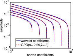
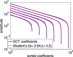
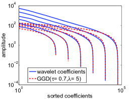
(a) Wavelet/GPD	(b) DCT/Student’s $t$ distribution	(c) Wavelet/GGD

Figure 2: Solid lines illustrate the Wavelet or DCT transform domain average order statistics of image patches from the Berkeley database [24]. Dashed lines show the theoretical expected order statistics of the GPD, Student’s $t$, and the GGD distributions with the indicated parameter values. The resolution of image patch sizes varies from left to right as $\{(8\times 8),(16\times 16),\ldots,(256\times 256)\}$, respectively.

Figure 2 illustrates, in log-log scale, the average of the magnitude ordered wavelet coefficients (Figures 2-(a)-(c)), and of the DCT coefficients (Figure 2-(b)). They are obtained by randomly sampling $100$ image patches of varying sizes $N=2^{j}\times 2^{j}$ ($j=3,\ldots,8$), and taking their transforms (scaling filter for wavelets: Daubechies4). For comparison, we also plot the expected order statistics (dashed lines), as described in [9], of the following distributions (cf Sections V-B and VI)

• GPD: the scaled generalized Pareto distribution with density $\frac{1}{\lambda}p_{\tau,s}(x/\lambda)$, $\tau=1$, with parameters $s=2.69$ and $\lambda=8$ (Figure 2-(a));

• Student’s $t$: the scaled Student’s $t$ distribution with density $\frac{1}{\lambda}p_{\tau,s}(x/\lambda)$, $\tau=2$, with parameters $s=2.64$ and $\lambda=4.5$ (Figure 2-(b));

• GGD: the scaled generalized Gaussian distribution with density $\frac{1}{\lambda}p_{\tau}(x/\lambda)$, with $\tau=0.7$ and $\lambda=5$ (Figure 2-(c)).

The GGD parameters were obtained by approximating the histogram of the wavelet coefficients at $N=8\times 8$, as it is the common practice in the signal processing community [10]. The GPD and Student’s $t$ parameters were tuned manually.

One should note that image transform coefficients are certainly not iid [29], for instance: nearby wavelets have correlated coefficients; wavelet coding schemes exploit well-known zero-trees indicating correlation across scales; the energy across wavelet scales often follows a power law decay.

The empirical goodness-of-fits in Figure 2 (a), (b) seem to indicate that the distribution of the coefficients of natural images, marginalized across all scales (in wavelets) or frequencies (DCT) can be well approximated by a distribution of the type $p_{\tau,s}$ (cf Table I) with “compressibility parameter” $s\approx 2.67<3$. For this regime the results of [9] were inconclusive regarding compressibility. However, from Table I we see that such a distribution satisfies $\mathbb{E}X^{2}=\infty$ (cf Example 4 in Section VI), and therefore we are able to conclude that in the limit of very high resolutions $N\to\infty$, such images are sufficiently compressible to be acquired using compressive sampling with both arbitrary good relative precision and arbitrary small undersampling factor $\delta=m/N\ll 1$.

Considering the GGD with parameter $\tau=0.7$, the results of Section V-B (cf Figure 6) indicate that it is associated to a critical undersampling ratio $\delta_{0}(0.7)\approx 0.04$. Below this undersampling ratio, the oracle sparse decoder is outperformed by the least square decoder, which has the very poor expected relative error $1-\delta\geq 0.96$. Should the GGD be an accurate model for coefficients of natural images, this would imply that compressive sensing of natural images requires a number of measures at least $4\%$ of the target number of image pixels. However, while the generalized Gaussian approximation of the coefficients appear quite accurate at $N=8\times 8$, the empirical goodness-of-fits quickly deteriorate at higher resolution. For instance, the initial decay rate of the GGD coefficients varies with the dimension. Surprisingly, the GGD coefficients approximate the small coefficients (i.e., the histogram) rather well irrespective of the dimension. This phenomenon could be deceiving while predicting the compressibility of the images.

III Instance optimality, $\ell^{r}$-balls and compressibility in G-CS

Well-known results indicate that for certain matrices, $\mathbf{\Phi}$, and for certain types of sparse estimators of $\mathbf{x}$, such as the minimum $\ell^{1}$ norm solution, $\Delta_{1}(\mathbf{y})$, an instance optimality property holds [13]. In the simplest case of noiseless observations, this reads: the pair $\{\mathbf{\Phi},\Delta\}$ is instance optimal to order $k$ in the $\ell^{q}$ norm with constant $C_{k}$ if for all $\mathbf{x}$:

$$\|\Delta(\mathbf{\Phi}\mathbf{x})-\mathbf{x}\|_{q}\leq C_{k}\cdot\sigma_{k}(\mathbf{x})_{q}$$ (19)

where $\sigma_{k}(\mathbf{x})_{q}$ is the error of best approximation of $\mathbf{x}$ with $k$-sparse vectors, while $C_{k}$ is a constant which depends on $k$. Various flavors of instance optimality are possible [6, 13]. We will initially focus on $\ell^{1}$ instance optimality. For the $\ell^{1}$ estimator (11) it is known that instance optimality in the $\ell^{1}$ norm (i.e. $q=1$ in (19)) is related to the following robust null space property. The matrix $\mathbf{\Phi}$ satisfies the robust null space property of order $k$ with constant $\eta\leq 1$ if:

$$||\mathbf{z}_{\Omega}||_{1}<\eta||\mathbf{z}_{\bar{\Omega}}||_{1}$$ (20)

for all nonzero $\mathbf{z}$ belonging to the null space $\textrm{kernel}(\mathbf{\Phi}):=\{\mathbf{z},\mathbf{\Phi}\mathbf{z}=0\}$ and all index sets $\Omega$ of size $k$, where the notation $\mathbf{z}_{\Omega}$ stands for the vector matching $\mathbf{z}$ for indices in $\Omega$ and zero elsewhere. It has further been shown [14, 33] that the robust null space property of order $k$ with constant $\eta_{k}$ is a necessary and sufficient condition for $\ell^{1}$-instance optimality with the constant $C_{k}$ given by:

$$C_{k}=2\frac{(1+\eta_{k})}{(1-\eta_{k})}$$ (21)

Instance optimality is commonly considered as a strong property, since it controls the absolute error in terms of the “compressibility” of $\mathbf{x}$, expressed through $\sigma_{k}(\mathbf{x})$. For instance optimality to be meaningful we therefore require that $\sigma_{k}(\mathbf{x})$ be small in some sense. This idea has been encapsulated in a deterministic notion of compressible vectors [13]. Specifically suppose that $\mathbf{x}$ lies in the $\ell^{r}$ ball of radius $R$ or the weak $\ell^{r}$ ball of radius $R$ defined as:

$$\|\mathbf{x}\|_{w\ell^{r}}:=\sup_{n}\left\{|\mathbf{x}|_{n}^{*}\cdot n^{1/r}\right\}\leq R,$$ (22)

with $|x|_{n}^{*}$ the $n$-th largest absolute value of elements of $\mathbf{x}$ (Figure 3(a) illustrates the relationship between the weak $\ell^{r}$ ball and the $\ell^{r}$ ball of the same radius). Then we can bound $\sigma_{k}(\mathbf{x})_{q}$ for $q>r$, by

$$\sigma_{k}(\mathbf{x})_{q}\leq R\left(\frac{r}{q-r}\right)^{1/q}k^{-(1/r-1/q)},$$ (23)

therefore guaranteeing that the $k$-term approximation error is vanishingly small for large enough $k$.

Such models cannot be directly applied to the stochastic framework since, as noted in [1], iid realizations do not belong to any weak $\ell^{r}$ ball.

Figure 3: (a) A cartoon view of an $\ell^{r}$ ball (white) and the weak $\ell^{r}$ ball of the same radius (grey); (b) A cartoon view of the notion of the compressible rays model.

One obvious way to resolve this is to normalize the stochastic vector. If $\mathbb{E}|X|^{r}=C<\infty$ then by the strong law of large numbers,

$$\|\mathbf{x}_{N}\|_{r}^{r}/N\xrightarrow{a.s}C.$$ (24)

For example, such a signal model is considered in [18] for the G-CS problem, where precise bounds on the worst-case asymptotic minimax mean-squared reconstruction error are calculated for $\ell^{1}$ based decoders.

It can be tempting to assert that a vector drawn from a probability distribution satisfying (24) is “compressible.” Unfortunately, this is a poor definition of a compressible distribution because finite dimensional $\ell^{r}$ balls also contain ‘flat’ vectors with entries of similar magnitude, that have very small $k$-term approximation error …only because the vectors are very small themselves.

For example, if $\mathbf{x}_{N}$ has entries drawn from the Laplace distribution then $\mathbf{x}_{N}/N$ will, with high probability, have an $\ell^{1}$-norm close to $1$. However the Laplace distribution also has a finite second moment $\mathbb{E}X^{2}=2$, hence, with high probability $\mathbf{x}_{N}/N$ has $\ell^{2}$-norm close to $\sqrt{2/N}$. This is not far from the $\ell^{2}$ norm of the largest flat vectors that live in the unit $\ell^{1}$ ball, which have the form $|\mathbf{x}|_{n}=1/N$, $1\leq n\leq N$. Hence a typical iid Laplace distributed vector is a small and relatively flat vector. This is illustrated on Figure 4.

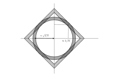
Figure 4: A cartoon view of the $\ell^{1}$ and $\ell^{2}$ “rings” where vectors with iid Laplace-distributed entries concentrate. The radius of the $\ell^{2}$ ring is of the order of $\sqrt{2/N}$ while that of the $\ell^{1}$ ring is one, corresponding to vectors with flat entries $|\mathbf{x}|_{n}\approx 1/N$.

Instead of model (24) we consider a more natural normalization of $\sigma_{k}(\mathbf{x})_{q}$ with respect to the size of the original vector $\mathbf{x}$ measured in the same norm. This is the best $k$-term relative error $\bar{\sigma}_{k}(\mathbf{x})_{q}$ that we investigated in Proposition 1. The class of vectors defined by $\bar{\sigma}_{k}(\mathbf{x})_{q}<C$ for some $C$ does not have the shape of an $\ell^{r}$ ball or weak $\ell^{r}$ ball. Instead it forms a set of compressible ‘rays’ as depicted in Figure 3 (b).

III-A Limits of G-CS guarantees using instance optimality

In terms of the relative best $k$-term approximation error, the instance optimality implies the following inequality:

$$\frac{\|\Delta(\mathbf{\Phi}\mathbf{x})-\mathbf{x}\|}{\|\mathbf{x}\|}\leq\min_{k}\left\{C_{k}\cdot\bar{\sigma}_{k}(\mathbf{x})\right\}$$

Note that if we have the following inequality satisfied for the particular realization of $\mathbf{x}$

$$\frac{\sigma_{k}(\mathbf{x})}{\|\mathbf{x}\|}\geq C_{k}^{-1},\forall k,$$

then the only consequence of instance optimality is that $\|\Delta(\mathbf{\Phi}\mathbf{x})-\mathbf{x}\|\leq\|\mathbf{x}\|$. In other words, the performance guarantee for the considered vector $\mathbf{x}$ is no better than for the trivial zero estimator: $\Delta_{\textrm{trivial}}(\mathbf{y})=0$, for any $\mathbf{y}$.

This simple observation illustrates that one should be careful in the interpretation of instance optimality. In particular, decoding algorithms with instance optimality guarantees may not universally perform better than other simple or more standard estimators.

To understand what this implies for specific distributions, consider the case of $\ell^{1}$ decoding with a Gaussian encoder $\Phi_{N}$. For this coder, decoder pair, $\{\Phi_{N},\Delta_{1}\}$, we know there is a strong phase transition associated with the robust null space property (20) with $0<\eta<1$ (and hence the instance optimality property with $1<C<\infty$) in terms of the undersampling factor $\delta:=m/N$ and the factor $\rho:=k/m$ as $k,m,N\rightarrow\infty$ [33]. This is a generalization of the $\ell^{1}$ exact recovery phase transition of Donoho and Tanner [16] which corresponds to $\eta=1$. We can therefore identify the smallest instance optimality constant asymptotically possible as a function of $\rho$ and $\delta$ which we will term $C(\rho,\delta)$.

To check whether instance optimality guarantees can beat the trivial zero estimator $\Delta_{\textrm{trivial}}$ for a given undersampling ratio $\delta$, and a given generative model $p(x)$, we need to consider the product of $\bar{\sigma}_{k}(\mathbf{x})_{1}\stackrel{{\scriptstyle a.s.}}{{\rightarrow}}G_{1}[p](\kappa)$ and $C(\frac{\kappa}{\delta},\delta)$. If

$$G_{1}[p](\kappa)>\frac{1}{C\left(\frac{\kappa}{\delta},\delta\right)},\quad\forall\kappa\in[0,\delta]$$ (25)

then the instance optimality offers no guarantee to outperform the trivial zero estimator.

In order to determine the actual strength of instance optimality we make the following observations:

• $C(\frac{\kappa}{\delta},\delta)\geq 2$ for all $\kappa$ and $\delta$;

• $C(\frac{\kappa}{\delta},\delta)=\infty$ for all $\delta$ if $\kappa>\kappa_{0}\approx 0.18$.

The first observation comes from minimising $C_{k}$ in (21) with respect to $0\leq\eta\leq 1$. The second observation stems from the fact that $\kappa_{0}:=\max_{\{\eta,\delta\}}\rho_{\eta}(\delta)\approx 0.18$ [16] (where $\rho_{\eta}(\delta)$ is the strong threshold associated to the null space property with constant $\eta\leq 1$) therefore we have $\kappa=\delta\rho\leq\kappa_{0}\approx 0.18$ for any finite $C$. From these observations we obtain :

For distributions with PDF $p(x)$ satisfying $G_{1}[p](\kappa_{0})\geq 1/2$, in high dimension $N$, instance optimality results for the decoder $\Delta_{1}$ with a Gaussian encoder can at best guarantee the performance (in the $\ell^{1}$ norm) of …the trivial decoder $\Delta_{\textrm{trivial}}$.

One might try to weaken the analysis by considering typical joint behavior of $\Phi_{N}$ and $\mathbf{x}_{N}$. This corresponds to the ‘weak’ phase transitions [16, 33]. For this scenario there is a modified $\ell^{1}$ instance optimality property [33], however the constant still satisfies $C(\frac{\kappa}{\delta},\delta)\geq 2$. Furthermore since $\kappa\leq\delta$ we can define an undersampling ratio $\delta_{0}$ by $G_{1}[p](\delta_{0})=1/2$, such that weak instance optimality provides no guarantee that $\Delta_{1}$ will outperform the trivial decoder $\Delta_{\textrm{trivial}}$ in the region $0<\delta\leq\delta_{0}$. More careful analysis will only increase the size of this region.

Example 3 (The Laplace distribution).

Suppose that $\mathbf{x}_{N}=(X_{1},\ldots,X_{N})$ has iid entries $X_{n}$ that follow the Laplace distribution with PDF $p_{1}(x)$. Then for large $N$, as noted in Example 1, the relative best $k$-term error is given by:

$$G_{1}[p_{1}](\kappa)=1-\kappa\cdot\Big{(}1+\ln 1/\kappa\Big{)}$$

Figure 5 shows that unfortunately this function exceeds $1/2$ on the interval $\kappa\in[0,\ \kappa_{0}]$ indicating there are no non-trivial performance guarantees from instance optimality. Even exploiting weak instance optimality we can have no non-trivial guarantees below $\delta_{0}\approx 0.18$.

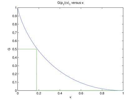
Figure 5: The $\ell^{1}$-norm best $k$-term approximation relative error $G_{1}[p_{1}](\kappa)$ as a function of $\kappa=k/N$ (top curve) along with a rectangular shaped function (bottom curve) that upper bounds $\inf_{\delta}C^{-1}(\kappa/\delta,\delta)$.

III-B CS guarantees for random variables with unbounded second moment

A more positive result (Theorem 2) can be obtained showing that random variables with infinite second moment, which are highly compressible (cf Proposition 1), are almost perfectly estimated by the $\ell^{1}$ decoder $\Delta_{1}$. In short, the result is based upon a variant of instance optimality: $\ell^{2}$ instance optimality in probability [13] which can be shown to hold for a large class of random matrices [15]. This can be combined with the fact that when $\mathbb{E}X^{2}=\infty$, from Proposition 1, we have $G_{2}[p](\kappa)=0$ for all $0<\kappa\leq 1$ to give Theorem 2. The proof is in the Appendix.

Remark 1.

A similar result can be derived based on $\ell^{1}$ instance optimality that shows that when $\mathbb{E}|X|=\infty$, then the relative error in $\ell^{1}$ for the $\ell^{1}$ decoder with a Gaussian encoder asymptotically goes to zero:

$$\lim_{N\to\infty}\frac{\|\Delta_{1}(\mathbf{\Phi}_{N}\mathbf{x}_{N})-\mathbf{x}_{N}\|_{1}}{\|\mathbf{x}_{N}\|_{1}}\stackrel{{\scriptstyle a.s.}}{{=}}0.$$

Whether other results hold for general $\ell^{p}$ decoders and relative $\ell^{p}$ error is not known.

We can therefore conclude that a random variable with infinite variance is not only compressible (in the sense of Proposition 1): it can also be accurately approximated from undersampled measurements within a compressive sensing scenario. In contrast, instance optimality provides no guarantees of compressibility when the variance is finite and $G_{1}[p](\kappa_{0})\geq 1/2$. At this juncture it is not clear where the blame for this result lies. Is it in the strength of the instance optimality theory, or are distributions with finite variance simply not able to generate sufficiently compressible vectors for sparse recovery to be successful at all? We will explore this latter question further in subsequent sections.

IV G-CS performance of oracle sparse reconstruction vs least squares

Consider $\mathbf{x}$ an arbitrary vector in $\mathbb{R}^{N}$ and $\mathbf{\Phi}$ be an $m\times N$ Gaussian encoder, and let $\mathbf{y}:=\mathbf{\Phi}\mathbf{x}$. Besides the trivial zero estimator $\Delta_{\textrm{trivial}}$ (14) and the $\ell^{1}$ minimization estimator $\Delta_{1}$ (11), the Least Squares (LS) estimator $\Delta_{\textrm{LS}}$ (12) is a commonly used alternative. Due to the Gaussianity of $\mathbf{\Phi}$ and its independence from $\mathbf{x}$, it is well known that the resulting relative expected performance is

$$\frac{\mathbb{E}_{\mathbf{\Phi}}\|\Delta_{\textrm{LS}}(\mathbf{\Phi}\mathbf{x})-\mathbf{x}\|_{2}^{2}}{\|\mathbf{x}\|_{2}^{2}}=1-\frac{m}{N}.$$ (26)

Moreover, there is indeed a concentration around the expected value, as expressed by the inequality below:

$$(1-\epsilon)\left(1-\frac{m}{N}\right)\leq\frac{\|\Delta_{\textrm{LS}}(\mathbf{\Phi}\mathbf{x})-\mathbf{x}\|_{2}^{2}}{\|\mathbf{x}\|_{2}^{2}}\leq(1-\epsilon)^{-1}\left(1-\frac{m}{N}\right),$$ (27)

for any $\epsilon>0$ and $\mathbf{x}\in\mathbb{R}^{N}$, except with probability at most $2\cdot e^{-(N-m)\epsilon^{2}/4}+2\cdot e^{-N\epsilon^{2}/4}$.

The result is independent of the vector $\mathbf{x}$, which should be no surprise since the Gaussian distribution is isotropic. The expected performance is directly governed by the undersampling factor, i.e. the ratio between the number of measures $m$ and the dimension $N$ of the vector $\mathbf{x}$, $\delta:=m/N$.

In order to understand which statistical PDFs $p(x)$ lead to “compressible enough” vectors $\mathbf{x}$, we wish to compare the performance of LS with that of estimators $\Delta$ that exploit the sparsity of $\mathbf{x}$ to estimate it. Instead of choosing a particular estimator (such as $\Delta_{1}$), we consider the oracle sparse estimator $\Delta_{\textrm{oracle}}$ defined in (13), which is likely to upper bound the performance of most sparsity based estimators. While in practice $\mathbf{x}$ must be estimated from $\mathbf{y}=\mathbf{\Phi}\mathbf{x}$, the oracle is given a precious side information: the index set $\Lambda$ associated to the $k$ largest components in $\mathbf{x}$, where $k<m$. Given this information, the oracle computes

$$\Delta_{\textrm{oracle}}(\mathbf{y},\Lambda):=\operatorname*{argmin}_{\textrm{support}(\mathbf{x})=\Lambda}\|\mathbf{y}-\mathbf{\Phi}\mathbf{x}\|_{2}^{2}=\mathbf{\Phi}_{\Lambda_{k}}^{+}\mathbf{y},$$

where, since $k<m$, the pseudo-inverse is $\mathbf{\Phi}_{\Lambda}^{+}=(\mathbf{\Phi}_{\Lambda}^{T}\mathbf{\Phi}_{\Lambda})^{-1}\mathbf{\Phi}_{\Lambda}^{T}$. Unlike LS, the expected performance of the oracle estimators drastically depend on the shape of the best $k$-term approximation relative error of $\mathbf{x}$. Denoting $\mathbf{x}_{I}$ the vector whose entries match those of $\mathbf{x}$ on an index set $I$ and are zero elsewhere, and $\bar{I}$ the complement of an index set, we have the following result.

Theorem 3 (Expected performance of oracle sparse estimation).

Let $\mathbf{x}\in\mathbb{R}^{N}$ be an arbitrary vector, $\mathbf{\Phi}$ be an $m\times N$ random Gaussian matrix, and $\mathbf{y}:=\mathbf{\Phi}\mathbf{x}$. Let $\Lambda$ be an index set of size $k<m-1$, either deterministic, or random but statistically independent from $\mathbf{\Phi}$. We have

$$\frac{\mathbb{E}_{\mathbf{\Phi}}\|\Delta_{\textrm{oracle}}(\mathbf{\Phi}\mathbf{x},\Lambda)-\mathbf{x}\|_{2}^{2}}{\|\mathbf{x}\|_{2}^{2}} =\frac{1}{1-\frac{k}{m-1}}\times\frac{\|\mathbf{x}_{\bar{\Lambda}}\|_{2}^{2}}{\|\mathbf{x}\|_{2}^{2}}$$

$$\geq\frac{1}{1-\frac{k}{m-1}}\times\frac{\sigma_{k}(\mathbf{x})_{2}^{2}}{\|\mathbf{x}\|_{2}^{2}}.$$ (28)

If $\Lambda$ is chosen to be the $k$ largest components of $\mathbf{x}$, then the last inequality is an equality. Moreover, we can characterize the concentration around the expected value as

$$1+\frac{k(1-\epsilon)^{3}}{m-k+1} \leq\frac{\|\Delta_{\textrm{oracle}}(\mathbf{\Phi}\mathbf{x},\Lambda)-\mathbf{x}\|_{2}^{2}}{\|\mathbf{x}_{\bar{\Lambda}}\|_{2}^{2}}\leq 1+\frac{k(1-\epsilon)^{-3}}{m-k+1}$$ (29)

except with probability at most

$$8\cdot e^{-\min(k,m-k+1)\cdot c_{l}(\epsilon)/2},$$ (30)

where

$$\ c_{l}(\epsilon) :=-\ln(1-\epsilon)-\epsilon\geq\epsilon^{2}/2.$$ (31)

Remark 2.

Note that this result assumes that $\Lambda$ is statistically independent from $\mathbf{\Phi}$. Interestingly, for practical decoders such as the $\ell^{1}$ decoder, $\Delta_{1}$, the selected $\Lambda$ might not satisfy this assumption, unless the decoder successfully identifies the support of the largest components of $\mathbf{x}$.

IV-A Compromise between approximation and conditioning

We observe that the expected performance of both $\Delta_{LS}$ and $\Delta_{\textrm{oracle}}$ is essentially governed by the quantities $\delta=m/N$ and $\rho=k/m$, which are reminiscent of the parameters in the phase transition diagrams of Donoho and Tanner [16]. However, while in the work of Donoho and Tanner the quantity $\rho$ parameterizes a model on the vector $\mathbf{x}_{N}$, which is assumed to be $\rho\delta N$-sparse, here $\rho$ rather indicates the order of $k$-term approximation of $\mathbf{x}_{N}$ that is chosen in the oracle estimator. In a sense, it is more related to a stopping criterion that one would use in a greedy algorithm. The quantity that actually models $\mathbf{x}_{N}$ is the function $G_{2}[p]$, provided that $\mathbf{x}_{N}\in\mathbb{R}^{N}$ has iid entries $X_{n}$ with PDF $p(x)$ and finite second moment $\mathbb{E}X^{2}<\infty$. Indeed, combining Proposition 1 and Theorem 3 we obtain:

Theorem 4.

Let $\mathbf{x}_{N}$ be iid with respect to $p(x)$ as in Proposition 1. Assume that $\mathbb{E}X^{2}<\infty$. Let $\phi_{i,j}$, $i,j\in\mathbb{N}$ be iid Gaussian variables $\mathcal{N}(0,1)$. Consider two sequences $k_{N},m_{N}$ of integers and assume that

$$\lim_{N\to\infty}k_{N}/m_{N}=\rho\quad\mbox{and}\quad\lim_{N\to\infty}m_{N}/N=\delta.$$ (32)

Define the $m_{N}\times N$ Gaussian encoder $\mathbf{\Phi}_{N}=\left[\phi_{ij}/\sqrt{m_{N}}\right]_{1\leq i\leq m_{N},1\leq j\leq N}$. Let $\Lambda_{N}$ be the index of the $k_{N}$ largest magnitude coordinates of $\mathbf{x}_{N}$. We have the almost sure convergence

$$\lim_{N\to\infty}\frac{\|\Delta_{\textrm{oracle}}(\mathbf{\Phi}_{N}\mathbf{x}_{N},\Lambda_{N})-\mathbf{x}_{N}\|_{2}^{2}}{\|\mathbf{x}_{N}\|_{2}^{2}} \stackrel{{\scriptstyle a.s.}}{{=}} \frac{G_{2}[p](\rho\delta)}{1-\rho};$$ (33)

$$\lim_{N\to\infty}\frac{\|\Delta_{\textrm{LS}}(\mathbf{\Phi}_{N}\mathbf{x}_{N})-\mathbf{x}_{N}\|_{2}^{2}}{\|\mathbf{x}_{N}\|_{2}^{2}} \stackrel{{\scriptstyle a.s.}}{{=}} 1-\delta.$$ (34)

For a given undersampling ratio $\delta=m/N$, the asymptotic expected performance of the oracle therefore depends on the relative number of components that are kept $\rho=k/m$, and we observe the same tradeoff as discussed in Section III:

• For large $k$, close to the number of measures $m$ ($\rho$ close to one), the ill-conditioning of the pseudo-inverse matrix $\mathbf{\Phi}_{\Lambda}$ (associated to the factor $1/(1-\rho)$) adversely impacts the expected performance;

• For smaller $k$, the pseudo-inversion of this matrix is better conditioned, but the $k$-term approximation error governed by $G_{2}[p](\rho\delta)$ is increased.

Overall, for some intermediate size $k\approx\rho^{\star}m$ of the oracle support set $\Lambda_{k}$, the best tradeoff between good approximation and good conditioning is achieved, leading at best to the asymptotic expected performance

$$H[p](\delta):=\inf_{\rho\in(0,1)}\frac{G_{2}[p](\rho\delta)}{1-\rho}.$$ (35)

V A comparison of least squares and oracle sparse methods

The question that we will now investigate is how the expected performance of oracle sparse methods compares to that of least squares, i.e., how large is $H[p](\delta)$ compared to $1-\delta$? We are particularly interested in understanding how they compare for small $\delta$. Indeed, large $\delta$ values are associated with scenarii that are quite irrelevant to, for example, compressive sensing since the projection $\mathbf{\Phi}\mathbf{x}$ cannot significantly compress the dimension of $\mathbf{x}$. Moreover, it is in the regime where $\delta$ is small that the expected performance of least squares is very poor, and we would like to understand for which PDFs $p$ sparse approximation is an inappropriate tool. The answer will of course depend on the PDF $p$ through the function $G[p](\cdot)$. To characterize this we will say that a PDF $p$ is incompressible at a subsampling rate of $\delta$ if

$$H[p](\delta)>1-\delta.$$

In practice, there is often a minimal undersampling rate, $\delta_{0}$, such that for $\delta\in(0,\delta_{0})$ least squares estimation dominates the oracle sparse estimator. Specifically we will show below that PDFs $p(x)$ with a finite fourth moment $\mathbb{E}X^{4}<\infty$, such as generalized Gaussians, always have some minimal undersampling rate $\delta_{0}\in(0,1)$ below which they are incompressible. As a result, unless we perform at least $m\geq\delta_{0}N$ random Gaussian measurement of an associated $\mathbf{x}_{N}$, it is not worth relying on sparse methods for reconstruction since least squares can do as good a job.

When the fourth moment of the distribution is infinite, one might hope that the converse is true, i.e. that no such minimal undersampling rate $\delta_{0}$ exists. However, this is not the case. We will show that there is a PDF $p_{0}$, with infinite fourth moment and finite second moment, such that

$$H[p_{0}](\delta)=1-\delta,\qquad\forall\delta\in(0,1).$$

Up to a scaling factor, this PDF is associated to the symmetric PDF

$$p_{0}(x):=\frac{2|x|}{(x^{2}+1)^{3}}$$ (36)

and illustrates that least squares can be competitive with oracle sparse reconstruction even when the fourth moment is infinite.

V-A Distributions incompatible with extreme undersampling

In this section we show that when a PDF $p(x)$ has a finite fourth moment, $\mathbb{E}X^{4}<\infty$, then it will generate vectors which are not sufficiently compressible to be compatible with compressive sensing at high level of undersampling. We begin by showing that the comparison of $H[p](\delta)$ to $1-\delta$ is related to that of $G_{2}[p](\kappa)$ with $(1-\sqrt{\kappa})^{2}$.

Lemma 1.

Consider a function $G(\kappa)$ defined on $(0,1)$ and define

$$H(\delta):=\inf_{\rho\in(0,1)}\frac{G(\delta\rho)}{1-\rho}.$$ (37)

1. If $G(\delta^{2})\leq(1-\delta)^{2}$,
   then $H(\delta)\leq 1-\delta$.

2. If $G(\kappa)\leq(1-\sqrt{\kappa})^{2}$ for all $\kappa\in(0,\sqrt{\delta_{0}})$,
   then $H(\delta)\leq 1-\delta$ for all $\delta\in(0,\delta_{0})$.

3. If $G(\kappa)\geq(1-\sqrt{\kappa})^{2}$ for all $\kappa\in(0,\delta_{0})$,
   then $H(\delta)\geq 1-\delta$ for all $\delta\in(0,\delta_{0})$.

Lemma 1 allows us to deal directly with $G_{2}[p](\kappa)$ instead of $H[p](\delta)$. Furthermore the $(1-\sqrt{\kappa})^{2}$ term can be related to the fourth moment of the distribution (see Lemma 3 in the Appendix) giving the following result, which implies Theorem 1:

Theorem 5.

If $\mathbb{E}_{p(x)}X^{4}<\infty$, then there exists a minimum undersampling $\delta_{0}=\delta_{0}[p]>0$ such that for $\delta<\delta_{0}$,

$$H[p](\delta)\geq 1-\delta,\forall\ \delta\in(0,\delta_{0}).$$ (38)

and the performance of the oracle $k$-sparse estimation as described in Theorem 4 is asymptotically almost surely worse than that of least squares estimation as $N\rightarrow\infty$.

Roughly speaking, if $p(x)$ has a finite fourth moment, then in the regime where the relative number of measurement is (too) small we obtain a better reconstruction with least squares than with the oracle sparse reconstruction!

Note that this is rather strong, since the oracle is allowed to know not only the support of the $k$ largest components of the unknown vector, but also the best choice of $k$ to balance approximation error against numerical conditioning. A striking example is the case of generalized Gaussian distributions discussed below.

One might also hope that, reciprocally, having an infinite fourth moment would suffice for a distribution to be compatible with compressed sensing at extreme levels of undersampling. The following result disproves this hope.

Proposition 2.

With the PDF $p_{0}(x)$ defined in (36), we have

$$H[p_{0}](\delta)=1-\delta,\forall\ \delta\in(0,1).$$ (39)

On reflection this should not be that surprising. The PDF $p_{0}(x)$ has no probability mass at $x=0$ and resembles a smoothed Bernoulli distribution with heavy tails.

V-B Worked example: the generalized Gaussian distributions

Theorem 5 applies in particular whenever $\mathbf{x}_{N}$ is drawn from a generalized Gaussian distribution,

$$p_{\tau}(x)\propto\exp\left(-c|x|^{\tau}\right),$$ (40)

where $0<\tau<\infty$. The shape parameter, $\tau$ controls how heavy or light the tails of the distribution are. When $\tau=2$ the distribution reduces to the standard Gaussian, while for $\tau<2$ it gives a family of heavy tailed distributions with positive kurtosis. When $\tau=1$ we have the Laplace distribution and for $\tau\leq 1$ it is often considered that the distribution is in some way “sparsity-promoting”. However, the generalized Gaussian always has a finite fourth moment for all $\tau>0$. Thus Theorem 5 informs us that for a given parameter $\tau$ there is always a critical undersampling value below which the generalized Gaussian is incompressible.

While Theorem 5 indicates the existence of a critical $\delta_{0}$ it does not provide us with a useful bound. Fortunately, although in general we are unable to derive explicit expressions for $G[p](\cdot)$ and $H[p](\delta)$ (with the exceptions of $\tau=1,2$ - see Appendix -I), the generalized Gaussian has a closed form expression for its cdf in terms of the incomplete gamma function.

$$F(x)=\frac{1}{2}+\operatorname*{sgn}(x)\frac{\gamma\left(1/\tau,c|x|^{\tau}\right)}{2\Gamma(1/\tau)}$$

where $\Gamma(\cdot)$ and $\gamma(\cdot,\cdot)$ are respectively the gamma function and the lower incomplete gamma function. We are therefore able to numerically compute the value of $\delta_{0}$ as a function of $\tau$ with relative ease. This is shown in Figure 6. We see that, unsurprisingly, when $\tau$ is around $2$ there is little to be gained even with an oracle sparse estimator over standard least squares estimation. When $\tau=1$ (Laplace distribution) the value of $\delta_{0}\approx 0.15$, indicating that when subsampling by a factor of roughly 7 the least squares estimator will be superior. At this level of undersampling the relative error is a very poor: $0.85$, that is a performance of $0.7$dB in terms of traditional Signal to Distortion Ratio (SDR).

The critical undersampling value steadily drops as $\tau$ tends towards zero and the distribution becomes increasingly leptokurtic. Thus data distributed according to the generalized Gaussian for small $\tau\ll 1$ may still be a reasonable candidate for compressive sensing distributions as long as the undersampling rate is kept significantly above the associated $\delta_{0}$.

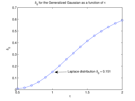
Figure 6: A plot of the critical subsampling rate, $\delta_{0}$ below which the generalized Gaussian distribution is incompressible as a function of the shape parameter, $\tau$.

V-C Expected Relative Error for the Laplace distribution

We conclude this section by examining in more detail the performance of the estimators for Laplace distributed data at various undersampling values. We have already seen from Figure 6 that the oracle performance is poor when subsampling by roughly a factor of 7. What about more modest subsampling factors? Figure 1 plots the relative error as a function of undersampling rate, $\delta$. The horizontal lines indicate SDR values of $3$dB, $10$dB and $20$dB. Thus for the oracle estimator to achieve 10dB the undersampling rate must be greater than 0.7, while to achieve a performance level of $20$dB, something that might reasonably be expected in many sensing applications, we can hardly afford any subsampling at all since this requires $\delta>0.9$.

At this point we should remind the reader that these performance results are for the comparison between the oracle sparse estimator and linear least squares. For practically implementable reconstruction algorithms we would expect that the critical undersampling rate at which least squares wins would be significantly higher. Indeed, as shown in Figure 1, this is what is empirically observed for the average performance of the $\ell^{1}$ estimator (11) applied to Laplace distributed data. This curve was calculated at various values of $\delta$ by averaging the relative error of 5000 $\ell^{1}$ reconstructions of independent Laplace distributed realizations of $\mathbf{x}_{N}$ with $N=256$. In particular note that the $\ell^{1}$ estimator only outperforms least squares for undersampling $\delta$ above approximately 0.65!

VI Concluding discussion

As we have just seen, Generalized Gaussian distributions are incompressible at low subsampling rates because their fourth moment is always finite. This confirms the results of Cevher obtained with a different approach [9], but may come as a surprise: for $0<\tau\leq 1$ the minimum $\ell^{\tau}$ norm solution to $\mathbf{y}=\mathbf{\Phi}\mathbf{x}$, which is also the MAP estimator under the Generalized Gaussian prior, is known to be a good estimator of $\mathbf{x}_{0}$ when $\mathbf{y}=\mathbf{\Phi}\mathbf{x}_{0}$ and $\mathbf{x}_{0}$ is compressible [14]. This highlights the need to distinguish between an estimator and its MAP interpretation. In contrast, we describe below a family of PDFs $p_{\tau,s}$ which, for certain values of the parameters $\tau,s$, combines:

• superior asymptotic almost sure performance of oracle sparse estimation over least squares reconstruction $\Delta_{\textrm{oracle}}$, even in the largely undersampled scenarios $\delta\to 0$;

• connections between oracle sparse estimation and MAP estimation.

Example 4.

For $0<\tau<\infty,\ 1<s<\infty$ consider the probability density function

$$p_{\tau,s}(x)\propto(1+|x|^{\tau})^{-s/\tau}.$$ (41)

1. When $1<s\leq 3$, the distribution is compressible.
   Since $\mathbb{E}_{p_{\tau,s}}X^{2}=\infty$, Theorem 2 is applicable: the $\ell^{1}$ decoder with a Gaussian encoder has ideal asymptotic performance, even at arbitrary small undersampling $\delta=m/N$;

2. When $3<s<5$, the distribution remains somewhat compressible.
   On the one hand $\mathbb{E}_{p_{\tau,s}}X^{2}<\infty$, on the other hand $\mathbb{E}_{p_{\tau,s}}X^{4}=\infty$.
   A detailed examination of the $G_{1}[p_{\tau,s}]$ function shows that there exists a relative number of measures $\delta_{0}(\tau,s)>0$ such that in the low measurement regime $\delta<\delta_{0}$, the asymptotic almost sure performance of oracle of $k$-sparse estimation, as described in Theorem 4, with the best choice of $k$, is better than that of least squares estimation:

   $$H[p_{\tau,s}](\delta)<1-\delta,\forall\delta\in(0,\delta_{0}).$$ (42)

3. When $s>5$, the distribution is incompressible.
   Since $\mathbb{E}_{p_{\tau,s}}X^{4}<\infty$, Theorem 1 is applicable: with a Gaussian encoder, there is an undersampling ratio $\delta_{0}$ such that whenever $\delta<\delta_{0}$, the asymptotic almost sure performance of oracle sparse estimation is worse than that of least-squares estimation;

Comparing Proposition 2 with the above Example 4, one observes that both the PDF $p_{0}(x)$ (Equation (36)) and the PDFs $p_{\tau,s}$, $3<s<5$ satisfy $\mathbb{E}_{p_{\tau,s}}X^{2}<\infty$ and $\mathbb{E}_{p_{\tau,s}}X^{4}=\infty$. Yet, while $p_{0}$ is essentially incompressible, the PDFs $p_{\tau,s}$ in this range are compressible. This indicates that, for distributions with finite second moment and infinite fourth moment, compressibility depends not only on the tail of the distribution but also on their mass around zero. However the precise dependency is currently unclear.

For $\tau=2$, the PDF $p_{2,s}$ is a Student-t distribution. For $\tau=1$, it is called a generalized Pareto distribution. These have been considered in [9, 2] as examples of “compressible” distributions, with the added condition that $s\leq 2$. Such a restriction results from the use of $\ell^{2}-\ell^{1}$ instance optimality in [9, 2], which implies that sufficient compressibility conditions can only be satisfied when $\mathbb{E}_{p}|X|=\infty$. Here instead we exploit $\ell^{2}-\ell^{2}$ instance optimality in probability, making it possible to obtain compressibility when $\mathbb{E}X^{2}=\infty$. In other words, [9, 2] provides sufficient conditions on a PDF $p$ to check its compressibility, but is inconclusive in characterizing their incompressibility.

The family of PDFs, $p_{\tau,s}$ in the range $0<\tau\leq 1$, can also be linked with a sparsity-inducing MAP estimate. Specifically for an observation $\mathbf{y}=\mathbf{\Phi}\mathbf{x}$ of a given vector $\mathbf{x}\in\mathbb{R}^{N}$, one can define the MAP estimate under the probabilistic model where all entries of $\mathbf{x}$ are considered as iid distributed according to $p_{\tau,s}$:

$$\Delta_{\textrm{MAP}}(\mathbf{y}):=\arg\max_{\mathbf{x}|\mathbf{\Phi}\mathbf{x}=\mathbf{y}}\prod_{n=1}^{N}p_{\tau,s}(x_{n})=\operatorname*{argmin}_{\mathbf{x}|\mathbf{\Phi}\mathbf{x}=\mathbf{y}}\sum_{n=1}^{N}f_{\tau}(|x_{n}|).$$

where for $t\in\mathbb{R}^{+}$ we define $f_{\tau}(t):=\log(1+t^{\tau})=a_{\tau,s}-b_{\tau,s}\log p_{\tau,s}(|t|)$. One can check that the function $f_{\tau}$ is associated to an admissible $f$-norm as described in [22, 23]: $f(0)=0$, $f(t)$ is non-decreasing, $f(t)/t$ is non-increasing (in addition, we have $f(t)\sim_{t\to 0}t^{\tau}$). Observing that the MAP estimate is a “minimum $f$-norm” solution to the linear problem $\mathbf{y}=\mathbf{\Phi}\mathbf{x}$, we can conclude that whenever $\mathbf{x}$ is a “sufficiently (exact) sparse” vector, we have in fact [22, 23] $\Delta_{\textrm{MAP}}(\mathbf{\Phi}\mathbf{x})=\mathbf{x}$, and $\Delta_{\textrm{MAP}}(\mathbf{\Phi}\mathbf{x})=\Delta_{1}(\mathbf{\Phi}\mathbf{x})$ is also the minimum $\ell^{1}$ norm solution to $\mathbf{y}=\mathbf{\Phi}\mathbf{x}$, which can in turn be “interpreted” as the MAP estimate under the iid Laplace model. However, unlike the Laplace interpretation of $\ell^{1}$ minimization, here Example 4 indicates that such densities are better aligned to sparse reconstruction techniques. Thus the MAP estimate interpretation here may be more valid.

It would be interesting to determine whether the MAP estimator $\Delta_{\textrm{MAP}}(\mathbf{\Phi}\mathbf{x})$ for such distributions is in some way close to optimal (i.e. close to the minimum mean squared error solution for $\mathbf{x}$). This would give such estimators a degree of legitimacy from a Bayesian perspective. However, we have not shown that the estimator $\Delta_{\textrm{MAP}}(\mathbf{\Phi}\mathbf{x})$ provides a good estimate for data that is distributed according to $p_{\tau,s}$ since, if $\mathbf{x}$ is a large dimensional typical instance with entries drawn iid from the PDF $p_{\tau,s}(x)$, it is typically not exactly sparse, hence the uniqueness results of [22, 23] do not directly apply. One would need to resort to a more detailed robustness analysis in the spirit of [21] to get more precise statements relating $\Delta_{\textrm{MAP}}(\mathbf{\Phi}\mathbf{x})$ to $\mathbf{x}$.

-A Proof of Proposition 1

To prove Proposition 1 we will rely on the following theorem [5][Theorem 2.2].

Theorem 6.

Suppose that $F_{Y}$ is a continuous and strictly increasing cumulative density function on $[a,b]$ where $0\leq a<b\leq\infty$, with $F_{Y}(a)=0$, $F_{Y}(b)=1$. For $\sigma\in(0,\mu)$ where $\mu=\int_{a}^{b}ydF_{Y}(y)$, let $\tau\in(a,b)$ be defined by the equation $\sigma=\int_{a}^{\tau}ydF_{Y}(y)$. Let $s_{1},s_{2},\ldots$ be a sequence such that $\lim_{N\to\infty}s_{N}/N=\sigma$, and let $Y_{1},Y_{2}\ldots$ be iid random variables with cumulative density function $F_{Y}$. Let $Y_{1,N}\leq\ldots\leq Y_{N,N}$ be the increasing order statistics of $Y_{1},\ldots,Y_{N}$ and let $L_{N}=L(N,s_{n})$ be defined as $L(N,s_{n}):=0$ if $Y_{1,N}>s_{N}$, otherwise:

$$L(N,s_{n}):=\max\left\{\ell\leq N,Y_{1,N}+\ldots+Y_{\ell,N}\leq s_{N}\right\};$$ (43)

Then

$$\lim_{N\to\infty}\frac{Y_{L_{N},N}}{N}\stackrel{{\scriptstyle a.s.}}{{=}}\tau,$$ (44)

$$\lim_{N\to\infty}\frac{L_{N}}{N}\stackrel{{\scriptstyle a.s.}}{{=}}F_{Y}(\tau),$$ (45)

$$\lim_{N\to\infty}\frac{\mathbb{E}(L_{N})}{N}=F_{Y}(\tau).$$ (46)

Proof:

We begin by the case where $\mathbb{E}|X|^{q}<\infty$. We consider random variables $X_{n}$ drawn according the PDF $p(x)$, and we define the iid non-negative random variables $Y_{n}=|X_{n}|^{q}$. They have the cumulative density function $F_{Y}(y)=\mathbb{P}(Y\leq y)=\mathbb{P}(|X|\leq y^{1/q})=\bar{F}(y^{1/q})$, and we have $\mu=\mathbb{E}Y=\mathbb{E}|X|^{q}=\int_{0}^{\infty}|x|^{q}d\bar{F}(x)\in(0,\infty)$. We define $\mathbf{x}_{N}=(X_{n})_{n=1}^{N}$, and we consider a sequence $k_{N}$ such that $\lim_{N\to\infty}k_{N}/N=\kappa\in(0,1)$. By the assumptions on $F_{Y}$ there is a unique $\tau_{0}\in(0,\infty)$ such that $\kappa=1-F_{Y}(\tau_{0})$, and we will prove that

$$\liminf_{N\to\infty}\frac{\sigma_{k_{N}}(\mathbf{x}_{N})_{q}^{q}}{N\mu} \stackrel{{\scriptstyle a.s.}}{{\geq}} \frac{\int_{0}^{\tau_{0}}ydF_{Y}(y)}{\mu},$$ (47)

$$\limsup_{N\to\infty}\frac{\sigma_{k_{N}}(\mathbf{x}_{N})_{q}^{q}}{N\mu} \stackrel{{\scriptstyle a.s.}}{{\leq}} \frac{\int_{0}^{\tau_{0}}ydF_{Y}(y)}{\mu}.$$ (48)

The proof of the two bounds is identical, hence we only detail the first one. Fix $0<\epsilon<\tau_{0}$ and define $\tau=\tau(\epsilon):=\tau_{0}-\epsilon$, $\sigma=\sigma(\epsilon):=\int_{0}^{\tau}ydF_{Y}(y)$, and $s_{N}=N\sigma$. Defining $L_{N}$ as in (43), we can apply Theorem 6 and obtain $\lim_{N\to\infty}\frac{L_{N}}{N}\stackrel{{\scriptstyle a.s.}}{{=}}F_{Y}(\tau)$. Since $\lim_{N\to\infty}\frac{k_{N}}{N}=1-F_{Y}(\tau_{0})$, it follows that

$$\lim_{N\to\infty}\frac{N-k_{N}}{L_{N}}\stackrel{{\scriptstyle a.s.}}{{=}}\frac{F_{Y}(\tau_{0})}{F_{Y}(\tau)}>1$$

where we used the fact that $F_{Y}$ is strictly increasing and $\tau<\tau_{0}$. In other words, almost surely, we have $N-k_{N}>L_{N}$ for all large enough $N$. Now remember that by definition

$$L_{N}=\max\left\{\ell\leq N,\sigma_{N-\ell}(\mathbf{x}_{N})_{q}^{q}\leq N\sigma\right\}.$$

As a result, almost surely, for all large enough $N$, we have

$$\sigma_{k_{N}}(\mathbf{x}_{N})_{q}^{q}=\sigma_{N-(N-k_{N})}(\mathbf{x}_{N})_{q}^{q}>N\sigma.$$

Now, by the strong law of large number, we also have

$$\lim_{N\to\infty}\frac{\|\mathbf{x}_{N}\|_{q}^{q}}{N\mu}\stackrel{{\scriptstyle a.s.}}{{=}}1,$$

hence we obtain

$$\liminf_{N\to\infty}\frac{\sigma_{k_{N}}(\mathbf{x}_{N})_{q}^{q}}{\|\mathbf{x}_{N}\|_{q}^{q}}\stackrel{{\scriptstyle a.s.}}{{\geq}}\frac{\sigma}{\mu}=\frac{\int_{0}^{\tau_{0}-\epsilon}ydF_{Y}(y)}{\mu}.$$

Since this holds for any $\epsilon>0$ and $F_{Y}$ is continuous, this implies (47). The other bound (48) is obtained similarly. Since the two match, we get

$$\lim_{N\to\infty}\frac{\sigma_{k_{N}}(\mathbf{x}_{N})_{q}^{q}}{\|\mathbf{x}_{N}\|_{q}^{q}}\stackrel{{\scriptstyle a.s.}}{{=}}\frac{\int_{0}^{\tau_{0}}ydF_{Y}(y)}{\mu}=\frac{\int_{0}^{\tau_{0}}ydF_{Y}(y)}{\int_{0}^{\infty}ydF_{Y}(y)}.$$

Since $\kappa=1-F_{Y}(\tau_{0})=1-\bar{F}(\tau_{0}^{1/q})$ we have $\tau_{0}=\left[\bar{F}^{-1}(1-\kappa)\right]^{q}$. Since $F_{Y}(y)=\bar{F}(y^{1/q})$ we have $dF_{Y}(y)=\frac{1}{q}y^{1/q-1}\bar{p}(y^{1/q})dy$. As a result

$$\frac{\int_{0}^{\tau_{0}}ydF_{Y}(y)}{\int_{0}^{\infty}ydF_{Y}(y)} = \frac{\int_{0}^{\left[\bar{F}^{-1}(1-\kappa)\right]^{q}}y^{1/q}\bar{p}(y^{1/q})dy}{\int_{0}^{\infty}y^{1/q}\bar{p}(y^{1/q})dy}$$

$$\stackrel{{\scriptstyle(a)}}{{=}} \frac{\int_{0}^{\bar{F}^{-1}(1-\kappa)}x\bar{p}(x)x^{q-1}dx}{\int_{0}^{\infty}x\bar{p}(x)x^{q-1}dx}$$

$$= \frac{\int_{0}^{\bar{F}^{-1}(1-\kappa)}x^{q}\bar{p}(x)dx}{\int_{0}^{\infty}x^{q}\bar{p}(x)dx}$$

where in (a) we used the change of variable $y=x^{q}$, $x=y^{1/q}$, $dy=qx^{q-1}dx$. We have proved the result for $0<\kappa<1$, and we let the reader check that minor modifications yield the results for $\kappa=0$ and $\kappa=1$.

Now we consider the case $\mathbb{E}|X|^{q}=+\infty$. The idea is to use a “saturated” version $\tilde{X}$ of the random variable $X$, such that $\mathbb{E}|\tilde{X}|^{q}<\infty$, so as to use the results proven just above.

One can easily build a family of smooth saturation functions $f_{\eta}:[0\ +\infty)\to[0\ 2\eta)$, $0<\eta<\infty$ with $f_{\eta}(t)=t$, for $t\in[0,\eta]$, $f_{\eta}(t)\leq t$, for $t>\eta$, and two additional properties:

1. each function $t\mapsto f_{\eta}(t)$ is bijective from $[0,\infty)$ onto $[0,2\eta)$, with $f^{\prime}_{\eta}(t)>0$ for all $t$;

2. each function $t\mapsto f_{\eta}(t)/t$ is monotonically decreasing;

Denoting $f_{\eta}(\mathbf{x}):=(f_{\eta}(x_{i}))_{i=1}^{N}$, by [23, Theorem 5], the first two properties ensure that for all $1\leq k\leq N$, $\mathbf{x}\in\mathbb{R}^{N}$, $0<\eta,q<\infty$ we have

$$\frac{\sigma_{k}(\mathbf{x})^{q}}{\|\mathbf{x}\|_{q}^{q}}\leq\frac{\sigma_{k}(f_{\eta}(\mathbf{x}))^{q}}{\|f_{\eta}(\mathbf{x})\|_{q}^{q}}.$$ (49)

Consider a fixed $\eta$ and the sequence of “saturated” random variables $\tilde{X}_{i}=f_{\eta}(|X_{i}|)$. They are iid with $\mathbb{E}|\tilde{X}|^{q}<\infty$. Moreover, the first property of $f_{\eta}$ above ensures that their cdf $t\mapsto\bar{F}_{\eta}(t):=\mathbb{P}(f_{\eta}(|X|)\leq t)$ is continuous and strictly increasing on $[0\ 2\eta]$, with $\bar{F}_{\eta}(0)=0$ and $\bar{F}_{\eta}(\infty)=1$. Hence, by the first part of Proposition 1 just proven above, we have

$$\lim_{N\to\infty}\frac{\sigma_{k_{N}}(f_{\eta}(\mathbf{x}_{N}))^{q}}{\|f_{\eta}(\mathbf{x}_{N})\|_{q}^{q}} \stackrel{{\scriptstyle a.s.}}{{=}}G_{q}[\bar{p}_{\eta}](\kappa)=\frac{\int_{0}^{\bar{F}_{\eta}^{-1}(1-\kappa)}x^{q}\bar{p}_{\eta}(x)dx}{\int_{0}^{\infty}x^{q}\bar{p}_{\eta}(x)dx}$$

$$\leq\frac{|\bar{F}_{\eta}^{-1}(1-\kappa)|^{q}}{\mathbb{E}|f_{\eta}(X)|^{q}}.$$ (50)

Since $f_{\eta}(t)\leq t$ for all $t$, we have $\bar{F}_{\eta}(t)=\mathbb{P}(f_{\eta}(|X|)\leq t)\geq\mathbb{P}(|X|\leq t)=\bar{F}(t)$ for all $t$, hence $\bar{F}_{\eta}^{-1}(1-\kappa)\leq\bar{F}^{-1}(1-\kappa)$. Moreover, since $f_{\eta}(t)=t$ for $0\leq t\leq\eta$, we obtain $\mathbb{E}|f_{\eta}(X)|^{q}\geq\int_{0}^{\eta}x^{q}\bar{F}(x)dx$. Combining  (49) and (-A) with the above observations we obtain for any $0<\eta<\infty$

$$\limsup_{N\to\infty}\frac{\sigma_{k_{N}}(\mathbf{x}_{N})^{q}}{\|\mathbf{x}_{N}\|_{q}^{q}}\leq\lim_{N\to\infty}\frac{\sigma_{k_{N}}(f_{\eta}(\mathbf{x}_{N}))^{q}}{\|f_{\eta}(\mathbf{x}_{N})\|_{q}^{q}}\stackrel{{\scriptstyle a.s.}}{{\leq}}\frac{|\bar{F}^{-1}(1-\kappa)|^{q}}{\int_{0}^{\eta}x^{q}\bar{p}(x)dx}.$$

Since $\mathbb{E}|X|^{q}=\int_{0}^{\infty}x^{q}\bar{p}(x)dx=\infty$, the infimum over $\eta$ of the right hand side is zero. ∎

Remark 3.

To further characterize the typical asymptotic behaviour of the relative error when $\mathbb{E}_{p}(|X|^{q})=\infty$ and $k_{N}/N\to 0$ appears to require a more detailed characterization of the probability density function, such as decay bounds on the tails of the distribution.

-B Proof of Theorem 2

The proof is based upon the following version of [15, Theorem $5.1$]:

Theorem 7 (DeVore et al. [15]).

Let $\mathbf{\Phi}(\omega)\in\mathbb{R}^{m\times N}$ be a random matrix whose entries are iid and drawn from ${\cal N}(0,1/m)$. There are some absolute constants $C_{0},\ldots,C_{6}$, and $C_{7}$ depending on $C_{1},\ldots,C_{6}$ such that, given any $k\leq C_{0}m/\log(N/m)$ then

$$\|\mathbf{x}-\Delta_{1}(\mathbf{\Phi}(\omega)\mathbf{x})\|_{2}\leq C_{7}\sigma_{k}(\mathbf{x})_{2},$$ (51)

with probability exceeding

$$1-C_{1}e^{-C_{2}m}-e^{-C_{3}\sqrt{Nm}}-C_{4}e^{-C_{5}m}-2me^{-\frac{\sqrt{m}}{C_{6}\log(N/m)}}.$$

In this version of the theorem we have specialized to the case where the random matrices are Gaussian distributed. We have also removed the rather peculiar requirement in the original version that $N\geq[\ln 6]^{2}m$ as careful scrutiny of the proofs (in particular the proof of Theorem 3.5 [15]) indicates that the effect of this term can be absorbed into the constant $C_{3}$ as long as $m/N\leq[\tfrac{2}{\ln 6}]^{2}\approx 1.2$, which is trivially satisfied.

We now proceed to prove Theorem 2. By assumption the undersampling ratio $\delta=\lim_{N\rightarrow\infty}\tfrac{m_{N}}{N}>0$, therefore there exists a $0<\kappa<1$ such that

$$\delta>C_{0}\kappa\log\frac{1}{\delta}.$$

Now choosing a sequence $k_{N}/N\rightarrow\kappa$ we have, for large enough $N$,

$$m_{N} \geq C_{0}k_{N}\log(N/m_{N}).$$

Hence, applying Theorem 7, for all $N$ large enough, there exist a set $\Omega_{N}(\mathbf{x}_{N},k_{N})$ with

$$\mathbb{P}(\Omega_{N}^{c}(\mathbf{x}_{N},k_{N}))\leq C_{8}me^{-C_{9}\sqrt{m}}$$ (52)

such that (51) holds for all $\mathbf{\Phi}_{N}(\omega)\in\Omega(\mathbf{x}_{N},k_{N})$, i.e.,

$$\frac{\|\mathbf{x}_{N}-\Delta_{1}(\Phi_{N}(\omega)\mathbf{x}_{N})\|_{2}}{\|\mathbf{x}_{N}\|_{2}}\leq C_{7}\bar{\sigma}_{k_{N}}(\mathbf{x}_{N})_{2}.$$ (53)

A union bound argument similar to the one used in the proof of Theorem 4 (see Appendix -D) gives:

$$\limsup_{N\rightarrow\infty}\frac{\|\mathbf{x}_{N}-\Delta_{1}(\Phi_{N}\mathbf{x}_{N})\|_{2}}{\|\mathbf{x}_{N}\|_{2}} \stackrel{{\scriptstyle a.s.}}{{\leq}}\limsup_{N\rightarrow\infty}C_{7}\bar{\sigma}_{k_{N}}(\mathbf{x}_{N})_{2}$$

$$\stackrel{{\scriptstyle a.s.}}{{=}}C_{7}G_{2}[p](\kappa)=0.$$ (54)

-C Proof of Theorem 3

We will need concentration bounds for several distributions. For the Chi-square distribution with $n$ degrees of freedom $\chi^{2}_{n}$, we will use the following standard result (see, e.g., [3, Proposition 2.2], and the intermediate estimates in the proof of [3, Corollary 2.3]):

Proposition 3.

Let $X\in\mathbb{R}^{n}$ a standard Gaussian random variable. Then, for any $0<\epsilon<1$

$$\mathbb{P}\big{(}\|X\|_{2}^{2}\geq n(1-\epsilon)^{-1}\big{)} \leq e^{-n\cdot c_{u}(\epsilon)/2}$$ (55)

$$\mathbb{P}\big{(}\|X\|_{2}^{2}\leq n(1-\epsilon)\big{)}\leq e^{-n\cdot c_{l}(\epsilon)/2}$$ (56)

with

$$c_{u}(\epsilon) :=\frac{\epsilon}{1-\epsilon}+\ln(1-\epsilon)$$ (57)

$$c_{l}(\epsilon) :=-\ln(1-\epsilon)-\epsilon.$$ (58)

Note that

$$\epsilon^{2}/2\leq c_{l}(\epsilon)\leq c_{u}(\epsilon),\quad 0<\epsilon<1.$$ (59)

Its corollary, which provides concentration for projections of random variables from the unit sphere, will also be useful. The statement is obtained by adjusting [3, Lemma 3.2] and [3, Corollary 3.4] keeping the sharper estimate from above.

Corollary 1.

Let $X$ be a random vector uniformly distributed on the unit sphere in $\mathbb{R}^{n}$, and let $X_{L}$ be its orthogonal projection on a $k$-dimensional subspace $L$ (alternatively, let $X$ be an arbitrary random vector and $L$ be a random $k$-dimensional subspace uniformly distributed on the Grassmannian manifold). For any $0<\epsilon<1$ we have

$$\mathbb{P}\big{(}\sqrt{\frac{n}{k}}\|X_{L}\|_{2}\geq\|X\|_{2}(1-\epsilon)^{-1}\big{)}\leq e^{-k\cdot c_{u}(\epsilon)/2}+e^{-n\cdot c_{l}(\epsilon)/2},$$ (60)

$$\mathbb{P}\big{(}\sqrt{\frac{n}{k}}\|X_{L}\|_{2}\leq\|X\|_{2}(1-\epsilon)\big{)}\leq e^{-k\cdot c_{l}(\epsilon)/2}+e^{-n\cdot c_{u}(\epsilon)/2}.$$ (61)

The above result directly implies the concentration inequality (27) for the LS estimator mentioned in Section IV. We will also need a result about Wishart matrices. The Wishart distribution [25] $\mathcal{W}_{\ell}(n,\Sigma)$ is the distribution of $\ell\times\ell$ matrices $A=Z^{T}Z$ where $Z$ is an $n\times\ell$ matrix whose columns have the normal distribution $\mathcal{N}(0,\Sigma)$.

Theorem 8 ([25] [Theorem 3.2.12 and consequence, p. 97-98]).

If $A$ is $\mathcal{W}_{\ell}(n,\Sigma)$ where $n-\ell+1>0$, and if $Z\in\mathbb{R}^{\ell}$ is a random vector distributed independently of $A$ and with $P(Z=0)=0$, then the ratio $Z^{T}\Sigma^{-1}Z/Z^{T}A^{-1}Z$ follows a Chi-square distribution with $n-\ell+1$ degrees of freedom $\chi^{2}_{n-\ell+1}$, and is independent of $Z$. Moreover, if $n-\ell-1>0$ then

$$\mathbb{E}A^{-1}=\Sigma^{-1}\cdot(n-\ell-1)^{-1}.$$ (62)

Finally, for convenience we formalize below some useful but simple facts that we let the reader check.

Lemma 2.

Let $\mathbf{A}$ and $\mathbf{B}$ be two independent $m\times k$ and $m\times\ell$ random Gaussian matrices with iid entries $\mathcal{N}(0,1/m)$, and let $x\in\mathbb{R}^{\ell}$ be a random vector independent from $\mathbf{B}$. Consider a singular value decomposition (SVD) $\mathbf{A}=U\Sigma V$ and let $u_{\ell}$ be the columns of $U$. Define $w:=\mathbf{B}x/\|\mathbf{B}x\|_{2}\in\mathbb{R}^{m}$, $w_{1}:=(\langle u_{\ell},w\rangle)_{\ell=1}^{k}\in\mathbb{R}^{k}$, $w_{2}:=w_{1}/\|w_{1}\|_{2}\in\mathbb{R}^{k}$ and $w_{3}:=V^{T}w_{2}\in\mathbb{R}^{k}$. We have

1. $w$ is uniformly distributed on the sphere in $\mathbb{R}^{m}$, and statistically independent from $\mathbf{A}$;

2. the distribution of $w_{1}$ is rotationally invariant in $\mathbb{R}^{k}$, and it is statistically independent from $\mathbf{A}$;

3. $w_{2}$ is uniformly distributed on the sphere in $\mathbb{R}^{k}$, and statistically independent from $\mathbf{A}$;

4. $w_{3}$ is uniformly distributed on the sphere in $\mathbb{R}^{k}$, and statistically independent from $\mathbf{A}$.

We can now start the proof of Theorem 3. For any index set $J$, we denote $\mathbf{x}_{J}$ the vector which is zero out of $J$. For matrices, the notation $\mathbf{\Phi}_{J}$ indicates the sub-matrix of $\mathbf{\Phi}$ made of the columns indexed by $J$. The notation $\bar{J}$ stands for the complement of the set $J$. For any index set $\Lambda$ associated to linearly independent columns of $\mathbf{\Phi}_{\Lambda}$ we can write $\mathbf{y}=\mathbf{\Phi}_{\Lambda}\mathbf{x}_{\Lambda}+\mathbf{\Phi}_{\bar{\Lambda}}\mathbf{x}_{\bar{\Lambda}}$ hence

$$\Delta_{\textrm{oracle}}(\mathbf{y},\Lambda) := \mathbf{\Phi}_{\Lambda}^{+}\mathbf{y}=\mathbf{x}_{\Lambda}+\mathbf{\Phi}_{\Lambda}^{+}\mathbf{\Phi}_{\bar{\Lambda}}\mathbf{x}_{\bar{\Lambda}}$$

$$\|\Delta_{\textrm{oracle}}(\mathbf{y},\Lambda)-\mathbf{x}\|_{2}^{2} = \|\mathbf{\Phi}_{\Lambda}^{+}\mathbf{\Phi}_{\bar{\Lambda}}\mathbf{x}_{\bar{\Lambda}}\|_{2}^{2}+\|\mathbf{x}_{\bar{\Lambda}}\|_{2}^{2}$$ (63)

The last equality comes from the fact that the restriction of $(\Delta_{\textrm{oracle}}(\mathbf{y},\Lambda)-\mathbf{x})$ to the indices in $\Lambda$ is $\mathbf{\Phi}_{\Lambda}^{+}\mathbf{\Phi}_{\bar{\Lambda}}\mathbf{x}_{\bar{\Lambda}}$, while its restriction to $\bar{\Lambda}$ is $\mathbf{x}_{\bar{\Lambda}}$. Denoting

$$w:=\frac{\mathbf{\Phi}_{\bar{\Lambda}}\mathbf{x}_{\bar{\Lambda}}}{\|\mathbf{\Phi}_{\bar{\Lambda}}\mathbf{x}_{\bar{\Lambda}}\|_{2}}\in\mathbb{R}^{m}$$ (64)

we obtain the relation

$$\frac{\|\Delta_{\textrm{oracle}}(\mathbf{y},\Lambda)-\mathbf{x}\|_{2}^{2}}{\|\mathbf{x}_{\bar{\Lambda}}\|_{2}^{2}}=\underbrace{\|\mathbf{\Phi}_{\Lambda}^{+}w\|_{2}^{2}}_{A}\times\underbrace{\frac{\|\mathbf{\Phi}_{\bar{\Lambda}}\mathbf{x}_{\bar{\Lambda}}\|_{2}^{2}}{\|\mathbf{x}_{\bar{\Lambda}}\|_{2}^{2}}}_{B}+1.$$ (65)

From the singular value decomposition

$$\mathbf{\Phi}_{\Lambda}=U_{m}\cdot\left[\begin{array}[]{c}\Sigma_{k}\\ 0_{(m-k)\times k}\end{array}\right]\cdot V_{k},$$

where $U_{m}$ is an $m\times m$ unitary matrix with columns $u_{\ell}$, and $V_{k}$ is a $k\times k$ unitary matrix, we deduce that $\mathbf{\Phi}_{\Lambda}^{+}=V_{k}^{T}[\Sigma_{k}^{-1},0_{k\times(m-k)}]U_{m}^{T}$ and

$$\|\mathbf{\Phi}_{\Lambda}^{+}w\|_{2}^{2}=\|[\Sigma_{k}^{-1}0_{k\times(m-k)}]U_{m}^{T}w\|_{2}^{2}=\sum_{\ell=1}^{k}\sigma_{\ell}^{-2}|\langle u_{\ell},w\rangle|^{2}.$$ (66)

Since $\mathbf{\Phi}_{\bar{\Lambda}}$ and $\mathbf{x}_{\bar{\Lambda}}$ are statistically independent, the random vector $\mathbf{\Phi}_{\bar{\Lambda}}\mathbf{x}_{\bar{\Lambda}}\in\mathbb{R}^{m}$ is Gaussian with zero-mean and covariance $m^{-1}\cdot\|\mathbf{x}_{\bar{\Lambda}}\|_{2}^{2}\cdot\mathbf{Id}_{m}$. Therefore,

$$\mathbb{E}\left\{\|\mathbf{\Phi}_{\bar{\Lambda}}\mathbf{x}_{\bar{\Lambda}}\|_{2}^{2}/\|\mathbf{x}_{\bar{\Lambda}}\|_{2}^{2}\right\}=1$$ (67)

and by Proposition 3, for any $0<\epsilon_{0}<1$

$$\mathbb{P}\left(1-\epsilon_{0}\leq\frac{\|\mathbf{\Phi}_{\bar{\Lambda}}\mathbf{x}_{\bar{\Lambda}}\|_{2}^{2}}{\|\mathbf{x}_{\bar{\Lambda}}\|_{2}^{2}}\leq(1-\epsilon_{0})^{-1}\right)\geq 1-2\cdot e^{-m\cdot c_{l}(\epsilon_{0})/2}.$$ (68)

Moreover, by Lemma 2-item 2, the random variables $\langle u_{\ell},w\rangle$, $1\leq\ell\leq k$ are identically distributed and independent from the random singular values $\sigma_{\ell}$. Therefore,

$$\mathbb{E}\|\mathbf{\Phi}_{\Lambda}^{+}w\|_{2}^{2}= \mathbb{E}\left\{\sum_{\ell=1}^{k}\sigma_{\ell}^{-2}\right\}\times\mathbb{E}\{|\langle u,w\rangle|^{2}\}$$

$$= \mathbb{E}\left\{\text{Trace}(\mathbf{\Phi}_{\Lambda}^{T}\mathbf{\Phi}_{\Lambda})^{-1}\right\}\times\frac{1}{m}.$$

The matrix $\mathbf{\Phi}_{\Lambda}^{T}\mathbf{\Phi}_{\Lambda}$ is $\mathcal{W}_{k}(m,\frac{1}{m}\mathbf{Id}_{k})$ hence, by Theorem 8, when $m-k-1>0$ we have

$$\mathbb{E}\|\mathbf{\Phi}_{\Lambda}^{+}w\|_{2}^{2}=\frac{\operatorname{Trace}(m\mathbf{Id}_{k})}{(m-k-1)m}=\frac{k}{m-k-1}.$$ (69)

Now, considering $w_{1}:=(\langle u_{\ell},w\rangle)_{\ell=1}^{k}\in\mathbb{R}^{k}$, $w_{2}:=w_{1}/\|w_{1}\|_{2}$ and $w_{3}:=V_{k}^{T}w_{2}$, we obtain

$$\|\mathbf{\Phi}^{+}w\|_{2}^{2} =\|\Sigma_{k}^{-1}w_{1}\|_{2}^{2}=\|w_{1}\|_{2}^{2}\times\|\Sigma_{k}^{-1}w_{2}\|_{2}^{2}$$

$$=\|w_{1}\|_{2}^{2}\times\|\Sigma_{k}^{-1}V_{k}w_{3}\|_{2}^{2}$$

$$=\|w_{1}\|_{2}^{2}\times w_{3}^{T}(\mathbf{\Phi}_{\Lambda}^{T}\mathbf{\Phi}_{\Lambda})^{-1}w_{3}=m\|w_{1}\|_{2}^{2}/R(w_{3}),$$

where $R(w_{3}):=m\|w_{3}\|_{2}^{2}/w_{3}^{T}(\mathbf{\Phi}_{\Lambda}^{T}\mathbf{\Phi}_{\Lambda})^{-1}w_{3}=w_{3}^{T}(m^{-1}\mathbf{Id}_{k})^{-1}w_{3}/w_{3}^{T}(\mathbf{\Phi}_{\Lambda}^{T}\mathbf{\Phi}_{\Lambda})^{-1}w_{3}$. By Lemma 2-item 4, $w_{3}$ is statistically independent from $\mathbf{\Phi}_{\Lambda}$. As a result, by Theorem 8, the random variable $R(w_{3})$ follows a Chi-square distribution with $m-k+1$ degrees of freedom $\chi^{2}_{m-k+1}$, and by Proposition 3, for any $0<\epsilon_{1}<1$,

$$\mathbb{P} \Big{(}1-\epsilon_{1}\leq R(w_{3})^{-1}\cdot(m-k+1)\leq(1-\epsilon_{1})^{-1}\Big{)}$$

$$\geq 1-2e^{-(m-k+1)\cdot c_{l}(\epsilon_{1})/2}.$$ (70)

Moreover, since $$w_{1} k w 0<\epsilon_{2}<1$$ is a random -dimensional orthogonal projection of the unit vector , by Corollary 1, for any

$$\mathbb{P} \Big{(}1-\epsilon_{2}\leq m\|w_{1}\|_{2}^{2}/k\leq(1-\epsilon_{2})^{-1}\Big{)}$$

$$\geq 1-4e^{-k\cdot c_{l}(\epsilon_{2})/2}.$$ (71)

To conclude, since $\mathbf{\Phi}_{\bar{\Lambda}}\mathbf{x}_{\bar{\Lambda}}$ is Gaussian, its $\ell^{2}$-norm $\|\mathbf{\Phi}_{\bar{\Lambda}}\mathbf{x}_{\bar{\Lambda}}\|_{2}^{2}$ and direction $w$ are mutually independent, hence $\|\mathbf{\Phi}_{\Lambda}^{+}w\|_{2}^{2}$ and $\|\mathbf{\Phi}_{\bar{\Lambda}}\mathbf{x}_{\bar{\Lambda}}\|_{2}^{2}$ are also mutually independent. Therefore, we can combine the decomposition (65) with the expected values (67) and (69) to obtain

$$\frac{\mathbb{E}\|\Delta_{\textrm{oracle}}(\mathbf{y},\Lambda)-\mathbf{x}\|_{2}^{2}}{\|\mathbf{x}_{\bar{\Lambda}}\|_{2}^{2}} =\mathbb{E}\|\mathbf{\Phi}_{\Lambda}^{+}w\|_{2}^{2}\times\frac{\mathbb{E}\|\mathbf{\Phi}_{\bar{\Lambda}}\mathbf{x}_{\bar{\Lambda}}\|_{2}^{2}}{\|\mathbf{x}_{\bar{\Lambda}}\|_{2}^{2}}+1$$

$$=\frac{k}{m-k-1}+1=\frac{1}{1-\frac{k}{m-1}}.$$

We conclude that: for any index set $$\Lambda k k<m-1$$ of size at most , with , in expectation

$$\frac{\mathbb{E}\|\Delta_{\textrm{oracle}}(\mathbf{y},\Lambda)-\mathbf{x}\|_{2}^{2}}{\|\mathbf{x}\|_{2}^{2}} =\frac{\mathbb{E}\|\Delta_{\textrm{oracle}}(\mathbf{y},\Lambda)-\mathbf{x}\|_{2}^{2}}{\|\mathbf{x}_{\bar{\Lambda}}\|_{2}^{2}}\times\frac{\|\mathbf{x}_{\bar{\Lambda}}\|_{2}^{2}}{\|\mathbf{x}\|_{2}^{2}}$$

$$=\frac{1}{1-\frac{k}{m-1}}\times\frac{\|\mathbf{x}_{\bar{\Lambda}}\|_{2}^{2}}{\|\mathbf{x}\|_{2}^{2}}$$

$$\geq\frac{1}{1-\frac{k}{m-1}}\times\frac{\sigma_{k}(\mathbf{x})_{2}^{2}}{\|\mathbf{x}\|_{2}^{2}}.$$

In terms of concentration, combining (68), (-C), and (-C), we get that for $0<\epsilon_{0},\epsilon_{1},\epsilon_{2}<1$:

$$(1-\epsilon_{0})(1-\epsilon_{1})(1-\epsilon_{2})\leq \|\mathbf{\Phi}^{+}_{\Lambda}w\|_{2}^{2}\frac{\|\mathbf{\Phi}_{\bar{\Lambda}}\mathbf{x}_{\bar{\Lambda}}\|_{2}^{2}}{\|\mathbf{x}_{\bar{\Lambda}}\|_{2}^{2}}\frac{m-k+1}{k}$$

$$\leq[(1-\epsilon_{0})(1-\epsilon_{1})(1-\epsilon_{2})]^{-1}$$

except with probability at most (setting $\epsilon_{i}=\epsilon$, $i=0,1,2$)

$$2\cdot e^{-m\cdot c_{l}(\epsilon_{0})/2}+4\cdot e^{-k\cdot c_{l}(\epsilon_{2})/2}+2\cdot e^{-(m-k+1)\cdot c_{l}(\epsilon_{1})/2}$$

$$\leq 8\cdot e^{-\min(k,m-k+1)\cdot c_{l}(\epsilon)/2}.$$

-D Proof of Theorem 4

Remember that we are considering sequences $k_{N},m_{N},\mathbf{\Phi}_{N},\Lambda_{N},\mathbf{x}_{N}$. Denoting $\rho_{N}=k_{N}/m_{N}$ and $\delta_{N}=m_{N}/N$, we observe that the probability (29) can be expressed as $1-8e^{-N\cdot c_{N}(\epsilon)/2}$ where $c_{N}(\epsilon)=c_{l}(\epsilon)\cdot\delta_{N}\cdot\min(\rho_{N},1-\rho_{N})$. For any choice of $\epsilon$, we have

$$\lim_{N\to\infty}c_{N}(\epsilon)=c_{l}(\epsilon)\cdot\delta\cdot\min(\rho,1-\rho)>0,$$

hence $\sum_{N}e^{-N\cdot c_{N}(\epsilon)/2}<\infty$ and we obtain that for any $\eta>0$

$$\sum_{N}\mathbb{P}\left(\left|\left(\textstyle\frac{\|\Delta_{\textrm{oracle}}(\mathbf{y}_{N},\Lambda_{N})-\mathbf{x}_{N}\|_{2}^{2}}{\sigma_{k_{N}}(\mathbf{x}_{N})_{2}^{2}}-1\right)\times\textstyle\frac{m_{N}-k_{N}+1}{k_{N}}-1\right|\geq\eta\right)<\infty.$$

This implies [19, Corollary 4.6.1] the almost sure convergence

$$\lim_{N\to\infty}\left(\left(\frac{\|\Delta_{\textrm{oracle}}(\mathbf{y}_{N},\Lambda_{N})-\mathbf{x}_{N}\|_{2}^{2}}{\sigma_{k_{N}}(\mathbf{x}_{N})_{2}^{2}}-1\right)\times\frac{m_{N}-k_{N}+1}{k_{N}}\right)\stackrel{{\scriptstyle a.s.}}{{=}}1.$$

Finally, since $k_{N}/m_{N}=\rho_{N}\to\rho$ and $\delta_{N}\to\delta$, we also have

$$\lim_{N\to\infty}\frac{k_{N}}{m_{N}-k_{N}+1}=\frac{\rho}{1-\rho}$$

and we conclude that

$$\lim_{N\to\infty}\frac{\|\Delta_{\textrm{oracle}}(\mathbf{y}_{N},\Lambda_{N})-\mathbf{x}_{N}\|_{2}^{2}}{\|\mathbf{x}_{N}\|_{2}^{2}} \stackrel{{\scriptstyle a.s.}}{{=}}\frac{1}{1-\rho}\lim_{N\to\infty}\frac{\sigma_{k_{N}}(\mathbf{x}_{N})_{2}^{2}}{\|\mathbf{x}_{N}\|_{2}^{2}}$$

$$\stackrel{{\scriptstyle a.s.}}{{=}}\frac{G_{2}[{p}](\delta\rho)}{1-\rho}.$$

We obtain the result for the least squares decoder by copying the above arguments and starting from (27).

-E Proof of Lemma 1

For the first result we assume that $G(\delta^{2})\leq(1-\delta)^{2}$. We take $\rho=\delta$ and obtain by definition

$$H(\delta)\leq\frac{G(\delta\rho)}{1-\rho}=\frac{G(\delta^{2})}{1-\delta}\leq(1-\delta).$$

The second result is a straightforward consequence of the first one. For the last one, we consider $\delta\in(0,\delta_{0})$. For any $\rho\in(0,1)$ we set $\kappa:=\delta\rho\in(0,\delta_{0})$. Since for any pair $a,b\in(0,1)$ we have $(1-a)(1-b)\leq(1-\sqrt{ab})^{2}$, we have

$$G(\kappa)\geq(1-\sqrt{\kappa})^{2}\geq(1-\delta)(1-\rho)$$

and we conclude that

$$\forall\ \rho\in(0,1),\ \frac{G(\delta\rho)}{1-\rho}\geq 1-\delta.$$

-F Proof of Theorem 1 and Theorem 5

Theorem 1 and Theorem 5 can be proved from Theorem 4 and Lemma 1 along with the following result.

Lemma 3.

Let $p(x)$ be teh PDF of a distribution with finite fourth moment $\mathbb{E}X^{4}<\infty$. Then there exists some $\delta_{0}\in(0,1)$ such that the function $G_{2}[p](\kappa)$ as defined in Proposition 1 satisfies

$$G_{2}[p](\kappa)\geq(1-\sqrt{\kappa})^{2},\qquad\forall\kappa\in(0,\delta_{0}).\$$ (72)

Proof:

Without loss of generality we can assume that $p(x)$ has unit second moment, hence

$$G_{2}[p](\kappa):=\frac{\int_{0}^{\bar{F}^{-1}(1-\kappa)}u^{2}\bar{p}(u)du}{\int_{0}^{\infty}u^{2}\bar{p}(u)du}=1-\int_{\alpha}^{\infty}u^{2}\bar{p}(u)du,$$

where we denote $\alpha=\bar{F}^{-1}(1-\kappa)$, which is equivalent to $\kappa=1-\bar{F}(\alpha)=\int_{\alpha}^{\infty}\bar{p}(u)du$. The inequality $G_{2}[p](\kappa)\geq(1-\sqrt{\kappa})^{2}$ is equivalent to $2\sqrt{\kappa}\geq 1+\kappa-G_{2}[p](\kappa)$, that is to say

$$2\sqrt{\int_{\alpha}^{\infty}\bar{p}(u)du}\geq\int_{\alpha}^{\infty}(u^{2}+1)\bar{p}(u)du$$ (73)

By the Cauchy-Schwarz inequality

$$\int_{\alpha}^{\infty}(u^{2}+1)\bar{p}(u)du\leq\sqrt{\int_{\alpha}^{\infty}(u^{2}+1)^{2}\bar{p}(u)du}\cdot\sqrt{\int_{\alpha}^{\infty}\bar{p}(u)du}.$$

Since $\mathbb{E}X^{4}<\infty$, for all small enough $\kappa$ (i.e., large enough $\alpha$), the right hand side is arbitrarily smaller than $2\sqrt{\int_{\alpha}^{\infty}\bar{p}(u)du}$ hence the inequality $G_{2}[p](\kappa)\geq(1-\sqrt{\kappa})^{2}$ holds true. ∎

Proof:

Theorem 1 and Theorem 5 now follow by combining Lemma 3 and Lemma 1 to show that for a distribution with finite fourth moment there exists a $\delta_{0}\in(0,1)$ such that $H(\delta)\geq 1-\delta$ for all $\delta\in(0,\delta_{0})$. The asymptotic almost sure comparative performance of the estimators then follows from the concentration bounds in Theorem 3 and for the least squares estimator. ∎

-G Proof of Proposition 2

Just as in the proof of Lemma 3 above, we denote $\alpha=\bar{F}^{-1}(1-\kappa)$, which is equivalent to $\kappa=1-\bar{F}(\alpha)=\int_{\alpha}^{\infty}\bar{p}(u)du$. We know from Lemma 1 that the identity $H[p](\rho)=1-\rho$ for all $0<\rho<1$ is equivalent to $G_{2}[p](\kappa)=(1-\sqrt{\kappa})^{2}$ for all $0<\kappa<1$. By the same computations as in the proof of Lemma 3, under the unit second moment constraint $\mathbb{E}_{p(x)}X^{2}=1$, the latter is equivalent to

$$2\sqrt{\int_{\alpha}^{\infty}\bar{p}(u)du}=\int_{\alpha}^{\infty}(u^{2}+1)\bar{p}(u)du$$ (74)

Denote $K(\alpha):=\int_{\alpha}^{\infty}(u^{2}+1)\bar{p}(u)du$. The constraint is $K(\alpha)\cdot K(\alpha)=4\int_{\alpha}^{\infty}\bar{p}(u)du$. Taking the derivative and negating we must have $2K(\alpha)\cdot[(\alpha^{2}+1)\cdot\bar{p}(\alpha)]=4\bar{p}(\alpha).$ If $\bar{p}(\alpha)\neq 0$ it follows that $K(\alpha)=2/(\alpha^{2}+1)$ hence $(\alpha^{2}+1)\cdot\bar{p}(\alpha)=-K^{\prime}(\alpha)=4\alpha/(\alpha^{2}+1)^{2}$ that is to say $\bar{p}(\alpha)=4\alpha/(\alpha^{2}+1)^{3}$ which is satisfied for $p(x)=p_{0}(x)$. One can check that

$$\int_{0}^{\infty}\frac{4\alpha}{(\alpha^{2}+1)^{3}}d\alpha=\left[-\frac{1}{(\alpha^{2}+1)^{2}}\right]_{0}^{\infty}=1$$

and, since $\bar{p}(\alpha)\asymp 4\alpha^{-5}$, $\mathbb{E}_{p_{0}(x)}(X^{4})=\infty$.

-H Proof of the statements in Example 4

Without loss of generality we rescale $p_{\tau,s}(x)$ in the form $p(x)=(1/a)\cdot p_{\tau,s}(x/a)$ so that $p_{\tau,s}$ is a proper PDF with unit variance $\mathbb{E}X^{2}=1$. Observing that $p_{\tau,s}(x)\asymp_{x\to\infty}x^{-s}$, we have: $\mathbb{E}X^{2}<\infty$ if, and only if $s>3$; $\mathbb{E}X^{4}<\infty$ if, and only if, $s>5$. For large $\alpha$, $n=0,2$, $3<s<5$, we obtain

$$\int_{\alpha}^{\infty}x^{n}p(x)dx\asymp\int_{\alpha}^{\infty}x^{n-s}dx\asymp\left[\frac{x^{n+1-s}}{n+1-s}\right]_{\alpha}^{\infty}\asymp\alpha^{n+1-s}$$

hence, from the relation between $\kappa$ and $\alpha$, we obtain

$$\frac{1+\kappa-G_{2}[p](\kappa)}{2\sqrt{\kappa}} =\frac{\int_{\alpha}^{\infty}(u^{2}+1)p(u)du}{2\sqrt{\int_{\alpha}^{\infty}p(u)du}}\asymp\frac{\left(\alpha^{3-s}+\alpha^{1-s}\right)}{\sqrt{\alpha^{1-s}}}$$

$$\asymp\alpha^{\frac{5-s}{2}}$$

For $3<s<5$ we get

$$\lim_{\kappa\to 0}\frac{1+\kappa-G_{2}[p](\kappa)}{2\sqrt{\kappa}}=\infty$$

hence there exists $\delta_{0}>0$ such that for $\kappa<\sqrt{\delta}_{0}$

$$G_{2}[p](\kappa)<1+\kappa-2\sqrt{\kappa}=(1-\sqrt{\kappa})^{2}.$$

We conclude using Lemma 1.

-I The Laplace distribution

First we compute $\bar{p}_{1}(x)=\exp(-x)$ for $x\geq 0$, $\bar{F}_{1}(z)=1-e^{-z}$, $z\geq 0$ hence $\bar{F}_{1}^{-1}(1-\kappa)=-\ln\kappa$. For all integers $q\geq 1$ and $x>0$, we obtain by integration by parts the recurrence relation

$$\int_{0}^{x}u^{q}e^{-u}du=q\int_{0}^{x}u^{q-1}e^{-u}du-x^{q}e^{-x},\forall q\geq 1.$$

$\int_{0}^{x}e^{-u}du=1-e^{-x},$ hence for $q=1$ we obtain $\int_{0}^{x}ue^{-u}du=1-e^{-x}-xe^{-x}=1-(1+x)e^{-x},$ and for $q=2$ it is easy to compute

$$\int_{0}^{x}u^{2}e^{-u}du=2-(2+2x+x^{2})e^{-x}$$

(10) and (9) follow from substituting these expressions into:

$$G_{q}[p_{1}](\kappa)=\frac{\int_{0}^{-\ln\kappa}u^{q}\bar{p}_{1}(u)du}{\int_{0}^{\infty}u^{q}\bar{p}_{1}(u)du}.$$

R. Gribonval graduated from École Normale Supérieure, Paris, France. He received the Ph. D. degree in applied mathematics from the University of Paris-IX Dauphine, Paris, France, in 1999, and his Habilitation à Diriger des Recherches in applied mathematics from the University of Rennes I, Rennes, France, in 2007. He was a visiting scholar at the Industrial Mathematics Institute, University of South Carolina during 1999-2001. He is now a Directeur de Recherche with Inria in Rennes, France, which he joined in 2000. His research interests range from mathematical signal processing to machine learning and their applications, with an emphasis on multichannel audio and compressed sensing. He founded the series of international workshops SPARS on Signal Processing with Adaptive/Sparse Representations. In 2011, he was awarded the Blaise Pascal Award in Applied Mathematics and Scientific Engineering from the French National Academy of Sciences, and a Starting Grant from the European Research Council. He is a Senior Member of the IEEE since 2008 and a member of the IEEE Technical Committee on Signal Processing Theory and Methods since 2011.

Volkan Cevher received his BSc degree (valedictorian) in Electrical Engineering from Bilkent University in 1999, and his PhD degree in Electrical and Computer Engineering from Georgia Institute of Technology in 2005. He held research scientist positions at University of Maryland, College Park during 2006-2007 and at Rice University during 2008-2009. Currently, he is an assistant professor at Swiss Federal Institute of Technology Lausanne and a Faculty Fellow at Rice University. His research interests include signal processing theory and methods, machine learning, and information theory. Dr. Cevher received a best paper award at SPARS in 2009 and an ERC StG in 2011.

Mike E. Davies (M’00-SM’11) received the B.A. (Hons.) degree in engineering from Cambridge University, Cambridge, U.K., in 1989 and the Ph.D. degree in nonlinear dynamics and signal processing from University College London (UCL), London, U.K., in 1993. Mike Davies was awarded a Royal Society University Research Fellowship in 1993 which he held first at UCL and then the University of Cambridge. He acted as an Associate Editor for IEEE Transactions in Speech, Language and Audio Processing, 2003-2007. Since 2006 Dr. Davies has been with the University of Edinburgh where he holds the Jeffrey Collins SFC funded chair in Signal and Image Processing. He is the Director of the Joint Research Institute in Signal and Image Processing, a joint venture between the University of Edinburgh and Heriot-Watt university as part of the Edinburgh Research Partnership. His current research focus is on sparse approximation, computational harmonic analysis, compressed sensing and their applications within signal processing. His other research interests include: non-Gaussian signal processing, high-dimensional statistics and information theory.

References

- [1] Arash Amini, Michael Unser, and Farokh Marvasti. Compressibility of deterministic and random infinite sequences. IEEE Transactions on Signal Processing, 59(11):5193–5201, 2011.
- [2] R.G. Baraniuk, V. Cevher, and M.B. Wakin. Low-dimensional models for dimensionality reduction and signal recovery: A geometric perspective. Proceedings of the IEEE, 98(6):959 –971, June 2010.
- [3] Alexander Barvinok. Math 710: Measure concentration. Lecture Notes, 2005.
- [4] Thomas Blumensath and Michael E. Davies. Sampling theorems for signals from the union of finite-dimensional linear subspaces. IEEE Transactions on Information Theory, 55(4):1872–1882, 2009.
- [5] F. Thomas Bruss and James B. Robertson. ‘Wald’s lemma’ for sums of order statistics of i.i.d. random variables. Advances in Applied Probability, 23(3):612–623, sep 1991.
- [6] E. J. Candès, J. Romberg, and Terence Tao. Stable signal recovery from incomplete and inaccurate measurements. Comm. Pure Appl. Math, 59:1207–1223, 2006.
- [7] E. J. Candès and Terence Tao. Near-optimal signal recovery from random projections: universal encoding strategies? IEEE Trans. Information Theory, 52:5406–5425, 2004.
- [8] Emmanuel Candès. The restricted isometry property and its implications for compressed sensing. Compte Rendus de l’Academie des Sciences, Paris, Series I, 346:589–592, 2008.
- [9] V. Cevher. Learning with compressible priors. In NIPS, Vancouver, B.C., Canada, 7–12 December 2008.
- [10] G. Chang, B. Yu, and M. Vetterli. Adaptive wavelet thresholding for image denoising and compression. IEEE Trans. Image Proc., 9:1532–1546, 2000.
- [11] S. Chen, D.L. Donoho, and M.A. Saunders. Atomic decomposition by basis pursuit. SIAM Journal on Scientific Computing, 20(1):33–61, January 1999.
- [12] H. Choi and R.G. Baraniuk. Wavelet statistical models and besov spaces. In SPIE Technical Conference on Wavelet Applications in Signal Processing VII, volume 3813, Denver, July 1999.
- [13] Albert Cohen, Wolfgang Dahmen, and Ronald A. DeVore. Compressed sensing and best k-term approximation. J. Amer. Math. Soc., 22:211–231, 2009.
- [14] M. E. Davies and Rémi Gribonval. On lp minimisation, instance optimality, and restricted isometry constants for sparse approximation. In Proc. SAMPTA’09 (Sampling Theory and Applications), Marseille, France, may 2009.
- [15] Ronald DeVore, Guergana Petrova, and Przemyslaw Wojtaszczyk. Instance-optimality in probability with an l1-minimization decoder. Applied and Computational Harmonic Analysis, 27(3):275 – 288, 2009.
- [16] David Donoho and Jared Tanner. Counting faces of randomly-projected polytopes when the projection radically lowers dimension. Journal of the AMS, 22(1):1–53, January 2009.
- [17] David L. Donoho. Compressed sensing. IEEE Trans. Inform. Theory, 52(4):1289–1306, 2006.
- [18] David L. Donoho, Iain Johnstone, Arian Maleki, and Andrea Montanari. Compressed sensing over -balls: Minimax mean square error. CoRR, abs/1103.1943, 2011.
- [19] Robert M. Gray. Probability, Random Processes, and Ergodic Properties. Springer Publishing Company, Incorporated, 2009.
- [20] Rémi Gribonval. Should penalized least squares regression be interpreted as Maximum A Posteriori estimation? Signal Processing, IEEE Transactions on, 59(5):2405–2410, 2011.
- [21] Rémi Gribonval, Rosa Maria Figueras i Ventura, and Pierre Vandergheynst. A simple test to check the optimality of sparse signal approximations. EURASIP Signal Processing, special issue on Sparse Approximations in Signal and Image Processing, 86(3):496–510, March 2006.
- [22] Rémi Gribonval and Morten Nielsen. On the strong uniqueness of highly sparse expansions from redundant dictionaries. In Proc. Int Conf. Independent Component Analysis (ICA’04), LNCS, Granada, Spain, September 2004. Springer-Verlag.
- [23] Rémi Gribonval and Morten Nielsen. Highly sparse representations from dictionaries are unique and independent of the sparseness measure. Appl. Comput. Harm. Anal., 22(3):335–355, May 2007.
- [24] D. Martin, C. Fowlkes, D. Tal, and J. Malik. A database of human segmented natural images and its application to evaluating segmentation algorithms and measuring ecological statistics. In Proc. 8th Int’l Conf. Computer Vision, volume 2, pages 416–423, July 2001.
- [25] Robb J. Muirhead. Aspects of Multivariate Statistical Theory. John Wiley & Sons, 2008.
- [26] Mila Nikolova. Model distortions in Bayesian MAP reconstruction. Inverse Problems and Imaging, 1(2):399–422, 2007.
- [27] J. Portilla, V. Strela, M.J. Wainwright, and E.P. Simoncelli. Image denoising using scale mixtures of gaussians in the wavelet domain. Image Processing, IEEE Transactions on, 12(11):1338–1351, 2003.
- [28] D.L. Ruderman and W. Bialek. Statistics of natural images: Scaling in the woods. Physical Review Letters, 73(6):814–817, 1994.
- [29] M. Seeger and H. Nickisch. Compressed sensing and bayesian experimental design. In International Conference on Machine Learning, volume 25, 2008.
- [30] E.P. Simoncelli and B.A. Olshausen. Natural image statistics and neural representation. Annual review of neuroscience, 24(1):1193–1216, 2001.
- [31] Robert Tibshirani. Regression shrinkage and selection via the lasso. Journal of the Royal Statistical Society, Series B, 58:267–288, 1994.
- [32] David Wipf and Srikantan Nagarajan. A new view of automatic relevance determination. In J.C. Platt, D. Koller, Y. Singer, and S. Roweis, editors, Advances in Neural Information Processing Systems 20 (NIPS). MIT Press, 2008.
- [33] W. Xu and B. . Hassibi. Compressive sensing over the grassmann manifold: a unified geometric framework. Preprint. arXiv:1005.3729v1, 2010.