Control of the symmetry breaking in double-well potentials by the resonant nonlinearity management

Abstract

We introduce a one-dimensional model of Bose-Einstein condensates (BECs), combining the double-well potential, which is a well-known setting for the onset of spontaneous-symmetry-breaking (SSB) effects, and time-periodic modulation of the nonlinearity, which may be implemented by means of the Feshbach-resonance-management (FRM) technique. Both cases of the nonlinearity which is repulsive or attractive on the average are considered. In the former case, the main effect produced by the application of the FRM is spontaneous self-trapping of the condensate in either of the two potential wells in parameter regimes where it would remain untrapped in the absence of the management. In the weakly nonlinear regime, the frequency of intrinsic oscillations in the FRM-induced trapped state is very close to half the FRM frequency, suggesting that the effect is accounted for by a parametric resonance. In the case of the attractive nonlinearity, the FRM-induced effect is the opposite, i.e., enforced detrapping of a state which is self-trapped in its unmanaged form. In the latter case, the frequency of oscillations of the untrapped mode is close to a quarter of the driving frequency, suggesting that a higher-order parametric resonance may account for this effect.

Symmetric double-well potentials (DWPs) play an important role in many physical situations dominated by self-focusing and defocusing nonlinearities. It is well known that, in quantum mechanics, the DWP gives rise to alternating symmetric and antisymmetric bound states. However, the nonlinearity breaks the symmetry, giving rise to asymmetric bound states. This effect of the spontaneous symmetry breaking (SSB) has drawn a great deal of attention in theoretical and experimental studies of nonlinear physical media, especially in the context of Bose-Einstein condensation (BEC). In this work, we aim to extend the analysis of the SSB by introducing a BEC model which combines the DWP and the time-periodic modulation of the strength of the nonlinearity. The latter is another important tool used for the control of the nonlinear dynamics in BEC, by means of the physical effect known as the Feshbach resonance (controlled by a time-periodic external field, in that case). We consider the interplay of the DWP and time-modulated Feshbach resonance (Feshbach-resonance management, FRM) for both signs of the nonlinearity, repulsive and attractive. In these two cases, new dynamical effects are predicted by means of a systematic numerical analysis. For the repulsive (on the average) nonlinearity, the application of the FRM induces self-trapping of the condensate in one of the two symmetric potential wells, in the case when the free condensate would be untrapped. In such an FRM-induced trapped state, for low density cases, the frequency of intrinsic oscillations is found to be very close to half the underlying FRM driving frequency, which suggests that the trapping is induced by a parametric resonance. In the opposite case of the attractive (on the average) nonlinearity, the effect of the FRM is opposite too, namely it is detrapping of states which were self-trapped in the absence of the FRM, with the frequency of oscillations of the detrapped condensate close to a quarter of the driving frequency for low density cases too. A higher-order parametric resonance may plausibly account for the latter effect.

I Introduction

The past two decades have witnessed remarkable progress in experimental and theoretical studies of Bose-Einstein condensates (BECs) book1 ; book2 . Nonlinear matter-wave structures have been one of the significant subjects considered in this context ourbook ; revnonlin ; spin1 . From the theoretical viewpoint, the emergence of such structures can be understood in the framework of the well-established mean-field approximation, based on the Gross-Pitaevskii equation. In particular, for attractive (repulsive) interatomic interactions, this equation predicts the existence of bright (dark) matter-wave solitons, which have been observed in a series of experiments, see Refs. expb1 ; expb2 ; expb3 and dark1 ; dark2 ; dark3 ; dark4 ; hamburg ; hambcol ; kip ; technion ; draft6 , respectively. Bright gap solitons are also possible in BEC with repulsive interactions loaded into an optical lattice gap .

An important element in the studies of BEC is the variety of external potentials that may be used to confine the ultracold atomic gases. The most typical forms of such trapping potentials are the harmonic-oscillator traps and optical lattices, i.e., periodic potentials created by the interference of counter-propagating laser beams. A similar situation is relevant also in the context of nonlinear optics, where the basic model, namely the nonlinear Schrödinger equation, may incorporate harmonic or periodic potentials describing graded-index waveguides and periodic waveguiding arrays, respectively kivshar . A combination of harmonic and periodic traps may be used to create a double-well potential (DWP), which has drawn a great deal of attention. BECs confined in DWPs were studied experimentally in Refs. markus1 ; markus11 , and many theoretical works addressed this setting smerzi ; kiv2 ; mahmud ; bam ; Bergeman_2mode ; infeld ; todd ; theo ; carr . A fundamental effect studied, in diverse forms, in these works, is the spontaneous symmetry breaking (SSB) of the population of atoms in the two symmetric wells. A related work was done in nonlinear optics, where twin-core self-guided laser beams in Kerr media HaeltermannPRL02 , optically induced dual-core waveguiding structures in photorefractive crystals zhigang , and trapped light beams in an annular core of an optical fiber Longhi among others, also lead to manifestations of phenomenology associated with DWPs.

In addition to the studies of the SSB in the static DWP settings, the analysis was extended to diverse situations with the DWP subject to “management”, i.e., its parameters, such the depth of the well or height of the barrier between them, were made periodically varying functions of time DWP-management . In fact, in all those works the analysis was based on a two-mode approximation, which replaces the underlying Gross-Pitaevskii equation (GPE) by a system of two coupled ordinary differential equations (ODEs).

Apart from the variety in the shapes of the potentials, another important tool for manipulations of BEC is provided by magnetically Koehler ; feshbachNa or optically ofr induced Feshbach resonance, which makes it possible to control the effective nonlinearity in the condensate. The latter possibility has given rise to many theoretical and experimental studies. A well-known example is the formation of bright matter-wave solitons and soliton trains in ⁷Li expb1 ; expb2 and ⁸⁵Rb expb3 condensates, by switching the interatomic interactions from repulsive to attractive. Many theoretical works studied the BEC dynamics under temporal and/or spatial modulation of the nonlinearity. In particular, the application of such a “Feshbach resonance management” (FRM) technique in the temporal domain can be used to stabilize attractive higher-dimensional BEC against collapse Isaac ; FRM1 , and to create robust matter-wave breathers in the effectively one-dimensional (1D) condensate FRM2 . On the other hand, the so-called “collisionally inhomogeneous condensates”, controlled by the spatially modulated nonlinearity, have been predicted to support a variety of new effects, such as the adiabatic compression of matter-waves our1 ; fka , Bloch oscillations of matter-wave solitons our1 , atomic soliton emission and atom lasers vpg12 , dynamical trapping of matter-wave solitons HS ; our2 , enhancement of transmissivity of matter-waves through barriers our2 ; fka2 , stable condensates exhibiting both attractive and repulsive interatomic interactions HS ; chin , the delocalization transition LocDeloc , SSB in a nonlinear double-well pseudopotential Dong , the competition between incommensurable linear and nonlinear lattices HSnew , and others.

In this work we combine the two above-mentioned settings, namely the DWP and a time-modulated nonlinearity, in the 1D geometry, with the objective to control the SSB in the double-well setting by means of the FRM. Our model is based on the corresponding GPE, see Eqs. (1) and (2) below. We consider the nonlinearity which may either be repulsive or attractive on the average. In the case of the repulsive interactions, we find that the use of the FRM results in the onset of spontaneous self-trapping of the BEC in one of the two potential wells, while without the application of the FRM atoms oscillate between the wells, i.e., the condensate is untrapped. We also find that, when the self-trapping occurs, the trapped BEC undergoes small-amplitude intrinsic oscillations at a frequency equal to half the nonlinearity-modulation frequency, which indicates the role of a parametric resonance in this case, when the densities are sufficiently low. In the case of the attractive nonlinearity, the FRM-induced effect turns out to be the opposite: while the unmanaged condensate is spontaneously trapped in one of the two potential wells, the application of the FRM leads to its detrapping (dynamical symmetry restoration), with the density oscillations between the wells at a frequency which is almost exactly a quarter of the driving frequency for low density cases. Thus, for either nonlinearity (repulsive or attractive), our results show that the FRM can control the BEC dynamics in DWPs, by inducing trapping/detrapping and intrinsic oscillations, which do not take place in the absence of the FRM. Our numerical results, obtained in the framework of the GPE model, are also corroborated by a semi-analytical approximation. In particular, we extend the analytical approximation presented in Refs. todd ; theo ; zhigang to the FRM-driven setting under consideration: we adopt a Galerkin-type expansion to describe the evolution of the wavefunctions at each well of the DWP. This leads to a non-autonomous system of ODEs, which are solved numerically. In all cases, the ODE result is compared to the one obtained by the GPE model and, in most cases, they are found to be in fairly good agreement.

It is relevant to mention that a similar physical model was recently introduced in Ref. xie , where it was postulated that, under the action of the FRM driving, the DWP was described by a system of linearly coupled ODEs corresponding to the above-mentioned two-mode approximation. However, dynamical regimes studied in Ref. xie were fairly different from those considered here. The analysis reported in that work demonstrated an FRM-induced transition from untrapped oscillations to a trapped state, but this was observed in the high-frequency regime, and was explained by means of an averaging method. In the present work, the transition to the trapping is clearly accounted for by a parametric resonance at moderate values of the FRM frequency $\omega$. of the underlying GPE. On the other hand, the ODE system used in Ref. xie cannot explain the parametric resonance (clearly, a more sophisticated approximation is needed to capture the resonant mechanism). Another difference is that we observe the FRM-induced trapping and detrapping effects (the latter was not reported in Ref. xie ) in the regime of relatively weak FRM, when the time-dependent nonlinearity coefficient, $g(t)$, does not change its sign. In Ref. xie , the opposite regime of the strong management was considered.

The rest of the paper is structured as follows. In Section II we introduce the model, and present the results for the repulsive and attractive nonlinearity in Sections III and IV, respectively. Section V concludes the paper.

II The model and its consideration

II.1 The model

In the mean-field approximation, the combination of the DWP and time-varying nonlinearity is described by the GPE for the macroscopic wavefunction $\psi\left(x,t\right)$, written in the scaled form:

$$i\psi_{t}=-\left(1/2\right)\psi_{xx}+U\left(x\right)\psi+g(t)|\psi|^{2}\psi-\mu\psi.$$ (1)

Here $\mu$ is the chemical potential, while the DWP is taken in the form of theo ; gener1

$$U(x)=\left(1/2\right)\Omega^{2}x^{2}+V_{0}\mathrm{sech}^{2}\left(x/w\right),$$ (2)

where $\Omega$ is the normalized strength of the harmonic trap, while $V_{0}$ and $w$ denote, respectively, the amplitude and width of the barrier used (in combination with the parabolic trap) to create the DWP. Finally, the FRM modulation function $g(t)$ is taken in the customary form FRM1 ,

$$g(t)=g_{0}+g_{1}\sin\left(\omega t\right).$$ (3)

The same model may be interpreted in terms of nonlinear optics, with $t$ being the propagation distance, $\mu$ the propagation constant, and $g(t)$ representing a periodic modulation of the Kerr coefficient Isaac . In that case, potential (2) defines two waveguiding channels in a planar medium.

We aim to study localized FRM-driven states in the 1D setting described by Eqs. (1) and (2). In particular, we numerically solve the above model with initial conditions of the form of either an antisymmetric (with respect to the two wells) initial state and $g_{0}>0$ (the self-repulsive nonlinearity, on the average), or a symmetric state and $g_{0}<0$ (i.e., the nonlinearity which is self-attractive, on the average). This choice stems from the fact that both configurations are well known to feature the SSB, in the absence of the “management” smerzi ; kiv2 ; mahmud ; bam ; Bergeman_2mode ; infeld ; todd ; theo ; carr .

Numerical results, which are reported below, were obtained by means of the split-step Fourier method. We use the following values of parameters which adequately represent the generic situation: the effective parabolic trap strength $\Omega$ assumes value $0.1$, the chemical potential, $\mu$, ranges from $0.05$ to $0.5$, the barrier’s width is $w=0.5$, and its height is $V_{0}=1$. As concerns the nonlinearity-modulation function, $g(t)$, the “dc value” $g_{0}$ is taken as $\pm 1$ for the repulsive or attractive interatomic interactions, respectively, while the modulation strength, $g_{1}$, varies in the interval of $(0,1.5)$. Finally, the driving frequency takes values in the interval of $0<\omega<1$. In the context of BEC, such parameters may correspond to the ²³Na or a ⁷Li condensate, for the repulsive ($g_{0}=+1$) and attractive ($g_{0}=-1$) nonlinearity, respectively, confined in the trap with longitudinal and transverse confining frequencies $2\pi\times 10$ Hz and $2\pi\times 100$ Hz. In these two cases, the numbers of ²³Na and ⁷Li atoms are, respectively, $N\simeq 500$ and $1000$. The corresponding peak values of the normalized peak densities (at the DWP minima) are $\left(|\psi|^{2}\right)_{\max}=0.1$ and $0.17$ in the repulsive case, or $0.13$ for the case of the attraction, for the respective chemical potential is $0.22$, $0.3$ or $0.05$.

II.2 Semi-analytical approach

The spectrum of the Schrödinger equation Eq. (1) for $g(t)=0$, consists of a ground state, $\psi_{0}(x)$, and excited states, $\psi_{l}(x)$ ($l\geq 1$). In the weakly nonlinear regime of the full problem, using a Galerkin-type approach, we expand $\psi(x,t)$ as theo ,

$$\psi(x,t)=c_{0}(t)\psi_{0}(x)+c_{1}(t)\psi_{1}(x)+\cdots,$$ (4)

and truncate the expansion, keeping solely the first two modes; here $c_{0,1}(t)$ are unknown time-dependent complex prefactors. Once again, it is worth noticing that such an approximation (involving the truncation of higher-order modes and the spatio-temporal factorization of the wavefunction), is expected to be quite useful for a weakly nonlinear analysis, i.e., for a sufficiently small $L^{2}$ norm (or, physically speaking, number of atoms) of the solution.

Substituting Eq. (4) into Eq. (1), and projecting the result onto the corresponding eigenmodes, we obtain the following ordinary differential equations (ODEs), for the coefficients of the projection onto $\psi_{0}$ and $\psi_{1}$, respectively:

$$i\dot{c}_{0} = (\omega_{0}-\mu)c_{0}-(g_{0}+g_{1}(t))A_{0}|c_{0}|^{2}c_{0}-(g_{0}+g_{1}(t))B(2|c_{1}|^{2}c_{0}+c_{1}^{2}\bar{c}_{0}),$$ (5)

$$i\dot{c}_{1} = (\omega_{1}-\mu)c_{1}-(g_{0}+g_{1}(t))A_{1}|c_{1}|^{2}c_{1}-(g_{0}+g_{1}(t))B(2|c_{0}|^{2}c_{1}+c_{0}^{2}\bar{c}_{1}).$$ (6)

In Eqs. (5)-(6), dots denote time derivatives, the overbar stands for the complex conjugate, $\omega_{0,1}$ are eigenvalues corresponding to the eigenstates $\psi_{0,1}$, while $A_{0}=\int\psi_{0}^{4}dx$, $A_{1}=\int\psi_{1}^{4}dx$, and $B=\int\psi_{0}^{2}\psi_{1}^{2}dx$ are constants. Additional overlapping integrals, viz., $\int\psi_{0}\psi_{1}^{3}dx$ and $\int\psi_{1}\psi_{0}^{3}dx$, which formally appear in the course of the derivation of the ODE system, vanish due to the opposite parities of the real wavefunctions $\psi_{0}$ and $\psi_{1}$, in the framework of the underlying linear Schrödinger problem with the symmetric potential.

We now use amplitude-phase variables, $c_{j}=\rho_{j}e^{i\phi_{j}}$, $j=0,1$ (the amplitudes $\rho_{j}$ and phases $\phi_{j}$ are assumed to be real), to derive from the ODEs (5)-(6) a set of four equations. Introducing function $\varphi\equiv\phi_{1}-\phi_{0}$, we obtain the equations for $\rho_{0}$ and $\phi_{0}$:

$$\dot{\rho}_{0} = (g_{0}+g_{1}(t))B\rho_{1}^{2}\rho_{0}\sin(2\varphi),$$ (7)

$$\dot{\phi}_{0} = (\mu-\omega_{0})-(g_{0}+g_{1}(t))A_{0}\rho_{0}^{2}-2(g_{0}+g_{1}(t))B\rho_{1}^{2}-(g_{0}+g_{1}(t))B\rho_{1}^{2}\cos(2\varphi),$$ (8)

while the equations for $\rho_{1},\phi_{1}$ are

$$\dot{\rho}_{1} = -(g_{0}+g_{1}(t))B\rho_{0}^{2}\rho_{1}\sin(2\varphi),$$ (9)

$$\dot{\phi}_{1} = (\mu-\omega_{1})-(g_{0}+g_{1}(t))A_{0}\rho_{1}^{2}-2(g_{0}+g_{1}(t))B\rho_{0}^{2}-(g_{0}+g_{1}(t))B\rho_{0}^{2}\cos(2\varphi),$$ (10)

The conservation of the norm $N=\int|\psi|^{2}dx$ implies $\rho_{0}^{2}+\rho_{1}^{2}=N$. Finally, subtracting Eqs. (8) and (10), we obtain:

$$\dot{\varphi}= - \Delta\omega+(g_{0}+g_{1}(t))(A_{0}\rho_{0}^{2}-A_{1}\rho_{1}^{2})-(g_{0}+g_{1}(t))B(2+\cos(2\varphi))(\rho_{0}^{2}-\rho_{1}^{2}).$$ (11)

where $\Delta\omega\equiv\omega_{1}-\omega_{0}$. Equations (7), (9) and (11) constitute a non-autonomous dynamical system, which we solve numerically. This way, from $(\rho_{0},\phi_{0})$ and $(\rho_{1},\phi_{1})$ we can respectively find $c_{0}(t)$ and $c_{1}(t)$ and, thus, obtain the wavefunction profile as per the approximation of Eq. (4). For a given set of parameter values, the outcome of this calculation will be compared to the outcome of the direct numerical integration of Eq. (1).

Below we consider, at first, the case of the repulsive nonlinearity, and separately analyze the situations corresponding to “small” and “large” initial peak densities, with the corresponding values $\left(|\psi|^{2}\right)_{\max}=0.1$ and $0.17$.

III The repulsive nonlinearity

III.1 “Small” initial values of the peak density

In the case of the self-repulsive nonlinearity, we start by considering the case of the “unmanaged” condensate ($g_{1}=0$), with parameters taken as in Ref. theo , viz., $g_{0}=1$, $\Omega=0.1$, $V_{0}=1$, $w=0.5$, and initial value $\left(|\psi|^{2}\right)_{\max}=0.1$. Moreover, the parameters involved in Eqs. (7), (9) and (11) are found to be $A_{0}=0.09078$, $A_{1}=0.09502$, $B=0.08964$, $\omega_{0}=0.13282$ and $\omega_{1}=0.15571$. In the left panel of Fig. (1) we show a spatiotemporal contour plot of the evolution of the density, while the right panel of the same figure displays the time evolution of the relative difference in the atomic population between the left and the right wells, defined as

$$n(t)=\frac{\int_{-\infty}^{0}|\psi|^{2}dx-\int_{0}^{+\infty}|\psi|^{2}dx}{\int_{-\infty}^{+\infty}|\psi|^{2}dx}.$$ (12)

Note that in the right panel of Fig. (1) we show $n(t)$ as obtained from the GPE (solid line) and the ODEs, Eqs. (7), (9) and (11) (dashed line); the agreement between the two is very good. A variable similar to $n(t)$ was also used in the recent work xie , which analyzed the present setting in the framework of the ODEs of a two-mode reduction (see e.g. Ref. smerzi ). The free oscillations of $n(t)$ in the untrapped state feature a well-defined frequency, which can be estimated from the right panel of Fig. 1 as $\omega_{\mathrm{osc}}\approx 0.021$. Moreover, from the value of $n(t)$ one can straightforwardly estimate the fraction of the total number of atoms which oscillates between the two wells and which is greater as the value of $n(t)$ approaches the $\pm 1$. In the case of Fig. 1 the maximum value of $\left|n(t)\right|$ is $0.84$.

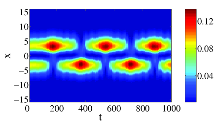
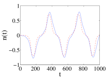
Figure 1: (Color online) Left panel: The spatiotemporal evolution of the density in the double-well potential. Right panel: the evolution of the relative difference between the numbers of atoms in the left and right wells, $n(t)$. The solid line represents the results from the integration of the GPE, while the dashed one the results obtained from the ODEs. In this case, the nonlinearity is repulsive, $g_{0}=1$, with $g_{1}=0$ and initial value $\left(|\psi|^{2}\right)_{\max}=0.1$, while parameters of the potential are $\Omega=0.1$, $V_{0}=1$ and $w=0.5$.

The next step is to vary the FRM frequency, $\omega$, at different fixed values of the FRM strength, $g_{1}$. Starting with $g_{1}=0.2$, we varied $\omega$ from $0$ to $1$ with step $1\times 10^{-4}$. The result was that, in the intervals of $0\leq\omega<0.0793$ and $\omega\geq 0.1677$, the oscillations of $n(t)$ remain periodic, like in Fig. 1, with almost the same frequency as at $g_{1}=0$, i.e. $\omega_{\mathrm{osc}}\approx 0.021$, and with the zero average value of $n(t)$, i.e., the managed system remains in the untrapped state.

However, the example displayed in Fig. 2 for $\omega=0.11$ demonstrates that the situation is completely different for

$$0.0793\leq\omega<0.1677,~{}\mathrm{i.e.,}~{}4\omega_{\mathrm{osc}}\lesssim\omega\lesssim 8\omega_{\mathrm{osc}}~{},$$ (13)

when the the system gets trapped in either of the two wells, thus exhibiting an FRM-induced SSB. Actually, for all the values of $\omega$ from interval (13), $n(t)$ does not change its sign, while the largest values of $\left|n(t)\right|$ are above $0.5$, hence the observed trapping is quite strong. In the example shown in Fig. 2, the observed frequency of the trapped oscillations is very close to half the FRM frequency: $\omega_{\mathrm{trap}}=0.054\approx\omega/2$ (note that $\omega_{\mathrm{trap}}$ is very different from the above-mentioned frequency of the oscillations in the untrapped state, $\omega_{\mathrm{osc}}\approx 0.021$). Examining the trapped states for other values of $\omega$ from interval (13), we have concluded that relation $\omega_{\mathrm{trap}}\approx\omega/2$ remains valid as long as the FRM-induced trapping holds, as seen in the left panel of Fig. 3, which displays the dependence between the values of $\omega$ and $\omega_{\mathrm{osc}}$ in the domain of $4\omega_{\mathrm{osc}}\leq\omega<8\omega_{\mathrm{osc}}$. This relation clearly suggests that the SSB trapping induced by the FRM is a result of a parametric resonance resonance . To the best of our knowledge, this is the first example of the resonant SSB in the DWP model, induced by the time-periodic drive. It is relevant to mention that the parametric resonance also plays a dominant role in effects induced by the management in the form of the time-periodic modulation of the strength of the single-well trapping potential BBB .

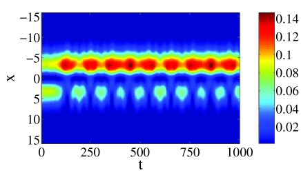
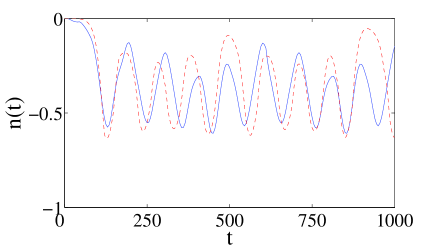
Figure 2: (Color online) The same as in Fig. 1, but in the presence of FRM with $g_{1}=0.2$, $\omega=0.11$, and initial value $\left(|\psi|^{2}\right)_{\max}=0.1$. In the right panel, the solid and dashed lines represent the results obtained from the integration of the GPE and ODEs, respectively. Other parameters are as in Fig. 1.

Next, increasing the value of the FRM amplitude to $g_{1}=0.4$, the results are as follows: for $0\leq\omega<0.0863$ and $\omega\geq 0.1581$, the condensate remains untrapped, with $n(t)$ featuring the oscillation frequency which is virtually identical to that observed in the absence of the FRM (i.e. $\omega_{\mathrm{osc}}\approx 0.021$). On the other hand, in the interval of $0.0863\leq\omega<0.1581$, which is almost identical to $4\omega_{\mathrm{osc}}\leq\omega<8\omega_{\mathrm{osc}}$, cf. its approximate counterpart in Eq. (13), the oscillations of $n(t)$ demonstrate the SSB leading to a state trapped in one potential well with maximum values of $\left|n(t)\right|$ greater than $0.5$. In this case too, we have examined the relation between the FRM frequency, $\omega$, and the frequency of the trapped oscillations, $\omega_{\mathrm{trap}}$. The obtained results corroborate that the above-mentioned parametric-resonance relation, $\omega_{\mathrm{trap}}\approx\omega/2$, remains valid, as seen in the right panel of Fig. 3.

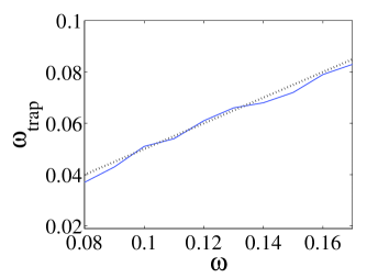
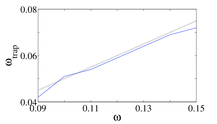
Figure 3: (Color online) The relation between the FRM  frequency, $\omega$, and frequency $\omega_{\mathrm{trap}}$ of the oscillations of the condensate spontaneously trapped in one well under the action of the FRM, in the case of the repulsive nonlinearity. Solid, and dotted lines correspond, respectively, to the result obtained from the GPE, and the estimation of $\omega_{\mathrm{trap}}=\omega/2$. Left panel: $g_{1}=0.2$ and $0.08\leq\omega<0.1677$. Right panel: $g_{1}=0.4$ and $0.09\leq\omega<0.15$. Other parameters are as in Figs. 1 and 2.

Increasing the value of $g_{1}$, we observed qualitatively the same results up to $g_{1}=0.9$, i.e., as long as the FRM amplitude, $g_{1}$, remained smaller than the average value of the repulsive-nonlinearity coefficient, $g_{0}=1$. For $g_{1}>g_{0}$, when the total nonlinearity coefficient periodically changes its sign, the situation is qualitatively different. In particular, for $g_{1}=1.2$, the SSB (trapping in one well) occurs at $0.002\leq\omega<0.011$ and $0.088\leq\omega<0.097$ [see an example in the left panels of Fig. 4, for $\omega=0.005$]. At $0.011\leq\omega<0.088$, the condensate remains untrapped [see middle panels of Fig. 4, for $\omega=0.025$], while at $\omega>0.097$ the oscillations of $n(t)$ are irregular, featuring neither symmetric oscillations nor the self-trapping [see right panels of Fig. 4, for $\omega=0.15$]. The parametric-resonance relation, $\omega_{\mathrm{trap}}\approx\omega/2$, is valid only in the interval of $0.088\leq\omega<0.097$.

Similar results were obtained for $g_{1}=1.5$. In this case, the SSB trapping occurs in the interval of $0.001\leq\omega<0.012$ [see left panels of Fig. 5, for $\omega=0.005$]. At $\omega>0.012$, $n(t)$ again features the irregular evolution, see an example in the right panels of Fig. 5, for $\omega=0.055$. Note that in these cases, corresponding to relatively large value of $g_{1}$, the Galerkin-type approximation for $n(t)$ fails to follow the result obtained in the framework of the GPE. This may be natural to expect as the large strength of the nonlinearity renders relevant the inclusion of additional modes in the description of the BEC dynamics.

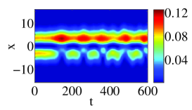
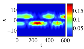
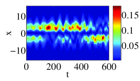
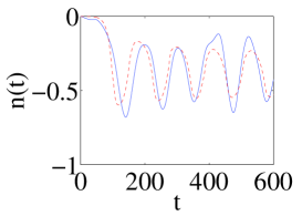
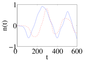
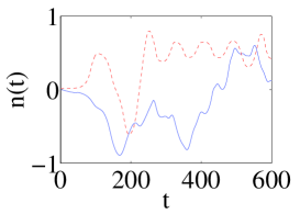
Figure 4: (Color online) The top panels show the density contour plots and the bottom panels the oscillations of the population imbalance between the two potential wells, $n(t)$, in the case of the repulsive nonlinearity with $g_{0}=1$, $g_{1}=1.2$, and initial value of $\left(|\psi|^{2}\right)_{\max}=0.1$. Left panel: $\omega=0.005$; middle panel: $\omega=0.025$; right panel: $\omega=0.15$. The parameters of the potential are the same as in the previous figures. In the bottom panels, the solid and dashed lines represent the results obtained from the integration of the GPE and ODEs, respectively.

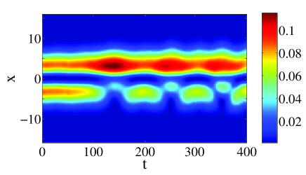
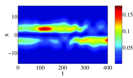
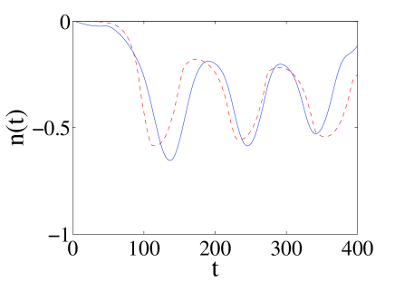
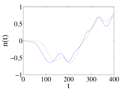
Figure 5: (Color online) The evolution of the density contour plots (top) and of $n(t)$ (bottom) in the case of the repulsive nonlinearity with $g_{0}=1$, $g_{1}=1.5$, and initial value $\left(|\psi|^{2}\right)_{\max}=0.1$. Left and right panels pertain to $\omega=0.005$ and $\omega=0.055$, respectively. The potential is the same as in the cases considered above. Additionally, In the bottom panels, the solid and dashed lines represent the results obtained from the integration of the GPE and ODEs, respectively.

III.2 “Large” initial values of the peak density

Here, we extend the analysis, increasing the initial values to $\left(|\psi|^{2}\right)_{\max}=0.17$, while all the other DWP parameters are the same as above (i.e. $\Omega=0.1$ and $V_{0}=1$). For $g_{1}=0$ (no management), the results are shown in Fig. 6. In this case, the frequency of the free oscillations of the condensate between the two wells is $\omega_{\mathrm{osc}}\approx 0.031$. The maximum value of the relative population imbalance, $n(t)$, is $0.602$, and for larger values of the initial peak density this value decreases.

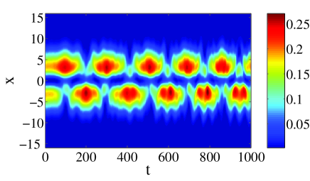
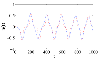
Figure 6: (Color online) The same as in Fig. 1, but for the initial value $\left(|\psi|^{2}\right)_{\max}=0.17$. In the right panel, the solid and dashed lines represent the results obtained from the integration of the GPE and ODEs, respectively. The parameters of the potential are the same as in the previous case.

Next, we study the behavior of $n(t)$ for different values of $g_{1}$ and $\omega$. For $g_{1}=0.2$, the result is that the condensate remains untrapped at $0\leq\omega<0.06341$ and $\omega>0.1009$ [similar to the situation displayed in Fig. 6], featuring the same oscillation frequency as in the absence of the management, $\omega_{\mathrm{osc}}\approx 0.031$. For $0.06341\leq\omega<0.1009$ (i.e., $2\omega_{\mathrm{osc}}\lesssim\omega\lesssim 3\omega_{\mathrm{osc}}$), the evolution of $n(t)$ suggests trapping in one well, demonstrating the SSB effect. This result is shown in Fig. 7 for $\omega=0.08$. Notice that, as observed in the right panels of Figs. 6 and 7, the agreement between the ODEs and the GPE results is fairly good.

Here, we should recall that, in the previous case, with the smaller density peaks, the observed frequency of the oscillations of the trapped BEC was following the parametric-resonance relation, $\omega_{\mathrm{trap}}=\omega/2$. As the initial density peak is getting larger, and, in particular, in the present case it corresponds to $\left(|\psi|^{2}\right)_{\max}=0.17$, this rule is no longer valid. In particular, the frequency of the trapped oscillations in the case of $\omega=0.08$ is $0.0604$.

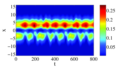
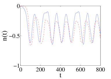
Figure 7: (Color online) The same as in Fig. 2, but for $g_{1}=0.2$, $\omega=0.08$, and initial value $\left(|\psi|^{2}\right)_{\max}=0.17$. In the right panel, the solid and dashed lines represent the results obtained from the integration of the GPE and ODEs, respectively. The other parameters are as in Fig. 2.

Next, we increase the FRM amplitude, $g_{1}$. For $g_{1}=0.4$, we have found that, at $0\leq\omega<0.0598$ and $\omega>0.0904$, the trajectory of $n(t)$ remains untrapped, with the same oscillation frequency as in the absence of the management. At $0.0598\leq\omega<0.0904$ (i.e., $2\omega_{\mathrm{osc}}\lesssim\omega\lesssim 3\omega_{\mathrm{osc}}$), the oscillations of $n(t)$ feature the self-trapping in one well.

Qualitatively the same behavior is observed for $g_{1}<0.95$. At greater values of $g_{1}$, we did not observe any self-trapping. More specifically, we examined the same two values of the FRM amplitude as above, i.e., $g_{1}=1.2$ and $g_{1}=1.5$. For $g_{1}=1.2$, we observed untrapped periodic oscillations for $0\leq\omega<0.0561$ [see the left panel of Fig. 8 for $\omega=0.01$], while for $\omega>0.02$ the population imbalance, $n(t)$, features an irregular evolution, see the right panel of Fig. 8 for $\omega=0.1$. Notice that, again, the agreement between the ODEs and GPE result is less good for this case of large nonlinearity due to the apparent involvement of higher modes in the dynamics.

Similar results were obtained for $g_{1}=1.5$. In this case, untrapped periodic oscillations occur at $0\leq\omega<0.001$, resembling the situation displayed in the left panel of Fig. 8, while, at $\omega>$ $0.001$, irregular evolution of $n(t)$ is again observed, similar to that in the right panel of Fig. 8.

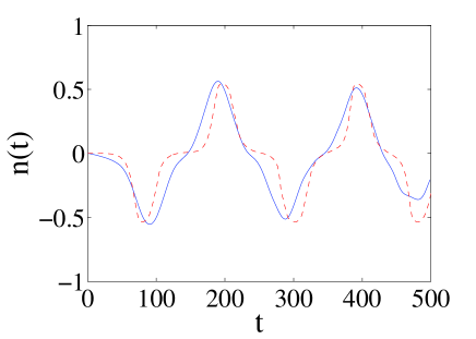
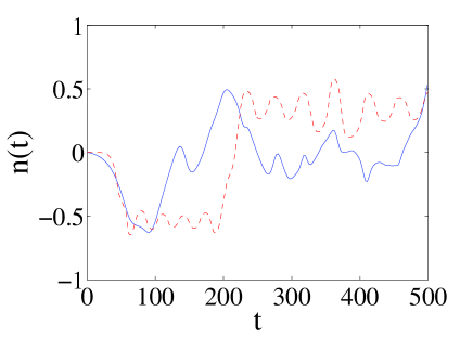
Figure 8: (Color online) Trajectories of $n(t)$ in the case of the repulsive nonlinearity with $g_{0}=1$, $g_{1}=1.2$, and initial value $\left(|\psi|^{2}\right)_{\max}=0.17$. Left and right panels pertain, respectively, to $\omega=0.01$ and $\omega=0.1$ with the same potential parameters as above. Moreover, the solid and dashed lines represent the results obtained from the integration of the GPE and ODEs, respectively.

In Table I, we summarize intervals of $g_{1}/\omega$ in which the trapped oscillations take place, in the cases of smaller and larger initial values of the peak density $(|\psi|^{2})_{max}$ [i.e., $0.1$ and $0.17$], for $g_{1}=0.2$ and $0.4$. In these cases, we observe that the trapped oscillations appear at values of $g_{1}/\omega$ similar to those presented in Ref. xie , in the framework of the two-mode approximation. However, the similarity to the two-mode approximation is lost at larger values of $g_{1}$.

Table 1: Intervals of $g_{1}/\omega$ for trapped oscillations

Initial $(|\psi|^{2})_{max}$	$g_{1}$	$g_{1}/\omega$ (interval of trapped oscillations)
$0.1$	$0.2$	$1.193\leq g_{1}/\omega\leq 2.522$
	$0.4$	$2.530\leq g_{1}/\omega\leq 4.635$
$0.17$	$0.2$	$1.982\leq g_{1}/\omega\leq 3.154$
	$0.4$	$4.424\leq g_{1}/\omega\leq 6.689$

IV The attractive nonlinearity

In the version of the DWP model with the self-attraction, we start the simulations, without the application of the FRM, for values of the parameters similar to those of Ref. theo : $g_{0}=-1$, $g_{1}=0$, $\Omega=0.1$, $V_{0}=1$, $w=0.5$, and the initial value of $\left(|\psi|^{2}\right)_{\max}=0.13$. Results of the simulations are shown in Fig. 9. In this case, the unmanaged condensate is self-trapped in one well, oscillating in it at a frequency $\omega_{\mathrm{trap,osc}}=0.046$.

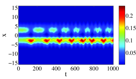
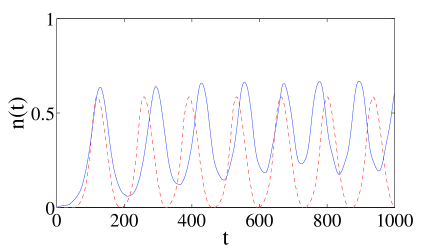
Figure 9: (Color online) The same as in Fig. 1, but in the case of the attractive nonlinearity, with $g_{0}=-1$, $g_{1}=0$, and initial value $\left(|\psi|^{2}\right)_{\max}=0.13$. In the right panel, the solid and dashed lines represent the results obtained from the integration of the GPE and ODEs, respectively. This figure and others in this section correspond to the same parameters of the potential as above, i.e., $\Omega=0.1$, $V_{0}=1$, and $w=0.5$.

In the case of the dominating attractive nonlinearity, the main effect of the FRM is opposite to that in the model with the repulsion: untrapping of the condensate which, in the unmanaged case, was trapped in the SSB state. For $g_{1}=0.2$, we have found that the untrapping occurs at

$$0.1241\leq\omega\leq 0.1594$$ (14)

(or, almost exactly, $3\omega_{\mathrm{trap,osc}}\leq\omega<4\omega_{\mathrm{trap,osc}}$). This result is shown in Fig. 10 for $\omega=0.13$. In this case, the observed frequency of the oscillations of $n(t)$ in the FRM-induced untrapped state is $\omega_{\mathrm{untrap}}=0.0318\approx\omega/4$, suggesting that this may be a manifestation of a higher-order parametric resonance resonance . Notice that, as observed in the right panels of Figs. 9 and 10, the agreement between the ODEs and the GPE results is good.

We studied the oscillations of the untrapped state for other values of $\omega$ from interval (14). It has been concluded that, at $\omega=0.12$ and $0.14$, the observed frequency of the untrapped oscillations again obeys the above-mentioned relation suggesting a higher-order parametric resonance: $\omega_{\mathrm{untrap}}=0.0298\approx\omega/4$, and $\omega_{\mathrm{untrap}}=0.0346\approx\omega/4$, respectively. In the left panel of Fig. (11), we present the relation between $\omega$ and $\omega_{\mathrm{untrap}}$ in the region of $0.124\leq\omega<0.159$. For $\omega$${<}$ $0.124$ and ${\omega>}$$0.159$, the oscillations of $n(t)$ remain trapped in a single well, with the corresponding frequency almost the same as in the absence of the management, i.e., $\omega_{\mathrm{trap,osc}}=0.046$.

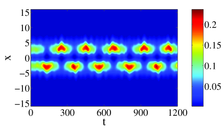
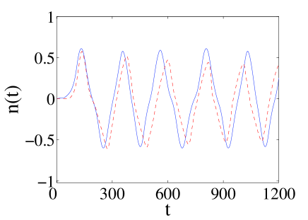
Figure 10: (Color online) The same as in Fig. 2, but in the model with the attractive nonlinearity, $g_{0}=-1$, with $g_{1}=0.2$, $\omega=0.13$, and initial value $\left(|\psi|^{2}\right)_{\max}=0.13$. In the right panel, the solid and dashed lines represent the results obtained from the integration of the GPE and ODEs, respectively.

Next, we increased the value of the FRM amplitude, $g_{1}$. For $g_{1}=0.4$, the untrapping occurred at $0.158\leq\omega<0.196$ (which almost exactly means $4\omega_{\mathrm{trap,osc}}\leq\omega<5\omega_{\mathrm{trap,osc}}$). As above, we examined the relation between $\omega$ and the respective frequency of the untrapped oscillations, $\omega_{\mathrm{untrap}}$. The results verify the same conclusion as reached above, i.e., $\omega_{\mathrm{untrap}}\approx\omega/4$. In the right panel of Fig. 11, we present the values of $\omega$ vs. $\omega_{\mathrm{untrap}}$ in the region of $0.158\leq\omega<0.196$.

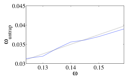
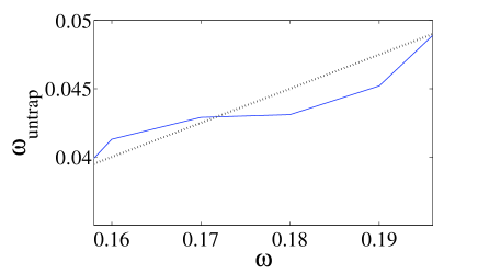
Figure 11: (Color online) The relation between $\omega$ and $\omega_{\mathrm{untrap}}$ in the model with the attractive nonlinearity. Solid, and dotted lines correspond, respectively, to the result obtained from the GPE, and the estimation of $\omega_{\mathrm{untrap}}=\omega/4$. Left panel: $g_{0}=-1$, $g_{1}=0.2$, $0.124\leq\omega<0.159$, and initial values $|\psi|^{2}=0.13$. Right panel: $g_{0}=-1$, $g_{1}=0.4$, $0.158\leq\omega<0.196$, and initial values $|\psi|^{2}=0.35$.

As in the case of the repulsive nonlinearity, we have also examined the cases with $g_{1}>|g_{0}|$, when the total nonlinearity coefficient periodically changes its sign. This was studied for $g_{1}=1.2$ and $g_{1}=1.5$. In the former case, at $0.001<\omega<0.006$ the population imbalance, $n(t)$, oscillates in the untrapped state, see the left panels of Fig. 12 for $\omega=0.003$. At $0.007\leq\omega<0.014$, we observe re-trapping after one or two untrapped oscillations, see the middle panels in Fig. 12 for $\omega=0.007$, while at $\omega>0.014$ the evolution of $n(t)$ is irregular, as seen in the right panels of Fig. 12 for $\omega=0.02$. Similar results were obtained for $g_{1}=1.5$: in this case, $n(t)$ oscillates without trapping at $0.001\leq\omega<0.004$. For $0.004\leq\omega<0.012$, we observed re-trapping after one or two oscillations, and the evolution of $n(t)$ is irregular at $\omega>0.012$. As observed in the bottom panels of Fig. 12, it is obvious that the results obtained from the ODEs and the GPE are not in agreement for values of $g_{1}>1$, for similar reasons as considered above.

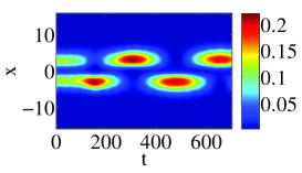
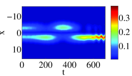
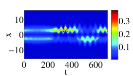
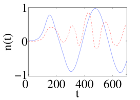
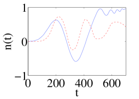
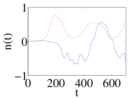
Figure 12: (Color online) Spatiotemporal contour plots (top panels) and trajectories of $n(t)$ (bottom panels) in the case of the attractive nonlinearity with $g_{0}=-1$, $g_{1}=1.2$, and initial value $\left(|\psi|^{2}\right)_{\max}=0.13$. Left panel: $\omega=0.003$; middle panel: $\omega=0.007$; right panel: $\omega=0.02$. Additionally, In the bottom panels, the solid and dashed lines represent the results obtained from the integration of the GPE and ODEs, respectively.

V Conclusions

We have studied the trapping/detrapping of Bose-Einstein condensates confined in a DWP (double-well potential), under the action of the FRM (Feshbach-resonance-management) technique. Our model is based on the Gross-Pitaevskii equation with the time-dependent nonlinear coefficient whose average value corresponds to either repulsion or attraction. We have found that the two signs give rise to different effects, regarding the trapping/detrapping of the condensate in the DWP. In the case of the self-repulsion, the BEC gets trapped in one of the two wells under the action of the FRM, if it was untrapped in the unmanaged state. We have found the range of values of the driving frequency leading to this effect. If the sign of the nonlinearity does not change due to the time-periodic modulation, and the densities are sufficiently low, as mentioned above, the frequency of the intrinsic oscillations of the FRM-induced trapped states is half the management frequency, which suggests a parametric resonance as an underlying mechanism.

On the other hand, in the case of the self-attractive nonlinearity (on the average), we observe the opposite phenomenon: the application of the FRM results in untrapped oscillations, if the unmanaged condensate was self-trapped in one of the two wells. If the periodically modulated nonlinearity does not change its sign, the frequency of the untrapped oscillations supported by the FRM is almost exactly equal to a quarter of the driving frequency, suggesting a higher-order parametric resonance as an underlying mechanism. It is worth mentioning here that, this frequency relation, is relevant, as in the previous case, for sufficiently low densities.

Our results were corroborated with ones derived in the framework of a semi-analytical approach. The latter, was based on an a Galerkin-type expansion that was used to describe the evolution of the wavefunctions at each well of the DWP. This led to a non-autonomous system of ODEs, which were solved numerically to find the relative difference in the atomic population between the two wells. In all cases, the ODE result was compared to the one obtained by the GPE model, and they were found to be in fairly good agreement: in particular, we found a quantitatively good agreement for small values of the modulation depth, $g_{1}<1$ (in both repulsive and attractive cases), and a qualitatively good agreement for $g_{1}>1$ (for the repulsive case). Our approximation was found to fail only for $g_{1}>1$ in which case the strong nonlinearity causes the involvement of additional modes in the dynamics.

Detailed analysis of the resonances that may explain the character of the FRM-induced trapping and detrapping is a nontrivial problem, because the two-mode approximation, such as the one presented above or the one recently proposed in Ref. xie , is insufficient for this purpose. The development of a more sophisticated finite-mode approximation, that may help uncover the resonances, is a subject for a separate study. Another challenging possibility is to consider similar dynamical effects in multidimensional settings. It may also be interesting to extend the analysis to the case of a binary BEC mixture trapped in a DWP. These problems will also be considered elsewhere.

Acknowledgments. B.A.M. appreciates a support from the German-Israel Foundation through grant No. 149/2006. P.G.K. gratefully acknowledges the support of NSF-DMS-0349023 (CAREER), NSF-DMS-0806762 and of the Alexander von Humboldt Foundation. The work of D.J.F. was partially supported by the Special Account for Research Grants of the University of Athens.

References

- (1) C. J. Pethick and H. Smith, Bose-Einstein condensation in dilute gases, Cambridge University Press (Cambridge, 2002).
- (2) L. P. Pitaevskii and S. Stringari, Bose-Einstein Condensation, Oxford University Press (Oxford, 2003).
- (3) P. G. Kevrekidis, D. J. Frantzeskakis, and R. Carretero-González (eds.), Emergent nonlinear phenomena in Bose-Einstein condensates. Theory and experiment (Springer-Verlag, Berlin, 2008).
- (4) R. Carretero-González, D. J. Frantzeskakis, and P. G. Kevrekidis, Nonlinearity 21, R139 (2008).
- (5) A. E. Leanhardt, Y. Shin, D. Kielpinski, D. E. Pritchard, and W. Ketterle, Phys. Rev. Lett. 90, 140403 (2003); W. Zhang, Ö. E. Müstecaplioglu, and L. You, Phys. Rev. A 75, 043601 (2007); H. E. Nistazakis, D. J. Frantzeskakis, P. G. Kevrekidis, B. A. Malomed, R. Carretero-González, and A. R. Bishop, Phys. Rev. A 76, 063603 (2007).
- (6) K. E. Strecker, G. B. Partridge, A. G. Truscott, and R. G. Hulet, Nature 417, 150 (2002).
- (7) L. Khaykovich, F. Schreck, G. Ferrari, T. Bourdel, J. Cubizolles, L. D. Carr, Y. Castin, and C. Salomon, Science 296, 1290 (2002).
- (8) S. L. Cornish, S. T. Thompson, and C. E. Wieman, Phys. Rev. Lett. 96, 170401 (2006).
- (9) S. Burger, K. Bongs, S. Dettmer, W. Ertmer, K. Sengstock, A. Sanpera, G. V. Shlyapnikov, and M. Lewenstein, Phys. Rev. Lett. 83, 5198 (1999).
- (10) J. Denschlag, J. E. Simsarian, D. L. Feder, C. W. Clark, L. A. Collins, J. Cubizolles, L. Deng, E. W. Hagley, K. Helmerson, W. P. Reinhardt, S. L. Rolston, B. I. Schneider, and W. D. Phillips, Science 287, 97 (2000).
- (11) B. P. Anderson, P. C. Haljan, C. A. Regal, D. L. Feder, L. A. Collins, C. W. Clark, and E. A. Cornell, Phys. Rev. Lett. 86, 2926 (2001).
- (12) Z. Dutton, M. Budde, Ch. Slowe, and L. V. Hau, Science 293, 663 (2001).
- (13) C. Becker, S. Stellmer, P. Soltan-Panahi, S. Dörscher, M. Baumert, E.-M. Richter, J. Kronjäger, K. Bongs, and K. Sengstock, Nature Phys. 4, 496 (2008).
- (14) S. Stellmer, C. Becker, P. Soltan-Panahi, E.-M. Richter, S. Dörscher, M. Baumert, J. Kronjäger, K. Bongs, and K. Sengstock, Phys. Rev. Lett. 101, 120406 (2008).
- (15) A. Weller, J. P. Ronzheimer, C. Gross, D. J. Frantzeskakis, G. Theocharis, P. G. Kevrekidis, J. Esteve, and M. K. Oberthaler, Phys. Rev. Lett. 101, 130401 (2008).
- (16) I. Shomroni, E. Lahoud, S. Levy, and J. Steinhauer, Nature Phys. 5, 193 (2008).
- (17) G. Theocharis, A. Weller, J. P. Ronzheimer, C. Gross, M. K. Oberthaler, P. G. Kevrekidis, and D. J. Frantzeskakis, arXiv:0909.2122.
- (18) B. Eiermann, Th. Anker, M. Albiez, M. Taglieber, P. Treutlein, K.-P. Marzlin, and M. K. Oberthaler, Phys. Rev. Lett. 92, 230401 (2004).
- (19) Yu. S. Kivshar and G. P. Agrawal, Optical Solitons: From Fibers to Photonic Crystals, Academic Press (San Diego, 2003).
- (20) M. Albiez, R. Gati, J. Fölling, S. Hunsmann, M. Cristiani, and M. K. Oberthaler, Phys. Rev. Lett. 95, 010402 (2005).
- (21) T. Zibold, E. Nicklas, C. Gross, and M.K. Oberthaler Phys. Rev. Lett. 105, 204101 (2010)
- (22) S. Raghavan, A. Smerzi, S. Fantoni, and S. R. Shenoy, Phys. Rev. A 59, 620 (1999); S. Raghavan, A. Smerzi and V. M. Kenkre, Phys. Rev. A 60, R1787 (1999); A. Smerzi and S. Raghavan, Phys. Rev. A 61, 063601 (2000).
- (23) E. A. Ostrovskaya, Y. S. Kivshar, M. Lisak, B. Hall, F. Cattani, and D. Anderson, Phys. Rev. A 61, 031601 (R) (2000).
- (24) K. W. Mahmud, J. N. Kutz and W. P. Reinhardt, Phys. Rev. A 66, 063607 (2002).
- (25) V. S. Shchesnovich, B.A. Malomed, and R. A. Kraenkel, Physica D 188, 213 (2004).
- (26) D. Ananikian, and T. Bergeman, Phys. Rev. A 73, 013604 (2006).
- (27) P. Ziń, E. Infeld, M. Matuszewski, G. Rowlands, and M. Trippenbach, Phys. Rev. A 73, 022105 (2006).
- (28) T. Kapitula and P. G. Kevrekidis, Nonlinearity 18, 2491 (2005).
- (29) G. Theocharis, P. G. Kevrekidis, D. J. Frantzeskakis and P. Schmelcher, Phys. Rev. E 74, 056608 (2006).
- (30) D. R. Dounas-Frazer, A. M. Hermundstad, and L .D. Carr, Phys. Rev. Lett. 99, 200402 (2007).
- (31) C. Cambournac, T. Sylvestre, H. Maillotte, B. Vanderlinden, P. Kockaert, Ph. Emplit, and M. Haelterman, Phys. Rev. Lett. 89, 083901 (2002).
- (32) P. G. Kevrekidis, Z. Chen, B. A. Malomed, D. J. Frantzeskakis, and M. I. Weinstein, Phys. Lett. A 340, 275 (2005).
- (33) M. Ornigotti, G. Della Valle, D. Gatti, and S. Longhi, Phys. Rev. A 76, 023833 (2007).
- (34) N. Tsukada, M. Gotoda, Y. Nomura, and T. Isu, Phys. Rev. A 59, 3862 (1999); M. Holthaus and S. Stenholm, Eur. Phys. J. B 20, 451 (2001); R. Khomeriki, S. Ruffo, and S. Wimberger, EPL 77, 40005 (2007); Q. Xie and W Hai, Phys. Rev. A 80, 053603 (2009).
- (35) T. Köhler, K. Goral and P. S. Julienne, Rev. Mod. Phys.78, 1311 (2006).
- (36) S. Inouye, M. R. Andrews, J. Stenger, H. J. Miesner, D. M. Stamper-Kurn and W. Ketterle, Nature 392, 151 (1998); J. Stenger, S. Inouye, M. R. Andrews, H.-J. Miesner, D. M. Stamper-Kurn, and W. Ketterle, Phys. Rev. Lett. 82, 2422 (1999); J. L. Roberts, N. R. Claussen, J. P. Burke Jr., C. H. Greene, E. A. Cornell, and C. E. Wieman, Phys. Rev. Lett. 81, 5109 (1998); S. L. Cornish, N. R. Claussen, J. L. Roberts, E. A. Cornell, and C. E. Wieman, Phys. Rev. Lett. 85, 1795 (2000).
- (37) F. K. Fatemi, K. M. Jones, and P. D. Lett, Phys. Rev. Lett. 85, 4462 (2000); M. Theis, G. Thalhammer, K. Winkler, M. Hellwig, G. Ruff, R. Grimm, and J. H. Denschlag, Phys. Rev. Lett. 93, 123001 (2004).
- (38) I. Towers and B. A. Malomed, J. Opt. Soc. Am. 19, 537 (2002); see also for an experimental realization (although with a different ) M. Centurion, M.A. Porter, P. G. Kevrekidis and D. Psaltis, Phys. Rev. Lett. 97, 033903 (2006), M. Centurion, M.A. Porter, Y. Pu, P. G. Kevrekidis, D. J. Frantzeskakis and D. Psaltis, Phys. Rev. Lett. 97, 234101 and Phys. Rev. A 75, 042902 (2008).
- (39) F. Kh. Abdullaev, J. G. Caputo, R. A. Kraenkel, and B. A. Malomed, Phys. Rev. A 67, 013605 (2003); H. Saito and M. Ueda, Phys. Rev. Lett. 90, 040403 (2003); G. D. Montesinos, V. M. Pérez-García, and P. J. Torres, Physica D 191 193 (2004).
- (40) P. G. Kevrekidis, G. Theocharis, D. J. Frantzeskakis, and B. A. Malomed, Phys. Rev. Lett. 90, 230401 (2003); D. E. Pelinovsky, P. G. Kevrekidis, and D. J. Frantzeskakis, Phys. Rev. Lett. 91, 240201 (2003); D. E. Pelinovsky, P. G. Kevrekidis, D. J. Frantzeskakis, and V. Zharnitsky, Phys. Rev. E 70, 047604 (2004); Z. X. Liang, Z. D. Zhang, and W. M. Liu, Phys. Rev. Lett. 94, 050402 (2005); M. Matuszewski, E. Infeld, B. A. Malomed, and M. Trippenbach, Phys. Rev. Lett. 95, 050403 (2005).
- (41) G. Theocharis, P. Schmelcher, P. G. Kevrekidis and D. J. Frantzeskakis, Phys. Rev. A 72, 033614 (2005).
- (42) F. Kh. Abdullaev and M. Salerno, J. Phys. B 36, 2851 (2003).
- (43) M. I. Rodas-Verde, H. Michinel, and V. M. Pérez-García, Phys. Rev. Lett. 95, 153903 (2005); A. V. Carpenter, H. Michinel, M. I. Rodas-Verde, and V. M. Pérez-García, Phys. Rev. A 74, 013619 (2006).
- (44) H. Sakaguchi and B. A. Malomed, Phys. Rev. E 72, 046610 (2005); Phys. Rev. A 81, 013624 (2010).
- (45) G. Theocharis, P. Schmelcher, P. G. Kevrekidis and D. J. Frantzeskakis, Phys. Rev. A 74, 053614 (2006).
- (46) F. Kh. Abdullaev, and J. Garnier, Phys. Rev. A 74, 013604 (2006).
- (47) G. Dong, B. Hu, and W. Lu, Phys. Rev. A 74, 063601 (2006).
- (48) Yu. V. Bludov, V. A. Brazhhyi, and V. V. Konotop, Phys. Rev. A 76, 023603 (2007).
- (49) T. Mayteevarunyoo, B. A. Malomed, and G. Dong, Phys. Rev. A 78, 053601 (2008).
- (50) H. Sakaguchi and B. A. Malomed, Phys. Rev. A 81, 013624 (2010).
- (51) Q. Xie, Phys. Lett. A 373,173 (2009).
- (52) G. Theocharis, P.G. Kevrekidis, H.E. Nistazakis, D.J. Frantzeskakis , A.R. Bishop, Phys. Lett. A 337, 441-448 (2005).
- (53) L. D. Landau and E. M. Lifshitz, Mechanics (Nauka Publishers: Moscow, 1988).
- (54) B. B. Baizakov, G. Filatrella, B. A. Malomed, and M. Salerno, Phys. Rev. E 71, 036619 (2005).