Detection of Flux Emergence, Splitting, Merging, and Cancellation in the Quiet Sun

Abstract

We investigate the frequency of magnetic activities, namely flux emergence, splitting, merging, and cancellation, through an automatic detection in order to understand the generation of the power-law distribution of magnetic flux reported by Parnell et al. (2009). Quiet Sun magnetograms observed in the Na i 5896 Å line by the Hinode Solar Optical Telescope is used in this study. The longitudinal fluxes of the investigated patches range from $\approx 10^{17}$ Mx to $\approx 10^{19}$ Mx. Emergence and cancellation are much less frequent than merging and splitting. The time scale for splitting is found to be $\approx 33$ minutes and independent of the flux contained in the splitting patch. Moreover magnetic patches split into any flux contents with an equal probability. It is shown that such a fragmentation process leads to a distribution with a power-law index $-2$. Merging has a very weak dependence on flux content, with a power-law index of only $-0.33$. These results suggest that (1) magnetic patches are fragmented by splitting, merging, and tiny cancellation; and (2) flux is removed from the photosphere through tiny cancellations after these fragmentations.

¹University of Tokyo, Japan

²Lockheed Martin Space and Astrophysical Laboratory, USA

1 Introduction

The surface magnetic activities are the source of various phenomena and one of the most important targets for solar studies. Parnell et al. (2009) found that the magnetic flux content of the solar surface has a power-law distribution spanning the range from large active regions to small patches in the quiet network that are concentrated near supergranular boundaries. This suggests that they are generated by the same mechanism, or that they are dominated by the same magnetic processes: emergence, splitting, merging, and cancellation. The relationship between the flux distribution and these activities is described by the magneto-chemistry (MC) equation (Schrijver et al. 1997). Although some special cases of the MC equation reproduce the power-law spectra of magnetic flux content (Parnell 2002), there remain open questions. Observational studies of the frequencies of the four magnetic activities mentioned above give important clues to this problem. Here we investigate magnetograms to quantify the flux dependence of these magnetic activities by means of an automatic detection. We concentrate on the quiet Sun because the activities there are more moderate than in active regions.

2 Observation

We use magnetograms in Na i D 5896 Å obtained by the Narrow-band Filter Imager (NFI) of the Solar Optical Telescope (SOT) onboard the Hinode satellite. The observation period is 00:30 UT – 04:09 UT on November 11, 2009. The time cadence is 1 minute. The field of view is $112\hbox{${}^{\prime\prime}$}\times 112\hbox{${}^{\prime\prime}$}$. Hinode observed near the disk center during this period. The upper panel of Fig. 1 shows an example of the magnetograms. It is possible that not all internetwork patches are observed even at the Hinode resolution (see the flattened flux distribution in Parnell et al. 2009). We focus on network patches to avoid this observational limit. Dark current and flat field of CCD camera are removed by using the procedure fg_prep.pro included in the SolarSoft package. The average of each line is subtracted to remove a tip side effect of the CCD camera (Lamb et al. 2010). We rotate all the magnetograms to the position at 02:03 UT by taking account of the solar differential rotation. The images were aligned to remove residual spacecraft jitter. The Stokes V/I signal is converted to magnetic field strength after these processes. The conversion coefficient is taken to be 8645 G/DN from a comparison between a Stokes V/I image and an MDI magnetogram which were acquired within one minute. We smear the magnetic field data with a scale of three pixels in space and average it over five images in time.

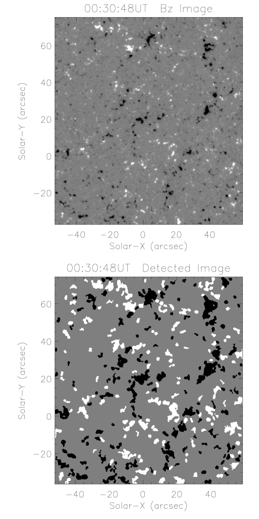
Figure 1.: Top: Na i D magnetogram obtained by Hinode/SOT at 00:30 UT on November 11, 2009. Bottom: Two-valued magnetogram for detected patches corresponding to the upper panel.

3 Detection of Magnetic Activities

Our procedure to investigate magnetic activities consists of (1) detection and tracking of magnetic patches, (2) detection of splittings and mergings, and (3) detection of emergences and cancellations.

We detect magnetic patches by means of a clumping method, in which a patch is defined as a massif of pixels having signals above a threshold (Parnell et al. 2009). The threshold for magnetic field is set as $2\sigma$. The value of $2\sigma$ is obtained from a Gaussian fit to the magnetic field strength distribution and turns out to be about 10 G. We also set a size threshold of 81 pixels for the massifs, which corresponds to the typical size of granules. The lower panel of Fig. 1 shows a two-valued magnetogram computed with these thresholds. We can see that the detected features are mainly network patches and that most internetwork patches are removed. Tracking is done by checking the spatial overlap of patches in consecutive images (Hagenaar 1999). However, there are many overlaps of multiple patches at the Hinode resolution. Thus we set two additional conditions for tracking: (A) tracking is done from the patches with larger flux content, and (B) if there are more than two overlapping patches, the one having the closest flux content is selected. These conditions are based on the concept that smaller flux patches tend to go below the detection threshold (condition A) and that the flux change between consecutive images is moderate (condition B).

Detection of splittings and mergings is also done by checking the overlap between consecutive images. More specifically, the conditions for splitting are the following: (C) more than two patches overlap a patch from the previous image; and (D) more than one overlapping patch is newly produced, i.e., it did not exist in the previous image. Conditions C and D guarantee that one or more new patches overlap the previous one. Merging is defined as the same process in time-reversed magnetograms.

Emergences/cancellations are detected as a pair of flux increase/decrease events in different polarities after removing those due to splittings and mergings. We define a flux change event as (E) a flux increase or decrease for more than 5 minutes with ${\rm d}\phi/{\rm d}t>3.5\times 10^{18}$ Mx. The threshold for $d\phi/dt$ is taken to be the typical flux change rate of cancellations because a cancellation is thought to be a more moderate event in flux change than an emergence (Chae et al. 2001).

4 Results

Table 1.: Number of magnetic patches and magnetic activities

	Positive	Negative
Number of patches	1636	1637
Splitting	493	482
Merging	536	535
Emergence	3
Cancellation	86

Table 1 shows the total number of detected magnetic patches and magnetic activities. There are enough splittings and mergings for a statistical investigation but not enough emergences and cancellations. Because splitting and merging of more than three patches occur in less than 5% of the cases, they will be ignored in what follows.

Figure 2a shows the flux distribution of the detected magnetic patches. The dotted/broken lines indicate the distribution of positive/negative patches, respectively, and the solid line indicates the distribution of all the magnetic patches. The dashed line represents a linear fit to the flux distribution of all patches between $10^{17.5}$ Mx and $10^{19}$ Mx. The fit indicates $\phi^{-1.78}$, where $\phi$ is the flux content of each patch and the error of the fitted index is $\approx 0.05$. Within the accuracy of our results, this dependence is almost the same as the one obtained by Parnell et al. (2009), $\phi^{-1.85}$. The distribution drops down below $\phi_{\rm{th}}=10^{17.5}$ Mx, which we define as a detection limit in this study. We cannot detect all the patches below the limit, so from now on we only investigate patches with fluxes larger than $\phi_{\rm{th}}$.

The solid line in Fig. 2b shows the flux distribution of splitting patches divided by patch density, which means the average splitting probability density for each patch. We can see that the distribution is almost flat much above the detection limit, implying that the probability density of splitting is independent of flux content. The probability density of observed splittings $K(\phi)$ can be expressed as

$$K(\phi)=\int_{0}^{\phi}k(x,\phi-x)\ {\rm d}x=\rm{constant}\;\;(\rm{for\ all}\ \phi),$$ (1)

where $k(x,y)$ is the splitting probability density distribution into flux content $x$ and $y$. Around the detection limit, the probability density is falling down. This falling down is explained by splitting into fluxes below the detection limit. We need another condition of splitting besides Equation 1—how the flux content is split—to estimate the dropping around the detection limit. We assume that patches split into elements of any flux content with equal probability, namely

$$k(x,\phi-x)=\rm{constant}\ (\rm{for}\ \it{x}).$$ (2)

Figure 2.: (a): Distribution of magnetic flux contained in magnetic patches. The solid/dotted/broken lines indicate the observed flux distribution of all/positive/negative patches, respectively. The dashed line represents a linear fit between $10^{17.5}$ Mx and $10^{19}$ Mx. The slope of the fitted line is $-1.78$, showing nearly the same power law distribution reported by Parnell et al. (2009). The vertical line indicates the lower limit for the validity of the power law distribution in this study, which corresponds to the detection limit ($=10^{17.5}$ Mx). (b): Observed probability density distribution of splitting flux patches (solid) and an analytical probability density distribution for random splitting with a timescale of $33$ minutes (dashed). The horizontal and vertical lines indicate the probability densities corresponding to $33$ minutes and the detection limit. (c): Observed probability density distribution of merging flux patches (solid) and linear fit (dashed). The slope of the fitted line is $0.33$. The vertical line marks the detection limit.

Equations 1 and 2 lead to the following analytic form for the probability density distribution of flux content for splitting patches

$$k(x,y)=\frac{K_{0}}{x+y},$$ (3)

where $K_{0}$ represents the typical time constant for splittings. Now we can estimate the falling down effect of splitting into flux below the detection limit as

$$K(\phi;\phi_{\rm{th}})=\int_{\phi_{\rm{th}}}^{\phi-\phi_{\rm{th}}}k(x,\phi-x)\,{\rm d}x=K_{0}\,(1-\frac{\phi_{\rm{th}}}{\phi}).$$ (4)

The dashed curve in Fig. 2b indicates $K(\phi;\phi_{\rm{th}})$ with $K_{0}=1.0\times 10^{-3}$ $\rm{s}^{-1}$. This estimated line fits the falling down of the observed distribution well, which supports the assumption that patches split into any flux content with equal probability.

Figure 2c shows the flux distribution of merging flux. The solid line represents the observed distribution normalized by patch density, which indicates the probability of merging of one patch. There are no effect of $\phi_{\rm{th}}$ because the flux content after merging is larger than before the merging. The dashed line indicates a fit of the form $\phi^{-0.33}$.

5 Discussion

5.1 Power-law Distribution Generated by Splitting Process

By using the obtained dependence of splitting on flux content, we derive the flux distribution achieved through the accumulation of this process. The MC equation for splitting can be written as

$$\frac{\partial n(\phi)}{\partial t}=2\int_{\phi}^{\infty}n(x)k(\phi,x-\phi)\,{\rm d}x-\int_{0}^{\phi}n(\phi)k(x,\phi-x)\,{\rm d}x$$ (5)

where $n(\phi)$ represents the flux distribution. After substituting $k(x,y)=K_{0}/(x+y)$ and differentiating with respect to $\phi$, we obtain

$$\frac{\partial^{2}n(\phi)}{\partial\phi\partial t}=-\frac{K_{0}}{\phi^{2}}\frac{\partial}{\partial\phi}\left[\phi^{2}n(\phi)\right].$$ (6)

This equation has a time-independent solution $n(\phi)\propto\phi^{-2}$.

5.2 Importance of Tiny Cancellations

We note here that cancellation may play an important role in the generation of the observed power-law flux distribution. Figure 3 shows a schematic view of our model. For the flux distribution we consider a power law of index $-\gamma$ which, according to the observations, is in the range $1.5<\gamma<2$. The total flux amount can be calculated as

$$\Phi_{\rm tot}=\int_{\phi_{\rm min}}^{\phi_{\rm max}}\phi\,n(\phi)\,{\rm d}\phi\propto\phi_{\rm max}^{-\gamma+2},$$ (7)

where the rightmost side is valid for $\gamma<2$. This shows that the total flux is dominated by $\phi_{\rm max}$. We obtain the total flux loss by cancellations as

$$\left.\frac{\partial\Phi_{\rm tot}}{\partial t}\right|_{\rm canc}=\int_{\phi_{\rm{min}}}^{\phi_{\rm{max}}}\phi\frac{\partial n_{\rm{canc}}(\phi)}{\partial t}\,{\rm d}\phi\propto\phi_{\rm{min}}^{-2\gamma+3}.$$ (8)

This implies that tiny cancellations play an important role in flux balance.

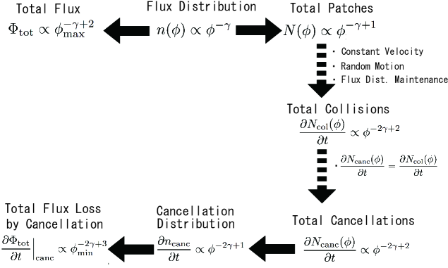
Figure 3.: A model for the flux distribution of magnetic patches and cancellations with $1.5<\gamma<2$. Solid arrows indicate mathematical relations, while dashed arrows indicate relationships with some physical assumptions. Note that the total flux is dominated by $\phi_{\rm{max}}$ but that the total flux loss is dominated by $\phi_{\rm{min}}$ in this model.

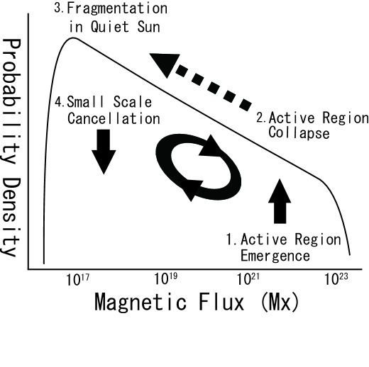
Figure 4.: A schematic picture of the flux transport mechanism. The total flux is dominated by large emerged fluxes. Emerged fluxes are fragmented through splittings, mergings, and cancellations with tiny magnetic patches. Cancellations become dominant in tiny patches (see Fig. 3 and related discussion).

5.3 Global Flux Transport Speculation

In Figure 4 we speculate on the flux transport on a global scale. The magnetic flux from active regions is mainly fragmented by pure splittings and cancellations with tiny patches. They will submerge through cancellations when they are fragmented enough. These speculations should be confirmed in the future with a full understanding of the four magnetic activities discussed in the present paper.

Acknowledgments

We thank all the members of the Hinode team and the GCOE program ‘From the Earth to Earths’, which supported a stay in Lockheed Martin Space and Astronomical Laboratory. We also thank the members of Lockheed Martin Space and Astronomical Laboratory for plentiful discussions.

References

- Chae et al. (2001) Chae, J., Wang, H., Qiu, J., Goode, P. R., Strous, L., & Yun, H. S. 2001, ApJ, 560, 476
- Hagenaar (1999) Hagenaar, H. J. 1999, Ph.D. thesis, Universiteit Utrecht
- Lamb et al. (2010) Lamb, D. A., DeForest, C. E., Hagenaar, H. J., Parnell, C. E., & Welsch, B. T. 2010, ApJ, 720, 1405
- Parnell (2002) Parnell, C. E. 2002, MNRAS, 335, 389
- Parnell et al. (2009) Parnell, C. E., DeForest, C. E., Hagenaar, H. J., Johnston, B. A., Lamb, D. A., & Welsch, B. T. 2009, MNRAS, 698, 75
- Schrijver et al. (1997) Schrijver, C. J., Title, A. M., van Ballegooijen, A. A., Hagenaar, H. J., & Shine, R. A. 1997, ApJ, 487, 424