Cramér-Rao Bound for Blind Channel Estimators in Redundant Block Transmission Systems

Abstract

In this paper, we derive the Cramér-Rao bound (CRB) for blind channel estimation in redundant block transmission systems, a lower bound for the mean squared error of any blind channel estimators. The derived CRB is valid for any full-rank linear redundant precoder, including both zero-padded (ZP) and cyclic-prefixed (CP) precoders. A simple form of CRBs for multiple complex parameters is also derived and presented which facilitates the CRB derivation of the problem of interest. A comparison is made between the derived CRBs and performances of existing subspace-based blind channel estimators for both CP and ZP systems. Numerical results show that there is still some room for performance improvement of blind channel estimators.

I Introduction

Block transmission systems, especially orthogonal frequency-division multiplexing (OFDM) systems, have become one of the most popular solutions to meet the high data rate requirements of modern communication standards. For example, wireless local-area networks (WLAN) standards such as IEEE 802.11n [5], and beyond third-generation (B3G) cellular communication standards such as IEEE 802.16e [6] or 3GPP-LTE [7], all apply block transmission schemes as the basic physical-layer transmission scheme. Channel estimation is crucial for equalization in these systems. Most of the modern standards using block transmission systems insert some already-known symbols, called pilot symbols, in the transmitted signals, and the receiver estimates the channel response from the pilot symbols [8]. Such an approach is called pilot-assisted channel estimation method. However, pilot assisted methods suffer from loss of bandwidth efficiency since the inserted pilot symbols do not carry any information.

Blind channel estimation in block transmission systems, on the other hand, aims to avoid the redundancy introduced by pilot symbols. The goal of blind channel estimation is to estimate the channel response directly from unknown symbols, which can be data symbols . Current blind channel estimation algorithms can be roughly divided into two main categories. The first exploits the fact that all of the transmitted symbols come from a set of finite number of points in the signal space, i.e., the modulation constellation [10]. The second assumes no a priori information about the modulation constellation at the receiver side and consists mostly of subspace-based methods [11]. This kind of approach can be applied in a wider range of situations, but may have a slightly worse performance than finite-alphabet methods. This paper addresses only the performance bound of blind channel estimators assuming no a priori information about the transmitted signals.

Cramér-Rao bound (CRB) is an important performance bound which gives a lower bound for the mean squared error (MSE) of channel estimators in a communication system [8]. A CRB for blind finite impulse response (FIR) multichannel estimation has been derived in [12]. It is, however, not applicable for redundant block transmission systems. There are two main types of redundant block transmission systems, namely, systems with null guard intervals, also known as zero padded (ZP) systems, and systems with cyclic prefixes (CP). The CRB for blind channel estimators in ZP block transmission systems has been derived in [1, 2]. But the CRB for blind channel estimators in CP block transmission systems, to our best knowledge, has not yet been studied in the literature. In this paper, a general CRB for block transmission systems is derived, which is valid for any linear redundant precoders, including those in ZP [13] and CP systems. We then compare the performances of existing blind channel estimators [3, 4, 9, 14] with the derived CRB.

An additional contribution of this paper is a simplification of CRB formulas for complex parameters. To calculate the CRB for blind channel estimation in wireless communication systems, in which numerical values are usually modeled by complex numbers, we extend the existing results of CRBs for unconstrained and constrained parameters, originally for real parameters [17, 15, 16], to the case of multiple complex parameters. We devote one section to do this work before starting the derivation of the CRB for the problem of interest.

There has been some existing literature on this topic [18, 19, 20, 21]. In [18, 19, 21], the derived CRBs for unconstrained and constrained complex parameters, unlike the corresponding CRBs for real parameters, are variance bounds of any unbiased estimators for $[\begin{array}[]{cc}\bm{\theta}^{T}&\bm{\theta}^{H}\end{array}]^{T}\in\mathbb{C}^{2n}$, a vector of double size of the unknown parameter vector $\bm{\theta}\in\mathbb{C}^{n}$. In [20], a CRB that represents variance bound of unbiased estimators for $\bm{\theta}\in\mathbb{C}^{n}$ is presented for the first time. However, its result is in a complicated form compared with the well known CRB for real parameters [16]. In addition, the result in [20] does not consider constraints on unknown parameters and cannot be directly applied in the problem considered in this paper.

Instead of a complicated form, we seek here to derive simple CRBs for unconstrained and constrained complex parameters in a form similar to those for real parameters. Specifically, the form of the derived CRB for unconstrained complex parameters is exactly identical to the CRB for unconstrained real parameters; and if the constraint function is holomorphic, the CRB for constrained complex parameters can also have the same form as that of the CRB for constrained real parameters [16]. Using this result, the derivation of CRB for the blind channel estimation problem becomes simple and compact compared to that in [1].

The rest of the paper is organized as follows. In Section II, we derive simple CRBs for unconstrained and constrained complex parameters. In Section III, the system model of a redundant block transmission system is described and the blind channel estimation problem is formulated. We then derive the CRB for blind channel estimators in Section IV, using results given in Section II. In Section V, numerical results are conducted to compare the derived CRB with performances of existing blind channel estimators. Conclusions and future work are presented in Section VI.

Notations

Bold-faced lower case letters represent column vectors, and bold-faced upper case letters are matrices. Superscripts such as in $\bm{v}^{*}$, $\bm{v}^{T}$, $\bm{v}^{H}$, $\bm{M}^{-1}$, and $\bm{M}^{\dagger}$ denote the conjugate, transpose, conjugate transpose (Hermitian), inverse, and Moore-Penrose generalized inverse of the corresponding vector or matrix. The vector $\mathsf{vec}(\bm{M})$ denotes the column vector formed by stacking all columns of $\bm{M}$. The vector $\mathsf{E}\left[\bm{v}\right]$ denotes the expectation of $\bm{v}$, and the matrix $\mathsf{E}\left[\bm{M}\right]$ denotes the expectation of $\bm{M}$. The matrix $\mathsf{cov}(\bm{u},\bm{v})$ denotes the cross-covariance matrix of random vectors $\bm{u}$ and $\bm{v}$ and is defined as $\mathsf{cov}(\bm{u},\bm{v})\triangleq\mathsf{E}\left[(\bm{u}-\mathsf{E}(\bm{u}))(\bm{v}-\mathsf{E}(\bm{v}))^{H}\right]$. The Kronecker product of $\bm{A}$ and $\bm{B}$ is denoted by $\bm{A}\otimes\bm{B}$. The notation $\bm{A}\geq\bm{B}$ means that $\bm{A}-\bm{B}$ is a nonnegative-definite matrix. The trace of a square matrix $\bm{A}$ is denoted by $\mathsf{tr}(\bm{A})$. Matrices $\bm{I}_{n}$ and $\bm{0}_{m\times n}$ denote the $n\times n$ identity matrix and the $m\times n$ zero matrix, respectively. Notations $[\bm{A}]_{i,j}$ and $[\bm{v}]_{i}$ refer to the $(i,j)$th entry of matrix $\bm{A}$ and the $i$th element of vector $\bm{v}$, respectively. The notation $[\bm{v}]_{a:b}$ denotes the column vector whose elements contain the $a$th through $b$th elements of vector $\bm{v}$.

II Simple Forms of CRBs for Complex Parameters

In this section, we present an extension of CRBs originally for unconstrained and constrained real parameters to the case of complex parameters. The CRB for constrained complex parameters derived in this section, in particular, will be directly used in Section IV for CRB derivation for blind channel estimators in redundant block transmission systems.

II-A CRB for Unconstrained Complex Parameters

Suppose that $\bm{\theta}\in\mathbb{C}^{n}$ is an unknown complex parameter vector, and $\bm{t}(\bm{y})$ an unbiased estimator of $\bm{\theta}$ based on a complex observation vector $\bm{y}\in\mathbb{C}^{p}$ characterized by a probability density function (pdf) $p(\bm{y};\bm{\theta})$. We assume the regularity condition is met:

$$\mathsf{E}\left[\frac{\partial\ln p(\bm{y};\bm{\theta})}{\partial\bm{\theta}^{T}}\right]=\mathsf{E}\left[\frac{\partial\ln p(\bm{y};\bm{\theta})}{\partial\bm{\theta}^{H}}\right]=\bm{0}.$$ (1)

Here the differentiation is defined according to Wirtinger’s calculus [22] that

$$\frac{\partial f}{\partial z}\triangleq\frac{1}{2}\left(\frac{\partial f}{\partial\alpha}-j\frac{\partial f}{\partial\beta}\right)$$ (2)

for all $f:\mathbb{C}\to\mathbb{C}$ and $z=\alpha+j\beta\in\mathbb{C}$, $\alpha,\beta\in\mathbb{R}$. We assume $p(\bm{y};\bm{\theta)}$ to be real differentiable so that the derivative exists. We first define the complex Fisher information matrix (FIM) and then give the CRB expression in terms of the FIM as a theorem.

Definition II.1 (Complex Fisher information matrix).

Suppose $\bm{\theta}\in\mathbb{C}^{n}$ is an unknown complex parameter vector and $\bm{y}$ is a complex observation vector characterized by a pdf $p(\bm{y};\bm{\theta})$. Then the complex Fisher information matrix (FIM) for $\bm{y}$ is defined as

$$\bm{J}\triangleq\mathsf{E}\left[\left(\frac{\partial\ln p}{\partial\bm{\theta}^{*}}\right)\left(\frac{\partial\ln p}{\partial\bm{\theta}^{*}}\right)^{H}\right].$$ (3)

Note that the FIM defined above has a size of $n\times n$ rather than $2n\times 2n$ as in many previous results [18, 19, 21]. We then present the CRB expression of unconstrained complex parameters in terms of this FIM in the following theorem.

Theorem II.1.

Suppose $\bm{t}(\bm{y})\in\mathbb{C}^{n}$ is an unbiased estimator of an unknown complex parameter vector $\bm{\theta}\in\mathbb{C}^{n}$ based on a complex observation vector $\bm{y}$ (i.e., $\mathsf{E}\left[\bm{t}(\bm{y})\right]=\bm{\theta}$ ) characterized by a pdf $p(\bm{y};\bm{\theta})$. Then

$$\mathsf{cov}\left(\bm{t},\bm{t}\right)\geq\bm{J}^{\dagger}.$$ (4)

The equality holds if and only if

$$\bm{t}-\bm{\theta}=\bm{J}^{\dagger}\frac{\partial\ln p}{\partial\bm{\theta}^{*}}\mbox{ with probability }1.$$

Proof.

See Appendix A. ∎

II-B CRB for Constrained Complex Parameters

In this subsection we derive the CRB for constrained complex parameters with holomorphic constraint functions. Although the result is not so general as those in [19, 21], it is more compact and easy to manipulate. In fact, the form of the derived constrained CRB for complex parameters is the same as that for real parameters [16].

To begin the derivation of complex constrained CRB, we need some basic concepts from complex analysis, including the definition of a holomorphic map.

Definition II.2 (Holomorphic map [22]).

Let $B$ be an open subset of $\mathbb{C}^{n}$. A map $\bm{f}:B\to\mathbb{C}^{m}$ is said to be holomorphic if

$$\frac{\partial\bm{f}}{\partial\bm{z}^{H}}=\bm{0},$$ (5)

where $\bm{z}\in\mathbb{C}^{n}$ is a complex vector.

As long as the constraints can be expressed as a holomorphic map of complex parameters, the CRB for constrained complex parameters exists, as presented in the following theorem.

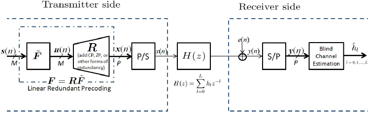
Figure 1: Block diagram of blind channel estimation in a redundant block transmission system

Theorem II.2.

Let $\bm{t}(\bm{y})$ be an unbiased estimator of an unknown parameter $\bm{\theta}\in\mathbb{C}^{n}$ based on observation $\bm{y}\in\mathbb{C}^{p}$ characterized by its pdf $p(\bm{y};\bm{\theta})$. Furthermore, we require the parameter $\bm{\theta}$ to satisfy a holomorphic constraint function $\bm{f}:\mathbb{C}^{n}\to\mathbb{C}^{m}$, $m\leq n$,

$$\bm{f}(\bm{\theta})=\bm{0}.$$ (6)

Assume that $\partial\bm{f}/\partial\bm{\theta}^{T}$ has full rank. Let $\bm{U}$ be a matrix with $(n-m)$ orthonormal columns that satisfies

$$\frac{\partial\bm{f}}{\partial\bm{\theta}^{T}}\bm{U}=\bm{0}.$$ (7)

Then

$$\mathsf{cov}\left(\bm{t},\bm{t}\right)\geq\bm{U}\left(\bm{U}^{H}\bm{J}\bm{U}\right)^{\dagger}\bm{U}^{H},$$ (8)

where $\bm{J}$ is the FIM defined as in (3). The equality holds if and only if

$$\bm{t}-\bm{\theta}=\bm{U}\left(\bm{U}^{H}\bm{J}\bm{U}\right)^{\dagger}\bm{U}^{H}\frac{\partial\ln p}{\partial\bm{\theta}^{*}}\quad\mbox{with probability }1.$$ (9)

Proof.

See Appendix B. ∎

With Theorem II.2, we are ready to derive the CRB for blind channel estimators in redundant block transmission systems, as shown in the following sections.

III System Model and Problem Formulation

In this section we formulate the blind channel estimation problem in a redundant block transmission system using an equivalent discrete-time baseband model.

The block diagram of a block transmission system is shown in Figure 1. Let the $n$th source block be expressed as an $M\times 1$ column vector

$$\bm{s}(n)=[\begin{array}[]{cccc}s_{0}(n)&s_{1}(n)&\cdots&s_{M-1}(n)\end{array}]^{T},$$ (10)

where each entry in the vector is a modulation symbol expressed as a complex value. The vector $\bm{s}(n)$ is precoded by a full-rank $M$-by-$M$ matrix $\tilde{\bm{F}}$ to obtain

$$\bm{u}(n)=\tilde{\bm{F}}\bm{s}(n).$$ (11)

In an OFDM system, $\tilde{\bm{F}}$ equals to $\bm{W}^{H}$, the normalized inverse discrete Fourier transform (IDFT) matrix; in a single carrier (SC) system, $\tilde{\bm{F}}$ equals to the identity matrix $\bm{I}_{M}$. We assume the general case that $\tilde{\bm{F}}$ is nonsingular as in [1]. For convenience we define

$$P\triangleq M+L.$$ (12)

The precoded $M$-vector $\bm{u}(n)$ is then added redundancy to obtain a $P$-vector

$$\bm{x}(n)=\bm{R}\bm{u}(n)$$

where $\bm{R}$ is a $P\times M$ full rank matrix representing the type of redundancy added. In a cyclic prefix (CP) system, we have

$$\bm{R}=\left[\begin{array}[]{cc}\bm{0}_{L\times(M-L)}&\bm{I}_{L}\\ \bm{I}_{M-L}&\bm{0}_{L}\\ \bm{0}_{L\times(M-L)}&\bm{I}_{L}\end{array}\right],$$ (13)

while in a ZP system, we have

$$\bm{R}=\left[\begin{array}[]{c}\bm{I}_{M}\\ \bm{0}_{L\times M}\end{array}\right].$$ (14)

In general, we have a unified expression for $\bm{x}(n)$,

$$\bm{x}(n)=\bm{R}\tilde{\bm{F}}\bm{s}(n)=\bm{F}\bm{s}(n)$$ (15)

where

$$\bm{F}\triangleq\bm{R}\tilde{\bm{F}}$$ (16)

is a full-rank $P\times M$ matrix. Note that ZP-OFDM, SC-ZP, CP-OFDM, and SC-CP systems are all special cases of the redundant block transmission system considered here.

After parallel-to-serial conversion, $\bm{x}(n)$ is sent to the channel, modeled as a finite impulse response (FIR) filter characterized by its $z$-transform

$$H(z)=\sum_{l=0}^{L}h_{l}z^{-l}.$$ (17)

The output of the FIR channel is the convolution of the input and the channel impulse response. Suppose the transmitter sends $N$ consecutive blocks defined as

$$\bm{s}_{N}\triangleq[\begin{array}[]{cccc}\bm{s}(0)^{T}&\bm{s}(1)^{T}&\ldots&\bm{s}(N-1)^{T}\end{array}]^{T}.$$ (18)

The $n$th received block, $\bm{y}(n)$, $n=0,1,2,...,N-1$, can be expressed as

$$\bm{y}(n)=\bm{H}_{1}\left[\begin{array}[]{c}\left[{\bm{x}}(n-1)\right]_{M+1:P}\\ \bm{x}(n)\\ \end{array}\right]+\bm{e}(n),$$ (19)

where $\bm{H}_{1}$ is a $P$-by-$(P+L)$ Toeplitz matrix [26] of the form

$$\bm{H}_{1}\triangleq\left[\begin{array}[]{ccccccc}h_{L}&\cdots&h_{1}&h_{0}&0&\cdots&0\\ 0&h_{L}&\cdots&h_{1}&h_{0}&\ddots&\vdots\\ \vdots&\ddots&\ddots&&\ddots&\ddots&0\\ 0&\cdots&0&h_{L}&\ddots&h_{1}&h_{0}\\ \end{array}\right],$$ (20)

and $\bm{e}(n)$ is the additive white Gaussian noise (AWGN) at the receiver side with zero mean and covariance matrix

$$\mathsf{E}[\bm{e}(n)\bm{e}^{H}(n)]=\sigma^{2}\bm{I}_{P}.$$ (21)

Notice that, for $n=0$, the values of the first $L$ entries of $\bm{y}(0)$ depend on undetermined vector $\bm{x}(-1)$. So for the channel estimation problem, we drop these $L$ samples from the observation and use only the last $M$ samples of the $0$th block $\bm{y}(0)$, which can be expressed as

$$[\bm{y}(0)]_{L+1:P}=\bm{H}_{2}\bm{x}(0)+\bm{e}(0)$$ (22)

where $\bm{H}_{2}$ is an $M\times P$ Toeplitz matrix of the same form as $\bm{H}_{1}$ in (20). Collect the $(NP-L)$ samples observed by the receiver and define the observation vector as

$$\bm{y}_{N}\triangleq[\begin{array}[]{cccc}[\bm{y}(0)]_{L+1:P}^{T}&\bm{y}(1)^{T}&\ldots&\bm{y}(N-1)^{T}\end{array}]^{T}.$$ (23)

Then it can be shown, from (15), (19), and (22), that

$$\bm{y}_{N}=\bm{G}\bm{H}(\bm{I}_{N}\otimes\bm{F})\bm{s}_{N}+\bm{e}_{N}$$ (24)

where

$$\bm{G}\triangleq\left[\begin{array}[]{ccc}\bm{0}_{(NP-L)\times L}&\bm{I}_{(NP-L)\times(NP-L)}&\bm{0}_{(NP-L\times L)}\end{array}\right],$$ (25)

$\bm{H}$ is a $(NP+L)$-by-$NP$ Toeplitz matrix of the form

$$\bm{H}\triangleq\left[\begin{array}[]{cccc}h_{0}&0&\cdots&0\\ h_{1}&\ddots&\ddots&\vdots\\ \vdots&\ddots&\ddots&0\\ h_{L}&\ddots&\ddots&h_{0}\\ 0&\ddots&\ddots&h_{1}\\ \vdots&\ddots&\ddots&\vdots\\ 0&\ldots&0&h_{L}\end{array}\right],$$ (26)

and the $(NP-L)$-vector $\bm{e}_{N}$ is defined as

$$\bm{e}_{N}\triangleq[\begin{array}[]{cccc}[\bm{e}(0)]_{L+1:P}^{T}&\bm{e}(1)^{T}&\ldots&\bm{e}(N-1)^{T}\end{array}]^{T}.$$ (27)

The product of matrices $\bm{G}$ and $\bm{H}$ defined above is actually equivalent to a matrix in a “fat” Toeplitz form as in (20). The reason we use this seemingly more complicated expression here is for convenience of CRB derivation, as will be shown later in the next section.

Now, the goal of blind channel estimation in a redundant block transmission system is to estimate

$$\bm{h}\triangleq\left[\begin{array}[]{cccc}h_{0}&h_{1}&\ldots&h_{L}\end{array}\right]^{T}$$ (28)

from the observation $\bm{y}_{N}$ defined in (23) and (24).

Although the problem studied here considers block transmission systems with all kinds of linearly redundant precoding including ZP systems, it should be noted that even when $\bm{R}$ is taken as the form in (14), the problem is slightly different from that defined in [1] due to the fact that the first $L$ entries of $\bm{y}(0)$ are not taken as part of the observation vector $\bm{y}_{N}$.

IV CRB for Blind Channel Estimators

We define the $(NM+L+1)$-fold parameter vector $\bm{\theta}$ as

$$\bm{\theta}\triangleq\left[\begin{array}[]{cc}\bm{h}^{T}&\bm{s}_{N}^{T}\end{array}\right]^{T},$$ (29)

where $\bm{s}_{N}$ is treated as a nuisance parameter [27]. To derive the CRB for blind channel estimators, we first identify the probability density function of the observation vector $\bm{y}_{N}$ given $\bm{\theta}$ and calculate the complex Fisher information matrix (FIM) $\bm{J}$ defined in (3). Then we apply Theorem II.2 to obtain the CRB expression in terms of $\bm{F},\bm{h},$ and $\bm{s}_{N}$.

By the assumption of additive white Gaussian noise, the probability density function of the receiver’s observation given $\bm{\theta}$ is

$$p(\bm{y}_{N};\bm{\theta})$$

$$\quad=\frac{1}{\left(\pi\sigma\right)^{NP-L}}\exp\left(-\frac{1}{\sigma^{2}}\left\|\bm{y}_{N}-\bm{G}\bm{H}\left(\bm{I}_{N}\otimes\bm{F}\right)\bm{s}_{N}\right\|^{2}\right).$$ (30)

The Toeplitz matrix $\bm{H}$ can be rewritten as

$$\bm{H}=\sum_{l=0}^{L}h_{l}\bm{J}_{l},$$ (31)

where the $(i,j)$th element of $\bm{J}_{l}$ is defined as

$$[\bm{J}_{l}]_{i,j}=\left\{\begin{array}[]{ll}1,&\mbox{ if }i-j=l\\ 0,&\mbox{ otherwise}\end{array},\right.l=0,1,...,L.$$ (32)

In the following derivations, for simplicity, we will use $\bm{K}$ and $\bm{K}_{l},l=0,1,...,L,$ to represent $\bm{K}\triangleq\bm{G}\bm{H}(\bm{I}_{N}\otimes\bm{F})$ and $\bm{K}_{l}\triangleq\bm{G}\bm{J}_{l}(\bm{I}_{N}\otimes\bm{F}),l=0,1,...,L,$ respectively. Note that $\bm{K}=\sum_{l=0}^{L}h_{l}\bm{K}_{l}.$ To calculate the FIM $\bm{J}$, we take partial derivatives on the logarithm probability density function with respect to elements of $\bm{\theta}$ and obtain the following equations.

$$\frac{\partial\ln p}{\partial h^{*}_{l}} =\dfrac{1}{\sigma^{2}}\bm{s}_{N}^{H}(\bm{I}_{N}\otimes\bm{F})^{H}\bm{J}_{l}^{H}\bm{G}^{H}$$

$$\quad\left[\bm{y}_{N}-\bm{G}\bm{H}(\bm{I}_{N}\otimes\bm{F})\bm{s}_{N}\right]$$

$$=\dfrac{1}{\sigma^{2}}\bm{s}_{N}^{H}\bm{K}_{l}^{H}\bm{e}_{N}.$$ (33)

$$\frac{\partial\ln p}{\partial h_{l}} =\left(\frac{\partial\ln p}{\partial h^{*}_{l}}\right)^{*}.$$ (34)

$$\frac{\partial\ln p}{\partial\bm{s}_{N}^{*}} =\frac{1}{\sigma^{2}}(\bm{I}_{N}\otimes\bm{F})^{H}\bm{H}^{H}\bm{G}^{H}$$

$$\quad\left[\bm{y}_{N}-\bm{G}\bm{H}(\bm{I}_{N}\otimes\bm{F})\bm{s}_{N}\right]$$

$$=\frac{1}{\sigma^{2}}\bm{K}^{H}\bm{e}_{N}.$$ (35)

$$\frac{\partial\ln p}{\partial\bm{s}_{N}} =\left(\frac{\partial\ln p}{\partial\bm{s}_{N}^{*}}\right)^{*}$$ (36)

Now, divide $\bm{J}$ into $4$ sub-matrices

$$\bm{J}=\mathsf{E}\left[\left(\frac{\partial\ln p}{\partial\bm{\theta^{*}}}\right)\left(\frac{\partial\ln p}{\partial\bm{\theta^{*}}}\right)^{H}\right]\triangleq\left[\begin{array}[]{cccc}\bm{J}_{0,0}&\bm{J}_{0,1}\\ \bm{J}_{1,0}&\bm{J}_{1,1}\\ \end{array}\right].$$ (39)

The entries of these sub-matrices can be written as

$$[\bm{J}_{0,0}]_{i,j} \triangleq\mathsf{E}\left[\frac{\partial\ln p}{\partial h^{*}_{i}}\frac{\partial\ln p}{\partial h_{j}}\right],$$ (40)

$$[\bm{J}_{0,1}]_{i,j} \triangleq\mathsf{E}\left[\frac{\partial\ln p}{\partial h^{*}_{i}}\frac{\partial\ln p}{\partial[\bm{s}_{N}]_{j}}\right],$$ (41)

$$[\bm{J}_{1,0}]_{i,j} \triangleq\mathsf{E}\left[\frac{\partial\ln p}{\partial[\bm{s}_{N}^{*}]_{i}}\frac{\partial\ln p}{\partial h_{j}}\right],$$ (42)

and

$$[\bm{J}_{1,1}]_{i,j} \triangleq\mathsf{E}\left[\frac{\partial\ln p}{\partial[\bm{s}_{N}^{*}]_{i}}\frac{\partial\ln p}{\partial[\bm{s}_{N}]_{j}}\right],$$ (43)

respectively. By equations (33, 34, 35, 36) and the fact that $\mathsf{E}[\bm{e}_{N}\bm{e}_{N}^{H}]=\sigma^{2}\bm{I}_{NP-L}$, we have the following results.

1. For the sub-matrix $\bm{J}_{0,0}$:

   $$[\bm{J}_{0,0}]_{i,j}=\frac{1}{\sigma^{2}}\bm{s}_{N}^{H}\bm{K}_{i}^{H}\bm{K}_{j}\bm{s}_{N}.$$ (44)

   Therefore, we can write $\bm{J}_{0,0}$ as

   $$\bm{J}_{0,0} =\frac{1}{\sigma^{2}}\left[\begin{array}[]{c}\bm{s}_{N}^{H}\bm{K}_{0}^{H}\\ \vdots\\ \bm{s}_{N}^{H}\bm{K}_{L}^{H}\end{array}\right]\left[\begin{array}[]{c}\bm{s}_{N}^{H}\bm{K}_{0}^{H}\\ \vdots\\ \bm{s}_{N}^{H}\bm{K}_{L}^{H}\end{array}\right]^{H}.$$ (51)

2. For the sub-matrix $\bm{J}_{0,1}$, the $i$th row of $\bm{J}_{0,1}$ is

   $$\mathsf{E}\left[\frac{\partial\ln p}{\partial h^{*}_{i}}\left(\frac{\partial\ln p}{\partial\bm{s}_{N}}^{T}\right)\right] =\frac{1}{\sigma^{2}}\bm{s}_{N}^{H}\bm{K}_{i}^{H}\bm{K}.$$ (52)

   Therefore,

   $$\bm{J}_{0,1}=\frac{1}{\sigma^{2}}\left[\begin{array}[]{c}\bm{s}_{N}^{H}\bm{K}_{0}^{H}\bm{K}\\ \vdots\\ \bm{s}_{N}^{H}\bm{K}_{L}^{H}\bm{K}\end{array}\right].$$ (53)

3. For the sub-matrix $\bm{J}_{1,0}$, we have

   $$\bm{J}_{1,0}=\bm{J}_{0,1}^{H}.$$ (54)

4. For the sub-matrix $\bm{J}_{1,1}$, we have

   $$\bm{J}_{1,1} =\mathsf{E}\left[\frac{\partial\ln p}{\partial\bm{s}_{N}^{*}}\left(\frac{\partial\ln p}{\partial\bm{s}_{N}^{*}}\right)^{H}\right]=\frac{1}{\sigma^{2}}\bm{K}^{H}\bm{K}.$$ (55)

Since $\bm{\theta}=[\begin{array}[]{cc}\bm{h}^{T}&\bm{s}_{N}^{T}\end{array}]^{T}$ and $\bm{\theta}^{\prime}\triangleq[\begin{array}[]{cc}(1/c)\bm{h}^{T}&c\bm{s}_{N}^{T}\end{array}]^{T}$ will result in the same observation vector $\bm{y}$ for any nonzero $c\in\mathbb{C}$, an unbiased blind channel estimator will not exist. This is commonly known as the scalar ambiguity issue and is usually resolved by setting one element in $\bm{\theta}$ as already known [1]. Here we follow the approach in [1] that we assume the $d$th element of $\bm{h}$, $h_{d}$, is nonzero and already known to the receiver. In the perspective of CRB for constrained parameters, this assumption corresponds to the constraint function

$$f(\bm{\theta})=h_{d}-h_{d}^{0},$$ (56)

where $h_{d}^{0}$ is the realized value of $h_{d}$. Obviously $f$ is a holomorphic map. We can then apply Theorem II.2 and obtain the CRB with the constraint function $f$ as

$$\mathsf{cov}(\bm{\theta},\bm{\theta})\geq\bm{E}_{d}^{\prime H}\left(\bm{E}_{d}^{\prime}\bm{J}\bm{E}_{d}^{\prime H}\right)^{-1}\bm{E}_{d}^{\prime},$$ (57)

where $\bm{E}_{d}^{\prime}$ is obtained by removing the $d$th row of $\bm{I}_{NM+L+1}$, the identity matrix of order $(NM+L+1)$ (Note that $\bm{E}_{d}^{\prime}$ satisfies (7)). All elements on the $d$th row and $d$th column of (57) are zero, implying the $d$th parameter, $h_{d}$, always has a zero MSE, consistent with the fact that the receiver has a priori information $\hat{h_{d}}=h_{d}^{0}$. Therefore we ignore the $d$th row and column of (57) and only consider the covariance bound for estimators of $\bm{\theta}_{d}\triangleq[h_{0},\ldots,h_{d-1},h_{d+1},\ldots,h_{L},\bm{s}_{N}^{T}]^{T}$, (i.e., $\left(\bm{E}_{d}^{\prime}\bm{J}\bm{E}_{d}^{\prime H}\right)^{-1}$) in the following discussion. Let $\tilde{\bm{J}}\triangleq\bm{E}_{d}^{\prime}\bm{J}\bm{E}_{d}^{\prime H}$. Then the matrix $\tilde{\bm{J}}$ is of the form

$$\tilde{\bm{J}}\triangleq\left[\begin{array}[]{cc}\bm{E}_{d}\bm{J}_{0,0}\bm{E}_{d}^{H}&\bm{E}_{d}\bm{J}_{0,1}\\ \bm{J}_{0,1}^{H}\bm{E}_{d}^{H}&\bm{J}_{1,1}\end{array}\right]$$ (58)

where $\bm{E}_{d}$ is an $L\times(L+1)$ matrix obtained by removing the $d$th row from $\bm{I}_{L+1}$. Then, equation (57) implies that for any unbiased estimator $\hat{\bm{\theta}_{d}}$ of $\bm{\theta}_{d}$,

$$\mathsf{cov}\left(\hat{\bm{\theta}_{d}},\hat{\bm{\theta}_{d}}\right)\geq\tilde{\bm{J}}^{-1}.$$ (59)

Since we only focus on the performance of channel estimators, we can simplify the above equation to obtain a bound for $\mathsf{cov}(\hat{\bm{h}_{d}},\hat{\bm{h}_{d}})$, where $\bm{h}_{d}\triangleq[h_{0},...,h_{d-1},h_{d+1},...,h_{L}]$. This can be done by noting that (59) implies

$$\left[\begin{array}[]{cc}\bm{I}_{L}&\bm{0}_{L\times NM}\end{array}\right]\mathsf{cov}\left(\hat{\bm{\theta}_{d}},\hat{\bm{\theta}_{d}}\right)\left[\begin{array}[]{c}\bm{I}_{L}^{H}\\ \bm{0}_{L\times NM}^{H}\end{array}\right]\geq$$ (63)

$$\quad\quad\quad\quad\quad\quad\left[\begin{array}[]{cc}\bm{I}_{L}&\bm{0}_{L\times NM}\end{array}\right]\tilde{\bm{J}}^{-1}\left[\begin{array}[]{c}\bm{I}_{L}^{H}\\ \bm{0}_{L\times NM}^{H}\end{array}\right].$$ (67)

The left side of the inequality corresponds to the covariance matrix of $\bm{h}_{d}$. Therefore, the CRB for any unbiased estimator $\hat{\bm{h}_{d}}$, of $\bm{h}_{d}$, can be calculated as the upper-left $L$-by-$L$ sub-matrix of $\tilde{\bm{J}}^{-1}$:

$$\bm{C}_{\mathrm{CRB}}\triangleq\left[\bm{E}_{d}\left(\bm{J}_{0,0}-\bm{J}_{0,1}\bm{J}_{1,1}^{-1}\bm{J}_{0,1}^{H}\right)\bm{E}_{d}^{H}\right]^{-1}.$$ (68)

$$\bm{C}_{\mathrm{CRB}}(\bm{h},\bm{s}_{N},\bm{F},d)=\sigma^{2}\left(\bm{E}_{d}\ \tilde{\mathcal{U}}\left\{\bm{I}_{(N-1)L}\otimes\left[(\bm{I}_{N}\otimes\bm{F})^{*}\bm{s}_{N}^{*}\bm{s}_{N}^{T}(\bm{I}_{N}\otimes\bm{F})^{T}\right]\right\}\tilde{\mathcal{U}}^{H}\ \bm{E}_{d}^{H}\right)^{-1}.$$ (69)

From Appendix C, we obtain the final form of the CRB for blind channel estimation in any given redundant block transmission systems, as shown in (69), in terms of $\bm{h}$, $\bm{s}_{N}$, $d$, and $\bm{F}$. In (69), the matrix $\tilde{\cal U}$ has a size of $(L+1)\times LPN(N-1)$ and can be determined by vector $\bm{h}$ and matrix $\bm{F}$. The values of nonzero entries of $\tilde{{\cal U}}$ all come from the $(N-1)L$ orthonormal left annihilators of $\bm{K}=\bm{G}\bm{H}(\bm{I}_{N}\otimes\bm{F})$ and are defined in details in (115).

Although the CRB considers all LRP, including ZP systems (i.e., $\bm{F}$ satisfies (16)(14)), the CRB expression in (69) does not reduce to that obtained in [1, 2] in this situation. The reason is that in the derivation of this CRB, we do not use the first $L$ entries of the first block as part of the observation vector. In fact, as will be shown in Section V, with a smaller observation vector, the CRB values derived here are expected to be slightly higher than those derived in [1, 2].

V Numerical Results

In this section we first compare the performance of existing blind channel estimation algorithms for CP systems with the CRBs derived in this paper. The subspace-based blind channel estimators proposed in [3, 9] are chosen as benchmarks.

The simulation settings are concluded in Table I. The simulation results are averaged over $N_{ch}=500$ independent channel realizations. All elements in the $i$th realization of $\bm{h}$, defined as $\bm{h}^{(i)}=[\begin{array}[]{cccc}h_{0}^{(i)}&h_{1}^{(i)}&\cdots&h_{L}^{(i)}\end{array}]$, are generated first as independent complex Gaussian random variables with zero mean and unity variance and then normalized to satisfy $\|\bm{h}^{(i)}\|^{2}=1$. For each channel realization, $N_{s}=30$ trials with independent sets of QPSK modulated data symbols are conducted to further average the channel estimation MSE, defined as:

$$\mbox{MSE}\triangleq{1\over N_{ch}N_{s}}\sum_{i=1}^{N_{ch}}\sum_{j=1}^{N_{s}}\|(h_{d_{i}}^{(i)}/\hat{h}^{(i,j)}_{d_{i}})\hat{\bm{h}}^{(i,j)}-\bm{h}^{(i)}\|^{2},$$ (70)

where $\hat{\bm{h}}^{(i,j)}$ is the estimate of the $i$th channel realization in the $j$th trial, and $d_{i}$ is chosen as the index of the channel tap with the maximal power: $d_{i}=\arg\max_{0\leq d\leq L}\left|h_{d}^{(i)}\right|^{2}.$ Similarly, the CRB curves are calculated according to

$$\mbox{CRB}\triangleq{1\over N_{ch}N_{s}}\sum_{i=1}^{N_{ch}}\sum_{j=1}^{N_{s}}\mathsf{tr}\left[{\bm{C}_{\mathrm{CRB}}(\bm{h}^{(i)},\bm{s}_{N}^{(i,j)},\bm{F},d_{i})}\right]$$ (71)

with the same channel and data set realizations.

TABLE I: Simulation Settings for CP Systems

Block size $M$	12
Number of received blocks $N$	8, 25, 50
Channel order $L$	4
Modulation	QPSK

Figure 2: CRB and simulatoin results for SC-CP system with 25 blocks

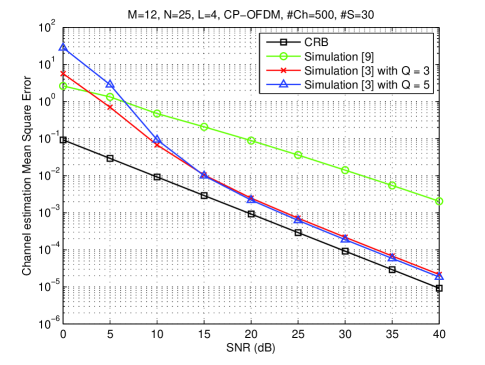
Figure 3: CRB and simulatoin results for OFDM-CP system with 25 blocks

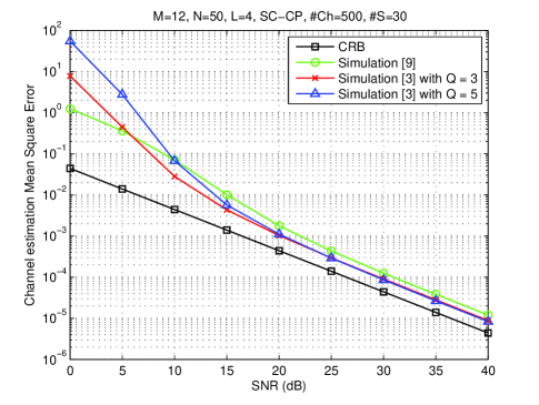
Figure 4: CRB and simulatoin results for SC-CP system with 50 blocks

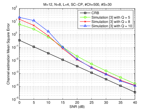
Figure 5: CRB and simulatoin results for SC-CP system with 8 blocks

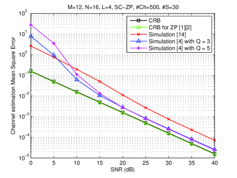
Figure 6: CRB and simulatoin results for SC-ZP system

We first consider the blind channel estimation problem in SC-CP ($\tilde{\bm{F}}=\bm{I}_{M}$, $\bm{R}$ is chosen as in (13)) systems with 25 received blocks available. The performance of algorithms proposed in [3] and [9], as well as the CRB derived in this paper, are depicted in Figure 2. We can see the algorithm in [3] has advantage over that in [9] in high-SNR region while the algorithm in [9] has better performance with a low SNR. As predicted in [3], increasing the algorithm parameter $Q$ from 3 to 5 gains a slight MSE improvement in high SNR region but results in a large performance degradation when SNR is low. Under high SNR values, for both curves of algorithms[3], the gap between the simulation MSE result and the CRB, tends to approach a constant in log scale (around 3 to 4 dB in SNR). All these MSE results do not achieve the performance lower bound suggested by the CRB.

Figure 3 considers CP-OFDM systems (i.e., $\tilde{\bm{F}}=\bm{W}^{H}$)with the same simulation settings. The performance curves are almost identical to those in Figure 2. This suggests the precoder $\tilde{\bm{F}}$ does not significantly affect the MSE and CRB curves for blind channel estimators in CP systems. All following simulations will then consider single carrier systems only.

In Figure 4, we consider the problem in SC-CP systems with 50 received blocks. The MSE and CRB curves are all lower than those in previous plots. The gaps between the CRB and MSE results still converge to constant values in log scale in the high-SNR region. For both curves of algorithm [3], the gap is around 3 dB; for algorithm [9], it is around 5dB.

The case with only 8 available received blocks is studied in Figure 5. As algorithm in [9] does not work appropriately with such a small amount of received data, only performance curves of algorithm in [3], with large values of $Q$, are presented. We observe that performance in the high-SNR region improves when the algorithm parameter $Q$ is chosen as a large value. But the improvement slows down gradually as $Q$ increases to 10. Similarly, it results in performance degradation with low SNR values. For the high SNR region, in the best situation shown ($Q=10$), the gap between the MSE performance and the CRB is around 4 to 5 dB in high SNR region.

We now turn our attention to ZP systems (i.e., $\bm{F}$ satisfies (16)(14)). We compared the derived CRB, CRB reported in [1, 2], and MSE performances of existing blind algorithms [4, 14] in Figure 6. In Figure 6, our CRB is slightly higher than that reported in [1, 2], with a margin of less than 0.5dB. This is consistent with the fact that the first $L$ entries of the first block are dropped from the observation vector (as stated at the end of Sections III and IV). This discrepancy in two CRBs, however, is much smaller than the gap between MSE performances of existing algorithms and the CRBs. The generalized algorithm in [4] has a performance gap to the CRB of around 2 dB in high SNR region. The performance curve of an earlier method in [14] is around 7dB from the CRB bound.

Summarizing all above simulation results, in both CP and ZP systems, all existing blind channel estimation algorithms [9, 3, 14, 4] do not achieve the lower bound suggested by CRB. In the high-SNR region, the generalized subspace methods proposed in [4] [3] obtain the best performances among others, regardless of the number of available received blocks. But a gap of around 2 to 4 dB from the best performance to the CRB is constantly present, suggesting there is still room for performance improvement of blind channel estimators in these systems.

VI Conclusions and Future Work

In this paper, we derived the CRB for blind channel estimators in redundant block transmission systems. The derived CRB is valid for any full-rank linear redundant precoder (LRP), including both ZP and CP systems and is an extension to the result in [1, 2]. We compared the derived CRB with the performances of the existing subspace-based blind channel estimators for CP [3, 9] and ZP systems [14, 4]. Numerical results show that these existing blind channel estimators for ZP and CP systems do not achieve the CRB and there is still some room for performance improvement.

In addition, a simple form of CRB formula is derived for unconstrained and constrained complex parameters. We extended this form, originally for real parameters[15, 16, 17], to the case of multiple complex parameters. The results not only facilitate the derivation of CRB for the blind channel estimation problem of interest, but also are expected to be useful for other complex CRB derivations.

In the future, there are a few research directions worthy of being explored. The CRB derived in this paper is applicable to blind channel estimators which do not have a priori information about the transmitted signals. It would be desirable to derive the CRB for blind channel estimator that assume some stronger assumptions about the transmitted signals. For example, the receiver should know the modulation scheme the transmitter uses, which corresponds to the finite alphabet assumption [10]. One possible approach for this is to use the CRB for constrained complex parameters. Take quadrature phase-shift keying (QPSK) for example. The finite-alphabet assumption that QPSK is used can be modeled by setting the constraint function as $\bm{f}(\bm{\theta})=[\begin{array}[]{cccc}s_{0}(0)^{4}&s_{1}(0)^{4}&\ldots&s_{M-1}(N-1)^{4}\end{array}]^{T}-[\begin{array}[]{cccc}1&1&\ldots&1\end{array}]^{T}$, assuming each modulation symbol has unit power. It is obvious that $\bm{f}$ is holomorphic, so Theorem II.2 can be applied. This approach, however, cannot be directly extended to more complex modulation schemes such as 16-quadrature amplitude modulation (16-QAM). And this will require additional research efforts.

Furthermore, the receiver may, in additional to the modulation scheme, also know the joint probability distribution of the transmitted symbols. The CRB for this case, at first glance, can be derived by Bayesian Cramér-Rao bound (BCRB), or Van Trees inequality [17, 28]. BCRB is a lower bound of variance for all estimators knowing the a priori distribution of the unknown parameters. The BCRB, however, cannot be applied to discrete parameters, such as modulation symbols. An extension of the original BCRB formula to discrete parameters or a new bound for such cases is desirable.

Appendix A Proof of Theorem II.1

In order to prove Theorem II.1, we apply the following lemma analogous to the well-known Cauchy-Schwartz inequality, which can be considered as the Cauchy-Schwartz inequality for random vectors. Although this lemma has been already proved in [15, 23], we show the proof here because it helps illustrate the necessary and sufficient condition of when the equality of CRB holds.

Lemma A.1.

For any two random vectors $\bm{x},\bm{y}\in\mathbb{F}^{n}$, where $\mathbb{F}$ can be $\mathbb{R}$ or $\mathbb{C}$,

$$\mathsf{cov}(\bm{y},\bm{y})\geq\mathsf{cov}(\bm{y},\bm{x})\mathsf{cov}(\bm{x},\bm{x})^{\dagger}\mathsf{cov}(\bm{x},\bm{y}).$$ (72)

Proof.

The proof presented here is from [23]. Define

$$\begin{array}[]{ll}\bm{\Sigma}_{11}\triangleq\mathsf{cov}(\bm{x},\bm{x}),&\bm{\Sigma}_{12}\triangleq\mathsf{cov}(\bm{x},\bm{y}),\\ \bm{\Sigma}_{21}\triangleq\mathsf{cov}(\bm{y},\bm{x}),&\bm{\Sigma}_{22}\triangleq\mathsf{cov}(\bm{y},\bm{y}).\end{array}$$ (73)

Define a random vector $\bm{z}\triangleq\bm{y}-\bm{\Sigma}_{21}\bm{\Sigma}_{11}^{\dagger}\bm{x}$, then we have

$$\mathsf{cov}(\bm{z},\bm{z}) =\bm{\Sigma}_{22}-\bm{\Sigma}_{21}\left(\bm{\Sigma}_{11}^{\dagger}\right)^{H}\bm{\Sigma}_{21}^{H}-\bm{\Sigma}_{21}\bm{\Sigma}_{11}^{\dagger}\bm{\Sigma}_{12}$$ (74)

$$\quad+\bm{\Sigma}_{21}\bm{\Sigma}_{11}^{\dagger}\bm{\Sigma}_{11}\left(\bm{\Sigma}_{11}^{\dagger}\right)^{H}\bm{\Sigma}_{21}^{H}$$

$$=\bm{\Sigma}_{22}-\bm{\Sigma}_{21}\bm{\Sigma}_{11}^{\dagger}\bm{\Sigma}_{12}.$$ (75)

The second equality follows by $\left(\bm{A}^{\dagger}\right)^{H}=\left(\bm{A}^{H}\right)^{\dagger}$ and $\bm{A}^{\dagger}\bm{A}\bm{A}^{\dagger}=\bm{A}^{\dagger}$ for any matrix $\bm{A}$.

The lemma follows since any covariance matrix is nonnegative definite. ∎

Now we are ready to prove Theorem II.1, a CRB for unconstrained complex parameters.

Proof of Theorem II.1:

Proof.

Since $\bm{t}$ is an unbiased estimator,

$$\mathsf{E}\left[\bm{t}(\bm{y})\right]=\bm{\theta}.$$ (76)

Differentiate both sides with respect to $\bm{\theta}^{T}$, we can get

$$\int\bm{t}(\bm{y})\frac{\partial p}{\partial\bm{\theta}^{T}}\ d\bm{y}=\bm{I}_{n};$$ (77)

equivalently,

$$\int\bm{t}(\bm{y})\frac{\partial\ln p}{\partial\bm{\theta}^{T}}p\ d\bm{y}=\bm{I}_{n}.$$ (78)

With the regularity condition we can rewrite (78) as

$$\mathsf{cov}\left(\bm{t},\frac{\partial\ln p}{\partial\bm{\theta}^{*}}\right)=\bm{I}_{n}.$$ (79)

Now, substitute $\bm{x}$ and $\bm{y}$ in (72) by $(\partial\ln p)/(\partial\bm{\theta}^{*})$ and $\bm{t}$, respectively, we have

$$\quad\mathsf{cov}\left(\bm{t},\bm{t}\right)$$

$$\geq\mathsf{cov}\left(\bm{t},\frac{\partial\ln p}{\partial\bm{\theta}^{*}}\right)\mathsf{cov}\left(\frac{\partial\ln p}{\partial\bm{\theta}^{*}},\frac{\partial\ln p}{\partial\bm{\theta}^{*}}\right)^{\dagger}\mathsf{cov}\left(\bm{t},\frac{\partial\ln p}{\partial\bm{\theta}^{*}}\right)^{H}$$

$$=\mathsf{cov}\left(\frac{\partial\ln p}{\partial\bm{\theta}^{*}},\frac{\partial\ln p}{\partial\bm{\theta}^{*}}\right)^{\dagger}$$

$$=\mathsf{E}\left[\left(\frac{\partial\ln p}{\partial\bm{\theta}^{*}}\right)\left(\frac{\partial\ln p}{\partial\bm{\theta}^{*}}\right)^{H}\right]^{\dagger}=\bm{J}^{\dagger}.$$ (80)

The first equality follows by (79), and the second equality follows by the regularity condition.

As for the necessary and sufficient condition of the equality, from the proof for Lemma A.1, we have $\mathsf{cov}(\bm{z},\bm{z})=\bm{0}$ if and only if $\bm{z}=\bm{c}$ with probability $1$ for some constant vector $\bm{c}$, that is,

$$\bm{t}-\bm{J}^{\dagger}\frac{\partial\ln p}{\partial\bm{\theta}^{*}}=\bm{c}.$$ (81)

Taking expectation on the both sides of the equality, by the regularity condition, we have

$$\mathsf{E}\left[\bm{t}\right]=\bm{c}.$$ (82)

Since $\bm{t}$ is unbiased, $\bm{c}=\bm{\theta}$.∎

$$\bm{D} =\frac{1}{\sigma^{2}}\left\{\bm{I}_{L+1}\otimes\bm{x}_{N}^{H}\right\}\left[\begin{array}[]{ccc}\mathsf{vec}(\tilde{\mathcal{U}}_{0})&\ldots&\mathsf{vec}(\tilde{\mathcal{U}}_{(N-1)L-1})\end{array}\right]\left[\begin{array}[]{ccc}\mathsf{vec}(\tilde{\mathcal{U}}_{0})&\ldots&\mathsf{vec}(\tilde{\mathcal{U}}_{(N-1)L-1})\end{array}\right]^{H}\left\{\bm{I}_{L+1}\otimes\bm{x}_{N}\right\}.$$ (85)

$$\bm{D} =\frac{1}{\sigma^{2}}\left[\begin{array}[]{ccc}\mathsf{vec}\left(\bm{x}_{N}^{H}\tilde{\mathcal{U}}_{0}\right)&\ldots&\mathsf{vec}\left(\bm{x}_{N}^{H}\tilde{\mathcal{U}}_{(N-1)L-1}\right)\end{array}\right]\left[\begin{array}[]{ccc}\mathsf{vec}\left(\bm{x}_{N}^{H}\tilde{\mathcal{U}}_{0}\right)&\ldots&\mathsf{vec}\left(\bm{x}_{N}^{H}\tilde{\mathcal{U}}_{(N-1)L-1}\right)\end{array}\right]^{H}.$$ (88)

Appendix B Proof of Theorem II.2

To prove Theorem II.2, we first derive some lemmas for holomorphic maps. First of all, the lemma of implicit functions is presented below.

Lemma B.1.

Let $B\subset\mathbb{C}^{n}\times\mathbb{C}^{m}$ be an open set, $\bm{f}:B\to\mathbb{C}^{m}$ a holomorphic map, $(\bm{z}_{0},\bm{w}_{0})\in B$ a point with $\bm{f}(\bm{z}_{0},\bm{w}_{0})=\bm{0}$, and

$$\mathsf{det}\left(\frac{\partial\bm{f}}{\partial[w_{1},\ldots,w_{m}]}(\bm{z}_{0},\bm{w}_{0})\right)\neq 0.$$ (83)

Then there is an open neighborhood $U=U^{\prime}\times U^{\prime\prime}\subset B$ and a holomorphic map $\bm{g}:U^{\prime}\to U^{\prime\prime}$ such that

$$\{(\bm{z},\bm{w})\in U^{\prime}\times U^{\prime\prime}:\bm{f}(\bm{z},\bm{w})=\bm{0}\}=\{(\bm{z},\bm{g}(\bm{z})):\bm{z}\in U^{\prime}\}.$$ (84)

Proof.

See [22]. ∎

Now consider the case where the possible values of $\bm{\theta}$ is constrained to a set $\Theta\triangleq\left\{\bm{\theta}\in\mathbb{C}^{n}:\bm{f}(\bm{\theta})=\bm{0}\right\}$ defined by a holomorphic constraint function $\bm{f}:\mathbb{C}^{n}\to\mathbb{C}^{m}$, $m\leq n$. Available observation is $\bm{y}\in\mathbb{C}^{p}$ with pdf $p(\bm{y};\bm{\theta})$. The goal here is to derive the CRB for any unbiased estimator $\bm{t}(\bm{y})$ of $\bm{\theta}$. Note now the unbiasedness refers to

$$\mathsf{E}\left[\bm{t}(\bm{y})\right]=\bm{\theta}$$ (85)

for all $\bm{\theta}\in\Theta$ instead of the whole $\mathbb{C}^{n}$. Assume $\partial\bm{f}/\partial\bm{\theta}^{T}$ has full rank for all $\bm{\theta}\in\Theta$ so Lemma B.1 applies. Then, we have the following lemma.

Lemma B.2.

Let $\bm{t}(\bm{y})$ be an unbiased estimator of $\bm{\theta}$ for all $\bm{\theta}\in\Theta$. Then

$$\mathsf{E}\left[\left(\bm{t}-\bm{\theta}\right)\frac{\partial\ln p(\bm{y};\bm{\theta})}{\partial\bm{\theta}^{T}}\right]\bm{\delta}=\bm{\delta}$$ (86)

for all $\bm{\theta}\in\Theta$, and $\bm{\delta}$ such that

$$\frac{\partial\bm{f}}{\partial\bm{\theta}^{T}}\bm{\delta}=\bm{0}.$$ (87)

Proof.

Follow the derivation of [25, Theorem I]. Note that the implicit function theorem and chain rule hold for holomorphic constraint functions [22]. ∎

And a corollary immediately follows.

Corollary B.1.

Choose a matrix $\bm{U}$ with orthonormal columns such that

$$\frac{\partial\bm{f}}{\partial\bm{\theta}^{T}}\bm{U}=\bm{0}.$$ (88)

Then

$$\mathsf{E}\left[\left(\bm{t}-\bm{\theta}\right)\frac{\partial\ln p(\bm{y};\bm{\theta})}{\partial\bm{\theta}^{T}}\right]\bm{U}=\bm{U}.$$ (89)

Proof.

Note that every column of $\bm{U}$ satisfies (87). ∎

Now we are ready to prove Theorem II.2.

Proof.

Substitute $\bm{x}$ and $\bm{y}$ in (72) by $\bm{U}^{H}(\partial\ln p)/(\partial\bm{\theta}^{*})$ and $\bm{t}$, respectively. Then apply Corollary B.1 to simplify the equation. As in the proof for Theorem II.1, the equality holds if and only if

$$\bm{t}-\bm{U}\left(\bm{U}^{H}\bm{J}\bm{U}\right)^{\dagger}\bm{U}^{H}\frac{\partial\ln p}{\partial\bm{\theta}^{*}}=\bm{c}\quad\mbox{with probability }1$$ (90)

for some constant vector $\bm{c}$. Taking expectations on both sides of (90) and we have $\bm{c}=\bm{\theta}$. ∎

Appendix C Proof of CRB

In this appendix, we show how to derive the CRB from (68) to the final form (69). Define $\bm{A}\triangleq\bm{J}_{0,1}\bm{J}_{1,1}^{-1}\bm{J}_{0,1}^{H}$. Then, using equations (53) and (55), the $(i,j)$th element of $\bm{A}$ can be calculated as

$$[\bm{A}]_{i,j}= \frac{1}{\sigma^{2}}\bm{s}_{N}^{H}\bm{K}_{i}^{H}\bm{K}\bm{K}^{\dagger}\bm{K}_{j}\bm{s}_{N}.$$ (91)

Define $\bm{D}\triangleq\bm{J}_{0,0}-\bm{J}_{0,1}\bm{J}_{1,1}^{-1}\bm{J}_{0,1}^{H}$. Then we have, by (51) and (91),

$$[\bm{D}]_{i,j}= {1\over\sigma^{2}}\bm{s}_{N}^{H}\bm{K}_{i}^{H}\left(\bm{I}_{NP-L}-\bm{K}\bm{K}^{\dagger}\right)\bm{K}_{j}\bm{s}_{N}.$$ (92)

By assumption, $\tilde{\bm{F}}$ is a full-rank matrix, and thus $\bm{F}$ is a full-column-rank matrix. The singular value decomposition (SVD) of the matrix $\bm{K}=\bm{G}\bm{H}(\bm{I}_{N}\otimes\bm{F})$, therefore, is of the form

$$\quad\bm{K}=\bm{G}\bm{H}(\bm{I}_{N}\otimes\bm{F})=\left[\begin{array}[]{cc}\bar{\bm{U}}&\tilde{\bm{U}}\end{array}\right]\left[\begin{array}[]{c}\bm{\Sigma}\\ \bm{0}\end{array}\right]\bm{V}^{H},$$ (96)

in which the matrix $\tilde{\bm{U}}$ represents the null space and has a size of $(NP-L)\times(NL-L)$. Now, we have

$$\bm{I}_{NP-L}-\bm{K}\bm{K}^{\dagger}=\tilde{\bm{U}}\tilde{\bm{U}}^{H},$$ (97)

and we can rewrite $[\bm{D}]_{i,j}$ in (92) as

$$[\bm{D}]_{i,j}=\frac{1}{\sigma_{2}}\bm{x}_{N}^{H}\bm{J}_{i}^{H}\bm{G}^{H}\tilde{\bm{U}}(\bm{G}\tilde{\bm{U}})^{H}\bm{J}_{j}\bm{x}_{N}$$ (98)

where

$$\bm{x}_{N}\triangleq\bm{s}_{N}^{H}(\bm{I}_{N}\otimes\bm{F})^{H}$$ (99)

is the vector containing precoded transmitted symbols. Now, we can express $\bm{D}$ as

$$\bm{D}= \frac{1}{\sigma^{2}}\left(\bm{I}_{L+1}\otimes\bm{x}_{N}^{H}\right)\left[\begin{array}[]{c}\bm{J}_{0}^{H}\bm{G}^{H}\tilde{\bm{U}}\\ \vdots\\ \bm{J}_{L}^{H}\bm{G}^{H}\tilde{\bm{U}}\end{array}\right]\left[\begin{array}[]{c}\bm{J}_{0}^{H}\bm{G}^{H}\tilde{\bm{U}}\\ \vdots\\ \bm{J}_{L}^{H}\bm{G}^{H}\tilde{\bm{U}}\end{array}\right]^{H}$$ (106)

$$\cdot\left(\bm{I}_{L+1}\otimes\bm{x}_{N}\right).$$

Define the Hankel matrix

$$\tilde{\mathcal{U}}_{j}\triangleq\left[\begin{array}[]{cccc}u_{0,j}&u_{1,j}&\ldots&u_{L,j}\\ u_{1,j}&u_{2,j}&\ldots&u_{L+1,j}\\ \vdots&\vdots&\ddots&\vdots\\ u_{PN-1,j}&u_{PN,j}&\ldots&u_{PN+L-1,j}\end{array}\right],$$ (107)

where $u_{i,j}$ denotes the $(i,j)$th element of the matrix $\bm{G}^{H}\tilde{\bm{U}}$. Notice that $u_{i,j}=0$ for $0\leq i\leq L-1$ and $PN\leq i\leq PN+L-1$ due to the structure of matrix $\bm{G}$. The matrix $\bm{D}$ can then be written as in (85). Noting that $\left(\bm{B}^{T}\otimes\bm{A}\right)\mathsf{vec}\left(\bm{X}\right)=\mathsf{vec}\left(\bm{A}\bm{X}\bm{B}\right)$ for any three matrices $\bm{A}$, $\bm{B}$, and $\bm{X}$ [26], we have (88). Since $\bm{x}_{N}^{H}\tilde{\mathcal{U}}_{i}$ is only a row vector for all $i$, the above equation is equivalent to

$$\bm{D} =\frac{1}{\sigma^{2}}\left[\begin{array}[]{ccc}\tilde{\mathcal{U}}_{0}^{T}\bm{x}_{N}^{*}&\ldots&\tilde{\mathcal{U}}_{(N-1)L-1}^{T}\bm{x}_{N}^{*}\end{array}\right]$$ (111)

$$\quad\left[\begin{array}[]{ccc}\tilde{\mathcal{U}}_{0}^{T}\bm{x}_{N}^{*}&\ldots&\tilde{\mathcal{U}}_{(N-1)L-1}^{T}\bm{x}_{N}^{*}\bm{s}_{N}^{*}\end{array}\right]^{H}$$ (113)

$$=\frac{1}{\sigma^{2}}\tilde{\mathcal{U}}\left(\bm{I}_{(N-1)L}\otimes\bm{x}_{N}^{*}\right)\left(\bm{I}_{(N-1)L}\otimes\bm{x}_{N}^{*}\right)\tilde{\mathcal{U}}^{H},$$ (114)

where

$$\tilde{\mathcal{U}}\triangleq\left[\begin{array}[]{cccc}\tilde{\mathcal{U}}_{0}^{T}&\tilde{\mathcal{U}}_{1}^{T}&\ldots&\tilde{\mathcal{U}}_{(N-1)L-1}^{T}\end{array}\right].$$ (115)

Using the fact that $\left(\bm{A}\otimes\bm{B}\right)^{T}=\bm{A}^{T}\otimes\bm{B}^{T}$ [26], we can further simplify the expression for $\bm{D}$ as

$$\bm{D} =\frac{1}{\sigma^{2}}\tilde{\mathcal{U}}\left[\bm{I}_{(N-1)L}\otimes\left(\bm{x}_{N}^{*}\bm{x}_{N}^{T}\right)\right]\tilde{\mathcal{U}}^{H}.$$ (116)

Finally, substituting (116) into (68) and using (99), we get the final form of the CRB for blind channel estimation in redundant block transmission systems, as shown in (69).

References

- [1] S. Barbarossa, A. Scaglione, and G. B. Giannakis, “Performance analysis of a deterministic channel estimator for block transmission systems with null guard intervals,” IEEE Trans. Signal Process., vol. 50, pp. 684–695, Mar. 2002.
- [2] B. Su and P. P. Vaidyanathan, “Comments on “performance analysis of a deterministic channel estimator for block transmission systems with null guard intervals”,” IEEE Trans. Signal Process., vol. 56, pp. 1308–1309, Mar. 2008.
- [3] ——, “Subspace-based blind channel identification for cyclic prefix systems using few received blocks,” IEEE Trans. Signal Process., vol. 55, pp. 4979–4993, Oct. 2007.
- [4] ——, “Performance analysis of generalized zero-padded blind channel estimation algorithms,” IEEE Signal Process. Lett., vol. 14, pp. 789–792, Nov. 2007.
- [5] IEEE Standard for Information technology—Telecommunications and Information Exchange Between Systems—Local and Metropolitan Area Networks—Specific Requirements Part 11: Wireless LAN Medium Access Control (MAC) and Physical Layer (PHY) Specifications Amendment 5: Enhancements for Higher Throughput, IEEE Std 802.11n-2009, 2009.
- [6] IEEE Standard for Local and Metropolitan Area Networks Part 16: Air Interface for Fixed and Mobile Broadband Wireless Access Systems Amendment 2: Physical and Medium Access Control Layers for Combined Fixed and Mobile Operation in Licensed Bands and Corrigendum 1, IEEE Std 802.16e-2005 and IEEE Std 802.16-2004/Cor1-2005, 2005.
- [7] Universal Mobile Telecommunications System (UMTS); Technical Specifications and Technical Reports for a UTRAN-based 3GPP system, ETSI TS 121 101 v.8.0.0, 2009.
- [8] L. Tong, B. M. Sadler, and M. Dong, “Pilot-assisted wireless transmissions: General model, design criteria, and signal processing,” IEEE Signal Processing Mag., vol. 21, pp. 12–25, Nov. 2004.
- [9] B. Muquet, M. de Courville, and P. Duhamel, “Subspace-based blind and semi-blind channel estimation for OFDM systems,” IEEE Trans. Signal Process., vol. 50, no. 7, pp. 1699-1712, Jul. 2002.
- [10] S. Zhou and G. B. Giannakis, “Finite-alphabet based channel estimation for OFDM and related multicarrier systems,” IEEE Trans. Commun., vol. 49, pp. 1402–1414, Aug. 2001.
- [11] L. Tong and S. Perreau, “Multichannel blind identification: From subspace to maximum likelihood methods,” Proc. IEEE, vol. 86, pp. 1951–1968, Oct. 1998.
- [12] E. de Carvalho and D. T. M. Slock, “Cramer-Rao bounds for semi-blind, blind, and training sequence based channel estimation,” in 1st IEEE Signal Processing Workshop Signal Processing Advances in Wireless Communications, 1997, pp. 129–132.
- [13] A. Scaglione, G. B. Giannakis, and S. Barbarossa, “Redundant filterbank precoders and equalizers part I: Unification and optimal designs,” IEEE Trans. Signal Process., vol. 47, pp. 1988–2006, Jul. 1999.
- [14] A. Scaglione, G. B. Giannakis, and S. Barbarossa, “Redundant filterbank precoders and equalizers part II: Blind channel estimation, synchronization, and direct equalization,” IEEE Trans. Signal Process., vol. 47, pp. 2007–2022, Jul. 1999.
- [15] J. D. Gorman and A. O. Hero, “Lower bounds for parametric estimation with constraints,” IEEE Trans. Inf. Theory, vol. 26, pp. 1285–1301, Nov. 1990.
- [16] P. Stoica and B. C. Ng, “On the Cramér-Rao bound under parametric constraints,” IEEE Signal Process. Lett., vol. 5, pp. 177–179, Jul. 1998.
- [17] H. L. Van Trees, Detection, Estimation, and Modulation Theory: Part I. New York, NY: Wiley-Interscience, 2001.
- [18] A. van den Bos, “A Cramér-Rao lower bound for complex parameters,” IEEE Trans. Signal Process., vol. 42, p. 2859, Oct. 1994.
- [19] A. K. Jagannatham and B. D. Rao, “Cramer-Rao lower bound for constrained complex parameters,” IEEE Signal Process. Lett., vol. 11, pp. 875–878, Nov. 2004.
- [20] S. T. Smith, “Statistical resolution limits and the complex Cramér-Rao bound,” IEEE Trans. Signal Process., vol. 53, pp. 1597–1609, May 2005.
- [21] E. Ollila, V. Koivunen, and J. Eriksson, “On the Cramér-Rao bound for the constrained and unconstrained complex parameters,” in 5th IEEE Sensor Array and Multichannel Signal Processing Workshop, 2008, pp. 414–418.
- [22] K. Fritzsche and H. Grauert, From Holomorphic Functions to Complex Manifolds. New York, NY: Springer-Verlag, 2002.
- [23] C. R. Rao, “Statistical proofs of some matrix inequalities,” Linear Algebra and Its Applications, vol. 321, pp. 307–320, Dec. 2000.
- [24] C. R. Rao and S. K. Mitra, “Generalized inverse of a matrix and its applications,” in Proc. 6th Berkeley Symp. Mathematical Statistics and Probability, 1972, pp. 601–620.
- [25] T. L. Marzetta, “A simple derivation of the constrained multiple parameter Cramer-Rao bound,” IEEE Trans. Signal Process., vol. 41, pp. 2247–2249, Jun. 1993.
- [26] R. A. Horn and C. R. Johnson, Matrix Analysis. Cambridge University Press, 1985.
- [27] H. L. Van Trees and K. L. Bell, Eds., Bayesian Bounds for Parameter Estimation and Nonlinear Filtering/Tracking. Piscataway, NJ: IEEE Press, 2007.
- [28] R. D. Gill and B. Y. Levit, “Applications of the van Trees inequality: A Bayesian Cramér-Rao bound,” Bernoulli, vol. 1, no. 1/2, pp. 59–79, 1995.