Phase transition in the detection of modules in sparse networks
Abstract
We present an asymptotically exact analysis of the problem of detecting communities in sparse random networks. Our results are also applicable to detection of functional modules, partitions, and colorings in noisy planted models. Using a cavity method analysis, we unveil a phase transition from a region where the original group assignment is undetectable to one where detection is possible. In some cases, the detectable region splits into an algorithmically hard region and an easy one. Our approach naturally translates into a practical algorithm for detecting modules in sparse networks, and learning the parameters of the underlying model.
pacs:
64.60.aq,89.75.Hc,75.10.HkIn many networks, ranging from online communities to food webs, metabolic networks, and genetic regulatory networks, there are communities or modules that play distinct functional roles. A fundamental problem is to detect these communities and understand what role they play in the network’s structure and dynamics. In social networks, these communities are often assortative, meaning that there is a higher density of connections within communities than between them, and many approaches to detecting these communities have been proposed (see e.g. Fortunato10 ). In other networks, however, these modules may consist of nodes with few connections to each other, but which connect to the rest of the network in similar ways.
In this Letter we analyze a random generative model for sparse modular networks, known as the stochastic block model. It provides a useful playground for theoretical ideas and the analysis of algorithms, and is a popular model for functional modules in real networks. Using the cavity method developed in the physics of disordered systems MezardParisi01 ; MezardMontanari07 we exactly analyze the detectability of these modules in the limit of large sparse networks. As a function of the parameters, we compute the phase diagram and locate the associated phase transitions.
We distinguish between a detectable phase where it is possible to learn the model’s parameters and the group assignments of the nodes, and a non-intuitive undetectable phase where learning is impossible because the network’s topology does not retain enough information about the original group memberships. The existence of a phase where a certain class of algorithms is unable to detect communities was previously predicted ReichardtLeone08 , but its location was only found approximately (and its size overestimated). In addition, unlike previous works based on finding a ground state, i.e., minimizing a cost function associated with a group assignment ReichardtLeone08 ; GoodMontjoye10 , our analysis is more general as it relies on the properties of the entire Boltzmann distribution of group assignments.
We also unveil a transition from an algorithmically “hard” phase, where, we believe, no polynomial algorithm for learning the groups and parameters exists, to an “easy” phase where polynomial algorithms do exist. In the latter phase, we show that Belief Propagation (BP) YedidiaFreeman03 works on large networks in essentially linear time as a function of their size. BP was previously proposed for community detection Hastings06 without, however, the ability to learn the parameters of the underlying model.
Our approach also provides a natural measure of the significance of the modules in the network, since it computes the marginal probability that a given node belongs to a given group. If the network does not contain any modules, our method correctly infers this fact by making these marginals uniform. This is an aspect missing in the vast majority of the present approaches to community detection. Our theoretical understanding and algorithm are also applicable to real world networks, as we discuss briefly at the end of this paper (and in detail elsewhere). Moreover our approach is not restricted by the details of the generative model, and is easily generalized to more elaborate models (e.g., those of KarrerNewman10 ).
Stochastic block models.
We consider networks of nodes. Each node has a hidden label , specifying which of groups it is a member of. These labels are chosen independently, where is the probability that a given node has label (normalized so that ). If is the number of nodes in each group, we have .
Once the group assignment is chosen, the model generates a graph as follows. For each pair of nodes with , we put an edge between and independently with probability , leaving them unconnected with probability . We call the affinity matrix. Since we are interested in the sparse case where , we will use the rescaled affinity matrix and assume that in the limit .
In our setting, the adjacency matrix of the graph is the only information available to us. Our goal is to learn the parameters of the block model, as well as the true group assignments . Special cases of this model have often been considered in the literature. Planted partitioning, when , for and with , is a classical problem in computer science and has been used as a benchmark for community detection NewmanGirvan04 ; Hastings06 ; ReichardtLeone08 ; HofmanWiggins08 ; Fortunato10 . Planted coloring, where , , and , is a fundamental problem in constraint optimization MezardMontanari07 , and was studied using the cavity method in KrzakalaZdeborova09 .
Bayesian inference for block models.
Bayesian inference has been applied to community detection before. However, except for some very specific generative models NewmanLeicht07 , the likelihood function must be computed approximately, either through Monte Carlo sampling (e.g. ClausetMoore08 ) or variational methods HofmanWiggins08 . The crucial contribution of our work is that the quantities that follow from Bayesian inference can be computed exactly in the thermodynamic limit using the cavity method, or on real finite networks using the BP algorithm in time roughly linear in the size of the network. The probability that the model parameters take a given set of values , conditioned on the topology of the network , is
| (1) |
The sum is over all possible group assignments , where for each node . The prior includes all graph-independent information about the values of the parameters. We will assume there is no such information available and hence this prior is uniform. In that case, maximizing over is equivalent to maximizing the sum .
The function is called the likelihood. It is the probability that the model would produce the group assignment and the network , assuming that its parameters are . We can write the likelihood exactly for many different generative models; for the stochastic block model defined above, it is
Thus is proportional to the partition sum of a generalized Potts model, with Hamiltonian
| (2) |
There is a strong interaction between connected nodes, and a weak one between unconnected nodes. The play the role of local fields, enforcing the prior distribution on group assignments.
Inferring the parameters is equivalent to minimizing the free energy associated with (2). If has a non-degenerate minimum, then, from the saddle point method, is with high probability exactly the set of parameters used in the generation of the network. In that case, inferring the parameters of the underlying model is possible.
Assuming that we know, or have learned, the correct parameters , how should we determine the group assignment of the nodes? The most likely assignment is the ground state of the Hamiltonian (2). However, if we want to find an assignment that maximizes the number of correctly labeled nodes, we need to follow a different strategy. Namely, we should compute the marginal distribution of the label of each node , where is the Boltzmann distribution of (2). The most probable group assignment for node is then .
It can be proven in general NishimoriBook01 that this marginalization maximizes the number of correctly labeled nodes in the thermodynamic limit, and that it is a better choice than using the ground state of (2). Furthermore, a configuration chosen according to the Boltzmann distribution has, asymptotically, the correct group sizes and the correct number of edges between each pair of groups, while for the ground state this is not true; finding the minimum bisection, for instance, creates the illusion of two groups even in a completely random graph coppersmith . Moreover marginalization is algorithmically easier than searching for the ground state. The expected number of correctly labeled nodes can be estimated as , even without knowing the original assignment.
Belief Propagation.
We could estimate the free energy using Monte Carlo (MC) sampling, and we do this for comparison. But a faster algorithm is Belief Propagation (BP), known in physics as the cavity method MezardParisi01 ; MezardMontanari07 . It is exact in the thermodynamic limit as long as the network is locally treelike, and as long as connected correlations decay rapidly as a function of topological distance.
To derive the BP equations YedidiaFreeman03 ; MezardMontanari07 , one introduces “messages” and for each pair of nodes . These are conditional marginals in the cavity method. For instance, is the probability that would be in group if were removed from the network. Assuming conditional independence between the neighbors of each node and neglecting lower order terms, the messages must be a fixed point of a consistency equation,
| (3) |
for each edge . Here is the set of ’s neighbors, the field summarizes the influence of the non-edges, and is a normalizing factor. We start with random messages, and iterate (3) until we reach a fixed point. This typically takes just a few iterations, and each step takes linear, , time.
The marginals corresponding to the BP fixed point are , and the free energy is
where . For more details, see YedidiaFreeman03 ; MezardMontanari07 . Requiring that is stationary we update the parameters to their most-likely values given the fixed point
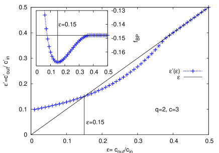
and . Starting with a suitable initial value , we compute and iterate until convergence (see Fig. 1), as in the expectation-maximization algorithm DempsterLaird77 . To learn the number of groups , we run the algorithm with several values of . The free energy decreases with and then stays constant for .
Phase diagrams.
For illustration we use the case of planted partitions and colorings, , for , and . We observe three different cases governing the free energy landscape . In the “paramagnetic” phase, the free energy is constant in the vicinity of the true value of . Learning is impossible, and the marginals are for all nodes. In this case the overlap between the original assignment and the one resulting from BP marginalization, defined as
| (4) |
(where is the permutation group) is zero, and the original assignment is undetectable. Generalizing AchlioptasCoja-Oghlan08-focs ; KrzakalaZdeborova09 , one can show there is essentially no difference between a graph produced by the block model and a completely random graph of the same average degree; the free energy of the two ensembles is asymptotically identical.
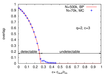
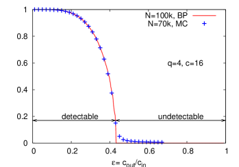
In the ordered phase, has an attractive global minimum at the true value of , and BP rapidly infers the correct parameters. This is illustrated in Fig. 2. As varies from ( completely separated groups) to (a pure random graph), we observe a continuous phase transition from an ordered phase with positive overlap to a paramagnetic phase with zero overlap. Thus there is a second-order transition from a detectable to an undetectable phase.
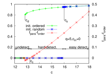
A third situation arises if has both a paramagnetic fixed point and the ordered fixed point at the true . In this case, the two phases co-exist and the detectability transition is first-order; see Fig. 2 on the right. The phase transition is located by comparing the free energies of the two phases. However, even if the ordered fixed point has a lower free energy, it is not easy to find it unless the initial messages are close to the true group assignment. All but an exponentially small set of initial messages will lead to the paramagnetic fixed point. This situation is typical of mean-field first-order phase transitions. In fact, recent results about random optimization problems show that finding the lower-free-energy phase in this case is an extremely hard problem FranzMezard01 ; KrzakalaZdeborova09 .
Only when the paramagnetic phase is no longer locally stable does inference become easy. We can compute the location of the transition to this easily-detectable phase analytically by analyzing how a small random perturbation to the paramagnetic fixed point propagates as the BP equations are iterated MezardMontanari06 ; KrzakalaZdeborova09 . It follows that for
| (5) |
the original group assignment is dynamically attractive and hence many algorithms, e.g. MC or BP, will converge to it. Note that it is typically still hard to compute the ground state of (2), even though we can compute the marginals, and therefore the optimal estimate of the group assignment, asymptotically exactly.
On the other hand, if (5) is not satisfied then community detection is either impossible, or at best as hard as solving the hardest known optimization problems. When the phase transition is of first-order for , as can be retrieved from data presented in MezardMontanari06 . However, the detectable but hard region is so narrow that is is quite unlikely to appear in realistic situations.
Real-world networks.
Our algorithm is not restricted to large random networks; it is applicable to real networks as well. We tested it on the “Karate Club” network Zachary77 , a common benchmark for community detection. For , BP leads to two different fixed points. One corresponds to the actual known division into two groups. The other has a smaller free energy and thus a larger likelihood, and splits the network into high-degree nodes and low-degree nodes as found in KarrerNewman10 . These two fixed points correspond to two local minima of for , and depending on the initial value BP converges to one or the other. For , our algorithm converges to fixed points with yet lower values of . For the best fixed point corresponds to a splitting of the two actual groups into high-degree and low-degree subgroups.
The results obtained with MC, which can be easily equilibrated for such a small network, are almost identical to those of BP in terms of the parameters and marginals, and identical in terms of the estimated group assignments. This demonstrates that BP is a useful approach even on real, finite networks that are far from trees.
Conclusion.
We have presented a principled and asymptotically exact analysis of the detection of communities in networks generated by the stochastic block model. There is a strict limit on detectability due to a transition from a phase where the free energy landscape lets us infer the model’s parameters, to a phase where it does not. In some cases the communities are detectable, but the problem is hard because the attractive region around the correct fixed point is exponentially small. Our analysis comes with an associated learning algorithm, which for large sparse networks generated from the model is able to learn the number of groups, their exact sizes, and the affinity matrix . Our approach and our algorithm are easily generalized to other local generative models, and we will investigate its performance on a variety of real-world networks in the future.
Acknowledgments.
We are grateful to Mark Newman for helpful discussions. C.M. is funded by the McDonnell Foundation.
References
- (1) S. Fortunato, Physics Reports 486, 75 (2010).
- (2) M. Mézard and G. Parisi, Eur. Phys. J. B 20, 217 (2001).
- (3) M. Mézard and A. Montanari, Physics, Information, Computation (Oxford Press, Oxford, 2009).
- (4) J. Reichardt and M. Leone, Phys. Rev. Lett. 101, 078701 (2008).
- (5) B. H. Good, Y.-A. de Montjoye, and A. Clauset, Phys. Rev. E 81, 046106 (2010).
- (6) J. Yedidia, W. Freeman, and Y. Weiss, Exploring Artificial Intelligence in the New Millennium (Morgan Kaufmann, San Francisco, CA, USA, 2003), pp. 239–236.
- (7) M. B. Hastings, Phys. Rev. E 74, 035102 (2006).
- (8) B. Karrer and M. E. J. Newman, (2010), arXiv:1008.3926.
- (9) M. E. J. Newman and M. Girvan, Phys. Rev. E 69, 026113 (2004).
- (10) J. M. Hofman and C. H. Wiggins, Phys. Rev. Lett. 100, 258701 (2008).
- (11) F. Krzakala and L. Zdeborová, Phys. Rev. Lett. 102, 238701 (2009).
- (12) M. E. J. Newman and E. A. Leicht, Proc. Natl. Acad. Sci. USA 104, 9564 (2007).
- (13) A. Clauset, C. Moore, and M. Newman, Nature 453, 98 (2008).
- (14) H. Nishimori, Statistical Physics of Spin Glasses and Information Processing: An Introduction (Oxford University Press, Oxford, UK, 2001).
- (15) D. Coppersmith, D. Gamarnik, M. T. Hajiaghayi, and G. B. Sorkin, Random Struct. Algorithms 24, 502 (2004).
- (16) A. Dempster, N. Laird, and D. Rubin, Journal of the Royal Statistical Society 39, 1–38 (1977).
- (17) D. Achlioptas and A. Coja-Oghlan, Proc. FOCS (2008).
- (18) S. Franz et al., Europhys. Lett. 55, 465 (2001).
- (19) M. Mézard and A. Montanari, J. Stat. Phys. 124, 1317 (2006).
- (20) W. W. Zachary, J. Anthropological Res. 33, 452 (1977).