Multi-Parameter Tikhonov Regularization

Abstract

We study multi-parameter Tikhonov regularization, i.e., with multiple penalties. Such models are useful when the sought-for solution exhibits several distinct features simultaneously. Two choice rules, i.e., discrepancy principle and balancing principle, are studied for choosing an appropriate (vector-valued) regularization parameter, and some theoretical results are presented. In particular, the consistency of the discrepancy principle as well as convergence rate are established, and an a posteriori error estimate for the balancing principle is established. Also two fixed point algorithms are proposed for computing the regularization parameter by the latter rule. Numerical results for several nonsmooth multi-parameter models are presented, which show clearly their superior performance over their single-parameter counterparts.
Key words: multi-parameter regularization, value function, balancing principle, parameter choice.

1 Introduction

In this paper, we are interested in solving linear inverse problems

$$Kx=y^{\delta},$$ (1)

where $y^{\delta}\in Y$ is a noisy version of the exact data $y^{\dagger}=Kx^{\dagger}\in Y$ with $\delta^{2}=\phi(x^{\dagger},y^{\delta})$ being the noise level, the operator $K:X\rightarrow Y$ is bounded and linear, and the spaces $X$ and $Y$ are Banach spaces.

Typically, problem (1) suffers from ill-posedness in the sense that a small perturbation in the data might lead to large deviations in the retrieved solution, and this often poses great challenges to their stable yet accurate numerical solution. Usually, a regularization strategy is applied to find a stable approximate solution [18, 6]. The most widely adopted approach is Tikhonov regularization, which seeks an approximation $x_{\boldsymbol{\eta}}^{\delta}$ to problem (1) by minimizing the following Tikhonov functional

$$J_{\boldsymbol{\eta}}(x)=\phi(x,y^{\delta})+\boldsymbol{\eta}\cdot\boldsymbol{\psi}(x).$$

Here the functionals $\phi$ and $\boldsymbol{\psi}$ represent data fidelity and (vector-valued) penalty, respectively, and $\boldsymbol{\eta}\cdot\boldsymbol{\psi}(x)$ is the dot product between $\boldsymbol{\eta}=(\eta_{1},\ldots,\eta_{n})^{\mathrm{T}}$ and $\boldsymbol{\psi}(x)=(\psi_{1}(x),\ldots,\psi_{n}(x))^{\mathrm{T}}$, i.e., $\boldsymbol{\eta}\cdot\boldsymbol{\psi}(x)=\sum_{i=1}^{n}\eta_{i}\psi_{i}(x)$. Common choices of the fidelity $\phi(x,y^{\delta})$ include $\|Kx-y^{\delta}\|_{L^{2}}^{2}$, $\|Kx-y^{\delta}\|_{L^{1}}$ and $\int(Kx-y^{\delta}\ln Kx)$, which are statistically well suited to additive Gaussian noise, Laplace (impulsive) noise and Poisson noise, respectively. The penalties $\psi_{i}$ are nonnegative, convex and (weak) lower semicontinuous. The typical choice includes $\|x\|_{L^{2}}^{2}$, $\|x\|_{\ell^{p}}^{p}$, $\|x\|_{H^{m}}^{2}$ and $|x|_{TV}$ etc. The regularization parameter vector $\boldsymbol{\eta}$ compromises fidelity with penalties.

The use of multiple penalties, henceforth called multi-parameter regularization, in the functional $J_{\boldsymbol{\eta}}$ is motivated by practical applications which exhibit multiple/multiscale features. We just take microarray data analysis for an example. Here the number of data is often far less than that of the unknowns. A desirable approach should select all variables relevant to the proper functioning of gene network. The conventional $\ell^{2}$ penalty tends to select all variables, including irrelevant ones, since the resulting estimate has almost no nonzero entries. To remedy this issue, $\ell^{1}$ penalty has been suggested as an alternative. However, the $\ell^{1}$ approach delivers undesirable results for problems where there are highly correlated features and all relevant ones are to be identified in that it tends to select only one feature out of the relevant group instead of all relevant features of the group [20], thereby missing the groupwise structure. Zou and Hastie [20] proposed the elastic-net by incorporating the $\ell^{2}$ penalty into the $\ell^{1}$ penalty, in the hope of retrieving the whole relevant group, and numerically demonstrated its excellent performance for simulation studies and real-data applications. Such multiple/multiscale features appear also in many other applications, e.g., image processing [14, 17], electrocardiography [3], and geodesy [19].

A number of experimental studies [3, 20, 19] have shown great potential of multi-parameter models for better capturing multiple distinct features of the solution. However, a general theory for such models remains largely under-explored. There are several attempts on various aspects, e.g., parameter choice, convergence and statistical interpretation [1, 2, 4, 9, 5, 12, 13] of multi-parameter regularization. For instance, Lu et al [12] discussed the discrepancy principle using Hilbert space scales, and derived some error estimates, but the parameter is vastly nonunique and it remains unclear which one to use. They also adapted the model function approach to choose the regularization parameter, but the underlying mechanism remains unclear. Jin et al [9] recently investigated the properties, e.g., consistency and error estimates, of elastic-net for asymptotically linear coupling between the two terms, and proposed two active-set type methods for efficient numerical realization.

This paper aims at developing some theory for such models in a general framework. The value function and its properties are first derived. Then two parameter choice rules, i.e., discrepancy principle and balancing principle, are studied. The consistency and convergence rates are established for the former. The balancing principle can be derived from the Bayesian inference [10], and it was generalized in [8]. The principle balances the penalty with the fidelity term. The variant under consideration here is solely based on the value function, and does not require a knowledge of the noise level. An a posteriori error estimate is derived, and two efficient numerical algorithms are also proposed.

The rest of the paper is structured as follows. In Section 2, we investigate the value function and derive some properties, e.g., monotonicity, concavity, asymptotic and especially differentiability. In Section 3, we investigate two parameter choice rules, i.e., discrepancy principle and balancing principle, and discuss their theoretical properties. In addition, two fixed point algorithms for the efficient numerical realization of the balancing principle are proposed. Numerical results for several examples are presented in Section 4 to illustrate the efficiency and accuracy of the proposed approaches. Finally, we conclude the paper with several future research topics.

Notation

Let $x_{\boldsymbol{\eta}}^{\delta}$ be a minimizer to the functional $J_{\boldsymbol{\eta}}(x)$, and $\mathcal{M}_{\boldsymbol{\eta}}$ be the set of minimizers. For vectors $\boldsymbol{\eta}\in\mathbb{R}^{n}$ and $\hat{\boldsymbol{\eta}}\in\mathbb{R}^{n}$, we denote by ${\boldsymbol{\eta}}\leq\hat{\boldsymbol{\eta}}$ if $\eta_{i}\leq\hat{\eta}_{i}\,\forall 1\leq i\leq n$.

2 The value function and its properties

In this section, we collect important properties of the value function $F(\boldsymbol{\eta})$ defined by

$$F(\boldsymbol{\eta})=\inf_{x\in Q_{\text{ad}}}J_{\boldsymbol{\eta}}(x),$$ (2)

where the set $Q_{\mathrm{ad}}$ stands for a convex constraint. Here, the existence of a minimizer $x_{\boldsymbol{\eta}}^{\delta}$ to the functional $J_{\boldsymbol{\eta}}$ is not a priori assumed. Provided that a minimizer $x_{\boldsymbol{\eta}}^{\delta}$ does exist, we have $F(\boldsymbol{\eta})=J_{\boldsymbol{\eta}}(x_{\boldsymbol{\eta}}^{\delta})$. The value function $F$ will play an important role in developing a balancing principle, see Section 3.2. The results presented below generalize those for the single parameter [7], and the proofs are similar and thus omitted.

A first result shows the continuity and concavity of $F$.

Lemma 2.1.

The value function $F(\boldsymbol{\eta})$ is monotonically increasing in the sense $F(\hat{\boldsymbol{\eta}})\leq F(\boldsymbol{\eta})$ if $\hat{\boldsymbol{\eta}}\leq\boldsymbol{\eta}$, and it is concave.

Remark 2.1.

Lemma 2.1 does not require the existence of $x\in Q_{\mathrm{ad}}$ that achieves the infimum of $J_{\boldsymbol{\eta}}$. The results are also true for nonlinear operators and in the presence of convex constraint $Q_{\mathrm{ad}}$.

Next we examine the properties of the value function $F$ more closely. Recall first one-sided partial derivatives $\partial^{\pm}_{i}F$ are defined by

$$\partial^{-}_{i}F(\boldsymbol{\eta})=\lim_{h\rightarrow 0^{+}}\frac{F({\boldsymbol{\eta}})-F({\boldsymbol{\eta}}-h\boldsymbol{e}_{i})}{h},$$

$$\partial^{+}_{i}F({\boldsymbol{\eta}})=\lim_{h\rightarrow 0^{+}}\frac{F({\boldsymbol{\eta}}+h\boldsymbol{e}_{i})-F({\boldsymbol{\eta}})}{h},$$

where $\boldsymbol{e}_{i}$ is the $i$th canonical basis.

The next result shows some properties, i.e., existence, nonnegativity, monotonicity and (left- and right-) continuity, of the one-side partial derivatives $\partial_{i}^{\pm}F$. The properties follow directly from Lemma 2.1.

Lemma 2.2.

For any $\boldsymbol{\eta}>0$, there hold

• The one-sided partial derivatives $\partial_{i}^{\pm}F(\boldsymbol{\eta})$ exist, and $\partial_{i}^{\pm}F(\boldsymbol{\eta})\geq 0$;

• For any $h>0$, there holds $0\leq\partial_{i}^{+}F(\boldsymbol{\eta}+h\boldsymbol{e}_{i})\leq\partial_{i}^{-}F(\boldsymbol{\eta}+h\boldsymbol{e}_{i})\leq\partial_{i}^{+}F(\boldsymbol{\eta})\leq\partial_{i}^{-}F(\boldsymbol{\eta})$;

• $\displaystyle\partial_{i}^{-}F(\boldsymbol{\eta})=\lim_{h\rightarrow 0^{+}}\partial_{i}^{-}F(\boldsymbol{\eta}-h\boldsymbol{e}_{i})$ and $\displaystyle\partial_{i}^{+}F(\boldsymbol{\eta})=\lim_{h\rightarrow 0^{+}}\partial_{i}^{+}F(\boldsymbol{\eta}+h\boldsymbol{e}_{i})$.

Remark 2.2.

The partial differentiability of $F$ in the $i$-th direction at ${\boldsymbol{\eta}}$ guarantees the continuity of $\partial_{i}^{\pm}F$ at this point. Indeed, the monotonicity of $\partial_{i}^{\pm}F$ and the left continuity of $\partial_{i}^{+}F$ yield the inequalities

$$\partial_{i}^{+}F({\boldsymbol{\eta}})=\lim_{h\rightarrow 0^{+}}\partial_{i}^{+}F({\boldsymbol{\eta}}+h\boldsymbol{e}_{i})\leq\lim_{h\rightarrow 0^{+}}\partial_{i}^{-}F({\boldsymbol{\eta}}+h\boldsymbol{e}_{i})\leq\partial_{i}^{-}F({\boldsymbol{\eta}}).$$

Now suppose $F$ is differentiable at ${\boldsymbol{\eta}}$, i.e., $\partial_{i}^{-}F({\boldsymbol{\eta}})=\partial_{i}^{+}F({\boldsymbol{\eta}})$. Then from the inequalities it follows that

$$\lim_{h\rightarrow 0^{+}}\partial_{i}^{-}F({\boldsymbol{\eta}}+h\boldsymbol{e}_{i})=\partial_{i}^{-}F({\boldsymbol{\eta}}),$$

which shows the continuity of $\partial_{i}^{-}F$ at ${\boldsymbol{\eta}}$. Similarly it follows that $\partial_{i}^{+}F$ is continuous at ${\boldsymbol{\eta}}$.

The asymptotic behavior of $F(\boldsymbol{\eta})$ is useful for designing numerical algorithms.

Proposition 2.1.

The following asymptotics of $F$ hold

$$\lim_{|\boldsymbol{\eta}|\rightarrow 0}F(\boldsymbol{\eta})=\inf_{x\in Q_{\text{ad}}}\phi(x,y^{\delta})\quad\mbox{and}\quad\lim_{|\boldsymbol{\eta}|\rightarrow 0}\eta_{i}\partial_{i}^{\pm}F(\boldsymbol{\eta})=0.$$

The partial derivatives $\partial_{i}^{\pm}F$ are closely connected to the fidelity $\phi$ and penalty $\boldsymbol{\psi}$ under the assumption of existence of a minimizer, i.e., the set $\mathcal{M}_{\boldsymbol{\eta}}$ is nonempty. This is guaranteed by:

Assumption 2.1.

The functionals $\phi$ and $\psi_{i}$ satisfy:

• For any sequence $\{x_{n}\}_{n}\subset Q_{\mathrm{ad}}$ such that $\phi$ and $\psi_{i}$ for all $1\leq i\leq n$ are uniformly bounded, there exists a subsequence $\{x_{n_{k}}\}_{k}$ which converges to an element $x^{*}\in Q_{ad}$ in the $\tau$-topology.

• $\phi$ and $\psi_{i}$ are lower semi-continuous with respect to $\tau$-convergent sequences, i.e., if a subsequence $\{x_{n}\}_{n}$ converges to $x^{*}\in Q_{\mathrm{ad}}$ in $\tau$-topology, then

  $$\phi(x^{*})\leq\liminf_{n\to\infty}\phi(x_{n})\mbox{ and }\,\psi_{i}(x^{*})\leq\liminf_{n\to\infty}\psi_{i}(x_{n}).$$

In case that the set $\mathcal{M}_{\boldsymbol{\eta}}$ contains multiple elements, there might exist distinct $x_{\boldsymbol{\eta}}^{\delta},\hat{x}_{\boldsymbol{\eta}}^{\delta}\in\mathcal{M}_{\eta}$ such that

$$F(\eta)=\phi(x_{\boldsymbol{\eta}}^{\delta},y^{\delta})+\boldsymbol{\eta}\cdot\boldsymbol{\psi}(x_{\boldsymbol{\eta}}^{\delta})=\phi(\hat{x}_{\boldsymbol{\eta}}^{\delta},y^{\delta})+\boldsymbol{\eta}\cdot\boldsymbol{\psi}(\hat{x}_{\boldsymbol{\eta}}^{\delta})\quad\mbox{but}\quad\phi(x_{\boldsymbol{\eta}}^{\delta},y^{\delta})\neq\phi(\hat{x}_{\boldsymbol{\eta}}^{\delta},y^{\delta}),$$

i.e., the functions $\phi(x_{\boldsymbol{\eta}}^{\delta},y^{\delta})$ and $\boldsymbol{\psi}(x_{\boldsymbol{\eta}}^{\delta})$ are potentially multi-valued in $\boldsymbol{\eta}$.

A first relation between $\psi_{i}$ and $\partial_{i}^{\pm}F$ is given by

Lemma 2.3.

Let Assumption 2.1 be fulfilled. Then for any $x_{\boldsymbol{\eta}}^{\delta}\in\mathcal{M}_{\boldsymbol{\eta}}$, there hold

$$\partial_{i}^{+}F({\boldsymbol{\eta}})\leq\ \psi_{i}(x_{\boldsymbol{\eta}}^{\delta})\leq\partial_{i}^{-}F({\boldsymbol{\eta}})\quad i=1,\ldots,n,$$

$$F({\boldsymbol{\eta}})-\sum_{i=1}^{n}\eta_{i}\partial_{i}^{-}F(\boldsymbol{\eta})\leq\ \phi(x_{\boldsymbol{\eta}}^{\delta},y^{\delta})\leq F(\boldsymbol{\eta})-\sum_{i=1}^{n}\eta_{i}\partial_{i}^{+}F(\boldsymbol{\eta}).$$

An immediate consequence of Lemma 2.3 is:

Corollary 2.1.

Let Assumption 2.1 be fulfilled. If $\partial_{i}F(\boldsymbol{\eta})$ exists $\boldsymbol{\eta}$ for all $i$, then $\psi_{i}(x_{\boldsymbol{\eta}}^{\delta})$ and $\phi(x_{\boldsymbol{\eta}}^{\delta},y^{\delta})$ are single valued at $\boldsymbol{\eta}$ and

$$\partial_{i}F(\boldsymbol{\eta})=\psi_{i}(x_{\boldsymbol{\eta}}^{\delta})\quad\mbox{and}\quad F(\boldsymbol{\eta})-\boldsymbol{\eta}\cdot\partial F(\boldsymbol{\eta})=\phi(x_{\boldsymbol{\eta}}^{\delta},y^{\delta})\quad\forall x_{\boldsymbol{\eta}}^{\delta}\in\mathcal{M}_{\boldsymbol{\eta}}.$$

More precisely, the partial derivatives $\partial^{\pm}_{i}$ can be expressed by $\psi_{i}$ as follows.

Theorem 2.1.

Let Assumption 2.1 hold. Then for any $\boldsymbol{\eta}>0$ and every $i$, there exist $x^{+}_{i},x^{-}_{i}\in\mathcal{M}_{\boldsymbol{\eta}}$ such that

$$\psi_{i}(x^{+}_{i})=\partial_{i}^{+}F(\boldsymbol{\eta})\quad\mbox{and}\quad\psi_{i}(x^{-}_{i})=\partial_{i}^{-}F(\boldsymbol{\eta}).$$

Theorem 2.1 in conjunction with Lemma 2.3 implies the following corollary.

Corollary 2.2.

Let Assumption 2.1 hold. Then

• There exist $x^{+}_{i},x^{-}_{i}\in\mathcal{M}_{\boldsymbol{\eta}}$ such that $\displaystyle\psi_{i}(x^{+}_{i})=\min_{x\in\mathcal{M}_{\boldsymbol{\eta}}}\psi_{i}(x)$ and $\displaystyle\psi_{i}(x^{-}_{i})=\max_{x\in\mathcal{M}_{\boldsymbol{\eta}}}\psi_{i}(x)$.

• If $\psi_{i}(x_{\boldsymbol{\eta}}^{\delta})=\psi_{i}(\hat{x}_{\boldsymbol{\eta}}^{\delta})$ for all $x_{\boldsymbol{\eta}}^{\delta},\hat{x}_{\boldsymbol{\eta}}^{\delta}\in\mathcal{M}_{\boldsymbol{\eta}}$ for all ${\boldsymbol{\eta}}>0$, then $\partial_{i}F({\boldsymbol{\eta}})$ exists and it is continuous.

The last result gives a sufficient condition for the differentiability of the value function $F$. It plays an important role in especially designing an efficient algorithm for certain choice rules, by e.g., Morozov’s principle and balancing principle [11].

Theorem 2.2.

Assume that the minimizer of the functional $J_{\boldsymbol{\eta}}$ is unique at ${\boldsymbol{\eta}}>0$. Then the derivatives $\{\partial_{i}F({\boldsymbol{\eta}})\}_{i}$ exist and are continuous at $\boldsymbol{\eta}$. In particular, $F$ is differentiable at ${\boldsymbol{\eta}}$.

3 Parameter choice rules

In this section, we discuss two choice rules, i.e., discrepancy principle [16, 10] and balancing principle [7], for multi-parameter models. For notational simplicity, we shall restrict our attention to the case of two penalty terms.

3.1 Discrepancy principle

Here we investigate the discrepancy principle due to Morozov [16] for multi-parameter regularization. We shall assume a triangle-type inequality for the functional $\phi$.

Assumption 3.1.

The functional $\phi(x,y)$ vanishes if and only if $Kx=y$, and satisfies an inequality $\phi(x,y)\leq c(\phi(x^{\prime},y^{\prime})+\phi(x,y^{\prime}))$ for some constant $c$ and any $x^{\prime}$ with $Kx^{\prime}=y$.

The discrepancy principle determines an appropriate (vector-valued) regularization parameter $\boldsymbol{\eta}$ by

$$\phi(x_{\boldsymbol{\eta}}^{\delta},y^{\delta})=c_{m}\delta^{2}$$ (3)

for some constant $c_{m}\geq 1$. The rationale of the principle is that the solution accuracy in terms of the residual should be compatible with the data accuracy (noise level).

Theorem 3.1.

Let Assumptions 2.1 and 3.1 be satisfied and the operator $K$ be injective. Then for any $\boldsymbol{\eta}\equiv\boldsymbol{\eta}(\delta)$ satisfying (3) and $c_{0}\leq\tfrac{\eta_{1}(\delta)}{\eta_{2}(\delta)}\leq c_{1}$ for some $c_{0},c_{1}>0$, there holds $\lim_{\delta\rightarrow 0}x_{\boldsymbol{\eta}}^{\delta}=x^{\dagger}$ in $\tau$-topology.

Proof.

The minimizing property of $x_{\boldsymbol{\eta}}^{\delta}$ implies

$$\phi(x_{\boldsymbol{\eta}}^{\delta},y^{\delta})+\boldsymbol{\eta}\cdot\boldsymbol{\psi}(x_{\boldsymbol{\eta}}^{\delta}) \leq\phi(x^{\dagger},y^{\delta})+\boldsymbol{\eta}\cdot\boldsymbol{\psi}(x^{\dagger})$$

$$\leq\delta^{2}+\boldsymbol{\eta}\cdot\boldsymbol{\psi}(x^{\dagger}).$$

From the discrepancy equation (3), we deduce

$$\boldsymbol{\eta}\cdot\boldsymbol{\psi}(x_{\boldsymbol{\eta}}^{\delta})\leq\boldsymbol{\eta}\cdot\boldsymbol{\psi}(x^{\dagger}).$$ (4)

Therefore, either $\psi_{1}(x_{\boldsymbol{\eta}}^{\delta})\leq\psi_{1}(x^{\dagger})$ or $\psi_{2}(x_{\boldsymbol{\eta}}^{\delta})\leq\psi_{2}(x^{\dagger})$ holds. Now the assumption $c_{0}\leq\frac{\eta_{1}(\delta)}{\eta_{2}(\delta)}\leq c_{1}$ implies that the sequence $\{\psi_{i}(x_{\boldsymbol{\eta}}^{\delta}),i=1,2\}_{\delta}$ is uniformly bounded. Hence the coercivity of the functional indicates that the sequence $\{x_{\boldsymbol{\eta}}^{\delta}\}_{\delta}$ is uniformly bounded. Thus there exists a subsequence, also denoted by $\{x_{\boldsymbol{\eta}}^{\delta}\}_{\delta}$, and some $x^{\ast}$, such that

$$x_{\boldsymbol{\eta}}^{\delta}\rightarrow x^{\ast}\quad\mbox{ in $\tau$-topology}.$$

The $\tau$-lower semicontinuity of the functional $\phi$ and Assumption 3.1 yields

$$0\leq\phi(x^{\ast},y^{\dagger})\leq c\liminf_{\delta\rightarrow 0}(\phi(x^{\dagger},y^{\delta})+\phi(x_{\boldsymbol{\eta}}^{\delta},y^{\delta}))\leq\liminf_{\delta\rightarrow 0}c(1+c_{m})\delta^{2}=0.$$

In particular, $\phi(x^{\ast},y^{\dagger})=0$, i.e., $Kx^{\ast}=y^{\dagger}$. This together with the injectivity $K$ implies $x^{\ast}=x^{\dagger}$. Since every subsequence has a subsubsequence converging to $x^{\dagger}$, the whole sequence converges to $x^{\dagger}$. ∎

Remark 3.1.

The condition $c_{0}\leq\tfrac{\eta_{1}(\delta)}{\eta_{2}(\delta)}\leq c_{1}$ ensures the uniform boundedness of both penalties, and thus we can utilize the lower-semicontinuity of the functionals to arrive at the desired $\tau$-convergence.

Theorem 3.2.

Let Assumptions 2.1 and 3.1 hold. If a subsequence $\{\boldsymbol{\eta}(\delta)\}_{\delta}$ converges and $\displaystyle\tilde{\eta}\equiv\lim_{\delta\rightarrow 0}\tfrac{\eta_{1}(\delta)}{\eta_{2}(\delta)}>0$. Then it contains a subsequence $\tau$-converging to an $\tilde{\eta}\psi_{1}+\psi_{2}$-minimizing solution and

$$\lim_{\delta\rightarrow 0}\left(\frac{\eta_{1}(\delta)}{\eta_{2}(\delta)}\psi_{1}(x_{\boldsymbol{\eta}}^{\delta})+\psi_{2}(x_{\boldsymbol{\eta}}^{\delta})\right)=\tilde{\eta}\psi_{1}(x^{\dagger})+\psi_{2}(x^{\dagger}).$$

Moreover, if the $\tilde{\eta}\psi_{1}+\psi_{2}$-minimizing solution is unique, then the whole subsequence $\tau$-converges.

Proof.

By repeating the arguments in Theorem 3.1, we deduce that there exists a subsequence, also denoted by $\{x_{\boldsymbol{\eta}}^{\delta}\}_{\delta}$, and some $x^{\ast}$, such that

$$x_{\boldsymbol{\eta}}^{\delta}\rightarrow x^{\ast}\quad\mbox{ in $\tau$-topology}.$$

and by the $\tau$-lower-semicontinuity, we have $\phi(x^{\ast},y^{\dagger})=0$. By virtue of lower semicontinuity of the functionals and inequality (4), we deduce

$$\tilde{\eta}\psi_{1}(x^{\ast})+\psi_{2}(x^{\ast}) \leq\liminf_{\delta\rightarrow 0}\left(\frac{\eta_{1}(\delta)}{\eta_{2}(\delta)}\psi_{1}(x_{\boldsymbol{\eta}}^{\delta})+\psi_{2}(x_{\boldsymbol{\eta}}^{\delta})\right)$$

$$\leq\limsup_{\delta\rightarrow 0}\left(\frac{\eta_{1}(\delta)}{\eta_{2}(\delta)}\psi_{1}(x_{\boldsymbol{\eta}}^{\delta})+\psi_{2}(x_{\boldsymbol{\eta}}^{\delta})\right)$$

$$\leq\lim_{\delta\rightarrow 0}\left(\frac{\eta_{1}(\delta)}{\eta_{2}(\delta)}\psi_{1}(x^{\dagger})+\psi_{2}(x^{\dagger})\right)=\tilde{\eta}\psi_{1}(x^{\dagger})+\psi_{2}(x^{\dagger}),$$

which together with the identity $\phi(x^{\ast},y^{\dagger})=0$ implies that $x^{\ast}$ is an $\tilde{\eta}\psi_{1}+\psi_{2}$-minimizing solution. The desired identity follows from the above inequalities with $x^{\ast}$ in place of $x^{\dagger}$. The whole sequence convergence follows from the standard subsequence argument. ∎

In Theorems 3.1 and 3.2, we have assumed the existence of a solution $\boldsymbol{\eta}$ to equation (3). This is guaranteed if the Tikhonov functional $J_{\boldsymbol{\eta}}$ has a unique minimizer, see Theorem 2.2.

Theorem 3.3.

Assume that $J_{\boldsymbol{\eta}}$ has a unique minimizer for all $\boldsymbol{\eta}>0$, $\lim_{|\boldsymbol{\eta}|\rightarrow 0}\phi(x_{\boldsymbol{\eta}}^{\delta},y^{\delta})<c_{m}\delta^{2}$, and there is a sequence $\{\boldsymbol{\eta}_{n}\}$ such that $\lim_{n\rightarrow\infty}\phi(x_{\boldsymbol{\eta}_{n}}^{\delta},y^{\delta})>c_{m}\delta^{2}$. Then there exists at least one solution to (3).

Proof.

By Theorem 2.2 and Lemma 2.1, the uniqueness of a minimizer to $J_{\boldsymbol{\eta}}$ for all $\boldsymbol{\eta}>0$ implies that the function $\phi(x_{\boldsymbol{\eta}}^{\delta},y^{\delta})$ is continuous in $\boldsymbol{\eta}$. The desired assertion follows from the continuity directly. ∎

Lastly, we present an error estimate in case of $Y$ being a Hilbert space and $\phi(x,y^{\delta})=\|Kx-y^{\delta}\|^{2}$ and convex penalties $\boldsymbol{\psi}$. We use Bregman distance to measure the error. Denote the subdifferential of a functional $\psi(x)$ at $x^{\dagger}$ by $\partial\psi(x^{\dagger})$, i.e., $\partial\psi(x^{\dagger})=\{\xi\in X^{\ast}:\psi(x)\geq\psi(x^{\dagger})+\langle\xi,x-x^{\dagger}\rangle\,\forall x\in X\}$, and the Bregman distance $d_{\xi}(x,x^{\dagger})$ by for any $\xi\in\partial\psi(x^{\dagger})$

$$d_{\xi}(x,x^{\dagger}):=\psi(x)-\psi(x^{\dagger})-\langle\xi,x-x^{\dagger}\rangle.$$

Theorem 3.4.

If $Y$ is a Hilbert space and the exact solution $x^{\dagger}$ satisfies the source condition: $\mathrm{range}(K^{\ast})\cap\partial\psi_{1}(x^{\dagger})\cap\partial\psi_{2}(x^{\dagger})\neq\emptyset$. Then for any $\boldsymbol{\eta}^{\ast}$ solving (3), there exists some $i$ and $\xi_{i}\in\partial\psi_{i}(x^{\dagger})$ such that

$$d_{\xi_{i}}(x_{\boldsymbol{\eta}^{\ast}}^{\delta},x^{\dagger})\leq C\delta.$$

Proof.

By the minimizing property of $x_{\boldsymbol{\eta}^{\ast}}^{\delta}$, we have

$$\phi(x_{\boldsymbol{\eta}^{\ast}}^{\delta},y^{\delta})+\boldsymbol{\eta}^{\ast}\cdot\boldsymbol{\psi}(x_{\boldsymbol{\eta}^{\ast}}^{\delta})\leq\phi(x^{\dagger},y^{\delta})+\boldsymbol{\eta}^{\ast}\cdot\boldsymbol{\psi}(x^{\dagger})\leq\delta^{2}+\boldsymbol{\eta}^{\ast}\cdot\boldsymbol{\psi}(x^{\dagger}).$$

The definition of the discrepancy principle indicates

$$\boldsymbol{\eta}^{\ast}\cdot\boldsymbol{\psi}(x_{\boldsymbol{\eta}^{\ast}}^{\delta})\leq\boldsymbol{\eta}^{\ast}\cdot\boldsymbol{\psi}(x^{\dagger}).$$

Consequently, we have that there holds $\psi_{i}(x_{\boldsymbol{\eta}^{\ast}}^{\delta})\leq\psi_{i}(x^{\dagger})$ for either $i=1$ or $i=2$. Therefore, by the source condition, for some $\xi_{i}\in\mathrm{range}(K^{\ast})\cap\partial\psi_{i}(x^{\dagger})$ or equivalently $\xi_{i}=K^{\ast}w_{i}$ for some source representer $w_{i}$, and the Cauchy-Schwarz inequality, we deduce

$$d_{\xi_{i}}(x_{\boldsymbol{\eta}^{\ast}}^{\delta},x^{\dagger}) =\psi_{i}(x_{\boldsymbol{\eta}^{\ast}}^{\delta})-\psi_{i}(x^{\dagger})-\langle\xi_{i},x_{\boldsymbol{\eta}^{\ast}}^{\delta}-x^{\dagger}\rangle\leq-\langle\xi_{i},x_{\boldsymbol{\eta}^{\ast}}^{\delta}-x^{\dagger}\rangle$$

$$=-\langle K^{\ast}w_{i},x_{\boldsymbol{\eta}^{\ast}}^{\delta}-x^{\dagger}\rangle=-\langle w_{i},K(x_{\boldsymbol{\eta}^{\ast}}^{\delta}-x^{\dagger})\rangle$$

$$\leq\|w_{i}\|\|K(x_{\boldsymbol{\eta}^{\ast}}^{\delta}-x^{\dagger})\|$$

$$\leq\|w_{i}\|\left(\|Kx_{\boldsymbol{\eta}^{\ast}}^{\delta}-y^{\delta}\|+\|y^{\delta}-Kx^{\dagger}\|\right)\leq(1+c_{m})\|w_{i}\|\delta.$$

This shows the desired estimate. ∎

The source condition in Theorem 3.4 can be hard to argue. Alternatively, we can have another convergence rates result under a seemingly less restrictive assumption.

Theorem 3.5.

If $Y$ is a Hilbert space and the exact solution $x^{\dagger}$ satisfies the source condition: for any $t\in[0,1]$, there exists $w_{t}$ such that $K^{\ast}w_{t}=\xi_{t}\in\partial(t\psi_{1}(x^{\dagger})+(1-t)\psi_{2}(x^{\dagger}))$. Then for any $\boldsymbol{\eta}^{\ast}$ solving (3), and letting $t^{*}=\tfrac{\eta_{1}^{\ast}(\delta)}{\eta_{1}^{\ast}(\delta)+\eta_{2}^{\ast}(\delta)}$, the following estimate holds

$$d_{\xi_{t^{*}}}(x_{\boldsymbol{\eta}^{\ast}}^{\delta},x^{\dagger})\leq C\delta.$$

Proof.

By the minimizing property of $x_{\boldsymbol{\eta}^{\ast}}^{\delta}$, we have

$$t^{*}\psi_{1}(x_{\boldsymbol{\eta}^{\ast}}^{\delta})+(1-t^{*})\psi_{2}(x_{\boldsymbol{\eta}^{\ast}}^{\delta})\leq t^{*}\psi_{1}(x^{\dagger})+(1-t^{*})\psi_{2}(x^{\dagger}).$$

Therefore, by the source condition, for some $\xi_{t^{*}}\in\partial(t^{*}\psi(x^{\dagger})+(1-t^{*})\psi(x^{\dagger}))$ and $w_{t^{*}}\in Y$ such that $\xi_{t^{*}}=K^{\ast}w_{t^{*}}$, and the Cauchy-Schwarz inequality, we deduce

$$d_{\xi_{t^{*}}}(x_{\boldsymbol{\eta}^{\ast}}^{\delta},x^{\dagger}) =(t^{\ast}\psi_{1}(x_{\boldsymbol{\eta}^{\ast}}^{\delta})+(1-t^{\ast})\psi_{2}(x_{\boldsymbol{\eta}^{\ast}}^{\delta}))-(t^{\ast}\psi_{1}(x^{\dagger})+(1-t^{\ast})\psi_{2}(x^{\dagger}))-\langle\xi_{t^{*}},x_{\boldsymbol{\eta}^{\ast}}^{\delta}-x^{\dagger}\rangle$$

$$\leq-\langle\xi_{t^{*}},x_{\boldsymbol{\eta}^{\ast}}^{\delta}-x^{\dagger}\rangle=-\langle K^{\ast}w_{t^{*}},x_{\boldsymbol{\eta}^{\ast}}^{\delta}-x^{\dagger}\rangle$$

$$=-\langle w_{t^{*}},K(x_{\boldsymbol{\eta}^{\ast}}^{\delta}-x^{\dagger})\rangle\leq\|w_{t^{*}}\|\|K(x_{\boldsymbol{\eta}^{\ast}}^{\delta}-x^{\dagger})\|$$

$$\leq\|w_{t^{*}}\|\left(\|Kx_{\boldsymbol{\eta}^{\ast}}^{\delta}-y^{\delta}\|+\|y^{\delta}-Kx^{\dagger}\|\right)\leq(1+c_{m})\|w_{t^{*}}\|\delta.$$

This shows the desired estimate. ∎

Remark 3.2.

In the practical applications of the discrepancy principle, one needs to find the solution of a nonlinear equation in $\boldsymbol{\eta}$. The uniqueness of a solution to equation (3) is not guaranteed, and additional conditions need to be supplied for definiteness. Lastly, we would like to mention that the principle can be efficiently realized by the model function approach [11].

3.2 Balancing principle

The discrepancy principle described earlier requires an estimate of the noise level $\delta$, which is not always available in practical applications. Therefore, it is of great interest to develop heuristic rules that do not require this knowledge. One such rule is the balancing principle, for which there are several variants, see [8] for details. The principle can be derived from the augmented Tikhonov (a-Tikhonov) regularization [10], which admits clear statistical interpretations as hierarchical Bayesian modeling. In particular, it provides the mechanism to automatically balance the penalty with the fidelity, see also Remark 3.4. The variant under consideration is due to [7], and has demonstrate very promising empirical results for several common single-parameter models [7]. Finally we remind the balancing principle discussed here should not be confused with the principle due to Lepskii which is sometimes also named balancing principle [15] and does require a precise knowledge of the noise level.

First we first sketch the a-Tikhonov regularization approach. For multi-parameter models, it can be derived analogously from Bayesian inference [10, 8], and the resulting a-Tikhonov functional $J(x,\tau,\{\lambda_{i}\})$ is given by

$$J(x,\tau,\{\lambda_{i}\})=\tau\phi(x,y^{\delta})+\boldsymbol{\lambda}\cdot\boldsymbol{\psi}(x)+\sum_{i}(\beta_{i}\lambda_{i}-\alpha_{i}\ln\lambda_{i})+\beta_{0}\tau-\alpha_{0}\ln\tau,$$

which maximizes the posteriori probability density function $p(x,\tau,\{\lambda_{i}\}|y^{\delta})\propto\,p(y^{\delta}|x,\tau,\{\lambda_{i}\})\ p(x,\tau,\{\lambda_{i}\})$ under the assumption that the scalars $\{\lambda_{i}\}$ and $\tau$ have the Gamma distribution with known parameter pairs $(\alpha_{i},\beta_{i})$ and $(\alpha_{0},\beta_{0})$, respectively. Let $\eta_{i}=\frac{\lambda_{i}}{\tau}$. Then the necessary optimality condition of the a-Tikhonov functional is given by

$$\left\{\begin{aligned} x^{\delta}_{\boldsymbol{\eta}}&=\arg\min_{x}\;\left\{\phi(x,y^{\delta})+\boldsymbol{\eta}\cdot\boldsymbol{\psi}(x)\right\},\\ \lambda_{i}&=\dfrac{\alpha_{i}}{\psi_{i}(x^{\delta}_{\boldsymbol{\eta}})+\beta_{i}},\\ \tau&=\dfrac{\alpha_{0}}{\phi(x_{\boldsymbol{\eta}}^{\delta},y^{\delta})+\beta_{0}}.\end{aligned}\right.$$

Upon assuming $\alpha_{i}=\alpha$ and $\beta_{i}=\beta$ for simplicity and letting $\gamma=\frac{\alpha_{0}}{\alpha}$, then we have the following system for $(x^{\delta}_{\boldsymbol{\eta}},{\boldsymbol{\eta}})$

$$\left\{\begin{aligned} x^{\delta}_{\boldsymbol{\eta}}&=\arg\min_{x}\;\left\{\phi(x,y^{\delta})+{\boldsymbol{\eta}}\cdot{\boldsymbol{\psi}}(x)\right\},\\ \eta_{i}&=\frac{1}{\gamma}\,\dfrac{\phi(x^{\delta}_{\boldsymbol{\eta}},y^{\delta})+\beta_{0}}{\psi_{i}(x^{\delta}_{\boldsymbol{\eta}})+\beta}.\end{aligned}\right.$$ (5)

Next, we give the promised balancing principle. The multi-parameter counterpart of the balancing principle given in [7] consists of minimizing

$$\Phi_{\gamma}({\boldsymbol{\eta}})=c_{\gamma}\frac{F^{2+\gamma}(\boldsymbol{\eta})}{\eta_{1}\eta_{2}},$$

where the constant $c_{\gamma}=\frac{\gamma^{\gamma}}{(\gamma+2)^{\gamma+2}}$. We note that this constant $c_{\gamma}$ can be quite arbitrary, except for comparison with the criterion $\Psi_{\gamma}$ defined next. Another variant of the balancing principle reads

$$\Psi_{\gamma}({\boldsymbol{\eta}})=\phi(x_{\boldsymbol{\eta}}^{\delta},y^{\delta})^{\gamma}\psi_{1}(x_{\boldsymbol{\eta}}^{\delta})\psi_{2}(x_{\boldsymbol{\eta}}^{\delta}),$$

which generalizes a criterion due to Reginska [6].

The relation between $\Phi_{\gamma}$ and $\Psi_{\gamma}$ is made explicit in the following result.

Proposition 3.1.

Let the value function $F$ be twice continuously differentiable, $\partial_{i}F(i=1,2)$ do not vanish, and the Hessian $\nabla^{2}F$ be nonsingular. Then the criteria $\Phi_{\gamma}$ and $\Psi_{\gamma}$ share the set of critical points, which are the solutions to the system

$$\gamma\eta_{1}\psi_{1}(x_{\boldsymbol{\eta}}^{\delta})=\gamma\eta_{2}\psi_{2}(x_{\boldsymbol{\eta}}^{\delta})=\phi(x_{\boldsymbol{\eta}}^{\delta},y^{\delta}).$$ (6)

Proof.

Setting the first-order derivatives of the criterion $\Phi_{\gamma}$ to zero gives

$$\nabla\Phi_{\gamma}(\eta)=c_{\gamma}\frac{F^{1+\gamma}(\boldsymbol{\eta})}{\eta_{1}\eta_{2}}\left[\begin{array}[]{c}(2+\gamma)\psi_{1}(x_{\boldsymbol{\eta}}^{\delta})-\tfrac{F}{\eta_{1}}\\[4.30554pt] (2+\gamma)\psi_{2}(x_{\boldsymbol{\eta}}^{\delta})-\tfrac{F}{\eta_{2}}\end{array}\right]=\boldsymbol{0}.$$

This together with Lemma 2.3 gives $(2+\gamma)\eta_{i}\psi_{i}(x_{\boldsymbol{\eta}}^{\delta})=F,\,i=1,2$. Consequently, $\eta_{1}\psi_{1}(x_{\boldsymbol{\eta}}^{\delta})=\eta_{2}\psi_{2}(x_{\boldsymbol{\eta}}^{\delta})$, and thus system (6) holds. Meanwhile, by setting the first-order derivatives $\nabla\Psi_{\gamma}(\boldsymbol{\eta})$ of the the criterion $\Psi_{\gamma}$ to zero and noting Lemma 2.3, we get

$$\phi(x_{\boldsymbol{\eta}}^{\delta},y^{\delta})^{\gamma-1}\nabla^{2}F\left[\begin{array}[]{cc}\psi_{2}(x_{\boldsymbol{\eta}}^{\delta})&\\ &\psi_{1}(x_{\boldsymbol{\eta}}^{\delta})\end{array}\right]\left[\begin{array}[]{c}-\gamma\eta_{1}\psi_{1}(x_{\boldsymbol{\eta}}^{\delta})+\phi(x_{\boldsymbol{\eta}}^{\delta},y^{\delta})\\[4.30554pt] -\gamma\eta_{2}\psi_{2}(x_{\boldsymbol{\eta}}^{\delta})+\phi(x_{\boldsymbol{\eta}}^{\delta},y^{\delta})\end{array}\right]=\boldsymbol{0}.$$

By the assumption that the Hessian $\nabla^{2}F$ is nonsingular and $\psi_{i}(x_{\boldsymbol{\eta}}^{\delta})(i=1,2)$ do not vanish, we arrive at

$$\gamma\eta_{i}\psi_{i}(x_{\boldsymbol{\eta}}^{\delta})-\phi(x_{\boldsymbol{\eta}}^{\delta},y^{\delta})=0,$$

i.e., system (6). This concludes the proof. ∎

Remark 3.3.

Criterion $\Phi_{\gamma}$ makes only use of the value function $F(\eta)$, not of the derivatives of $F(\boldsymbol{\eta})$, which can be potentially multi-valued in case that the functional $J_{\boldsymbol{\eta}}$ has multiple minimizers. In contrast, the value function $F(\boldsymbol{\eta})$ is always continuous, see Lemma 2.1, and thus the optimization problem of minimizing $\Phi_{\gamma}$ over any bounded regions is always well-defined. For models with potentially nonunique minimizers, criterion $\Psi_{\gamma}$ and balancing principle, i.e., equation (6), are ill-defined, and the corresponding minimization formulations can be problematic. The criterion $\Phi_{\gamma}$ is advantageous then.

Remark 3.4.

Balancing principle is named after system (6): it attempts to balance the fidelity with the penalties with the parameter $\gamma$ being the relative weight. Comparing (6) with (5) shows clearly the intimate connections between the a-Tikhonov approach and the balancing principle: the a-Tikhonov approach builds in the principle automatically, and consequently the hierarchical Bayesian modeling is also balancing. Finally, we would like to remark that the balancing idea has been developed from other perspectives, see [8, Section 2.2] for details.

The relation between the criteria $\Phi_{\gamma}$ and $\Psi_{\gamma}$ is made more precise in the following theorem: $\Psi_{\gamma}$ always lies below $\Phi_{\gamma}$, and thus at each local minimum, $\Phi_{\gamma}$ is sharper and numerically easier to locate.

Theorem 3.6.

For any $\gamma>0$, the following inequality holds

$$\Psi_{\gamma}(\boldsymbol{\eta})\leq\Phi_{\gamma}(\boldsymbol{\eta}),\quad\forall\boldsymbol{\eta}>0.$$

The equality is achieved if and only if the balancing equation (6) is verified.

Proof.

Recall that for any $a,b,c\geq 0$ and $p,q,r>1$ with $\frac{1}{p}+\frac{1}{q}+\frac{1}{r}=1$, there holds the generalized Young’s inequality $abc\leq\frac{a^{p}}{p}+\frac{b^{q}}{q}+\frac{c^{r}}{r}$, with equality holds if and only if $a^{p}=b^{q}=c^{r}$. Let $p=\frac{2+\gamma}{\gamma}$ and $q=r=2+\gamma$. Applying the inequality with $a=\phi^{\frac{\gamma}{2+\gamma}}(\eta_{1}\eta_{2})^{-\frac{\gamma}{2(2+\gamma)}}$, $b=(\gamma\psi_{1})^{\frac{1}{2+\gamma}}(\eta_{1}\eta_{2}^{-1})^{\frac{1}{2(2+\gamma)}}$ and $c=(\gamma\psi_{2})^{\frac{1}{2+\gamma}}(\eta_{1}^{-1}\eta_{2})^{\frac{1}{2(2+\gamma)}}$ gives

$$\phi^{\frac{\gamma}{2+\gamma}}\psi_{1}^{\frac{1}{2+\gamma}}\psi_{2}^{\frac{1}{2+\gamma}}(\eta_{1}\eta_{2})^{-\frac{\gamma}{2(2+\gamma)}}\gamma^{\frac{2}{2+\gamma}} \leq\frac{\gamma}{2+\gamma}\frac{\phi+\boldsymbol{\eta}\cdot\boldsymbol{\psi}}{(\eta_{1}\eta_{2})^{\frac{1}{2}}}=\frac{\gamma}{2+\gamma}\frac{F({\boldsymbol{\eta}})}{(\eta_{1}\eta_{2})^{\frac{1}{2}}}.$$

Hence

$$\phi^{\frac{\gamma}{2+\gamma}}\psi_{1}^{\frac{1}{2+\gamma}}\psi_{2}^{\frac{1}{2+\gamma}}\leq\frac{\gamma^{\frac{\gamma}{\gamma+2}}}{2+\gamma}\frac{F(\boldsymbol{\eta})}{(\eta_{1}\eta_{2})^{\frac{1}{2+\gamma}}}.$$

Therefore, we have

$$\Psi_{\gamma}(\boldsymbol{\eta})\leq\frac{\gamma^{\gamma}}{(2+\gamma)^{2+\gamma}}\frac{F^{2+\gamma}(\boldsymbol{\eta})}{\eta_{1}\eta_{2}}=\Phi_{\gamma}(\boldsymbol{\eta}).$$

The equality holds if and only if $a^{p}=b^{q}=c^{r}$, i.e.,

$$[\phi^{\frac{\gamma}{2+\gamma}}(\eta_{1}\eta_{2})^{-\frac{\gamma}{2(2+\gamma)}}]^{\frac{2+\gamma}{\gamma}}=[(\gamma\psi_{1})^{\frac{1}{2+\gamma}}(\eta_{1}\eta_{2}^{-1})^{\frac{1}{2(2+\gamma)}}]^{2+\gamma}=[(\gamma\psi_{2})^{\frac{1}{2+\gamma}}(\eta_{1}^{-1}\eta_{2})^{\frac{1}{2(2+\gamma)}}]^{2+\gamma}.$$

Simplifying this gives the balancing equation (6). This concludes the proof. ∎

The following result shows an interesting property of a minimizer to Criterion $\Phi_{\gamma}$.

Theorem 3.7.

At a local minimizer $\boldsymbol{\eta}^{\ast}$ to the function $\Phi_{\gamma}$, the partial derivatives of $F(\boldsymbol{\eta})$ exist.

Proof.

Assume that the assertion is not true, i.e., $\boldsymbol{\eta}^{\ast}$ is a discontinuity point of at least one $\psi_{i}$. Since $\boldsymbol{\eta}^{\ast}$ is a local minimizer, we have

$$\partial_{i}^{-}\Phi_{\gamma}(\boldsymbol{\eta}^{\ast})\leq 0\quad\mbox{and}\quad\partial_{i}^{+}\Phi_{\gamma}(\boldsymbol{\eta}^{\ast})\geq 0.$$

In particular, this implies that $\partial_{i}^{+}\Phi_{\gamma}(\boldsymbol{\eta}^{\ast})-\partial_{i}^{-}\Phi_{\gamma}(\boldsymbol{\eta}^{\ast})\geq 0$. Note that

$$\partial_{i}^{+}\Phi_{\gamma}(\boldsymbol{\eta}^{\ast})-\partial_{i}^{-}\Phi_{\gamma}(\boldsymbol{\eta}^{\ast})=(2+\gamma)c_{\gamma}\frac{1}{\eta^{\ast}_{1}\eta^{\ast}_{2}}F^{\gamma}(\boldsymbol{\eta}^{\ast})\left[\partial_{i}^{+}F(\boldsymbol{\eta}^{\ast})-\partial_{i}^{-}F(\boldsymbol{\eta}^{\ast})\right]$$

and consequently $\partial_{i}^{+}F(\boldsymbol{\eta}^{\ast})-\partial_{i}^{-}F(\boldsymbol{\eta}^{\ast})\geq 0$. This is in contradiction with the fact that at a discontinuity point $\boldsymbol{\eta}^{\ast}$, $\partial_{i}^{+}F(\boldsymbol{\eta}^{\ast})-\partial_{i}^{-}F(\boldsymbol{\eta}^{\ast})<0$ by the monotonicity of the function $\psi_{i}(x_{\boldsymbol{\eta}}^{\delta})$ with respect to $\eta_{i}$. ∎

Now we present an a posteriori error estimate for Criterion $\Phi_{\gamma}$ when $Y$ is a Hilbert space and $\phi(x,y^{\delta})=\|Kx-y^{\delta}\|^{2}$ and convex penalties. The proof will be presented elsewhere, and we also refer to [7]. Theorem 3.8 provides one a posteriori way to check the automatically determined (vector-valued) regularization parameter, and partially justifies the criterion theoretically.

Theorem 3.8.

Let the following source condition be satisfied for the exact solution $x^{\dagger}$: for any $t\in[0,1]$ there exists a $w_{t}\in Y$

$$\xi_{t}\in\partial\left(t\psi_{1}(x^{\dagger})+(1-t)\psi_{2}(x^{\dagger})\right)\quad\mbox{and}\quad\xi_{t}=K^{\ast}w_{t}.$$

Then for every $\boldsymbol{\eta}^{\ast}$ determined by the criterion $\Phi_{\gamma}$, there exists some constant $C$ such that

$$d_{\xi_{t^{\ast}}}(x_{\boldsymbol{\eta}^{\ast}}^{\delta},x^{\dagger})\leq C\left(\|w_{t^{\ast}}\|+\frac{F^{1+\frac{\gamma}{2}}(\delta\boldsymbol{e})}{F^{1+\frac{\gamma}{2}}(\boldsymbol{\eta}^{\ast})}\right)\max(\delta,\delta_{\ast}),$$

where $\boldsymbol{e}=(1,1)^{\mathrm{T}}$, $\delta_{\ast}=\|Kx_{\boldsymbol{\eta}^{\ast}}^{\delta}-y^{\delta}\|$, and $t^{\ast}=\eta_{1}^{\ast}/(\eta_{1}^{\ast}+\eta_{2}^{\ast})$.

Finally, we present two algorithms, see Algorithms 1 and 2, for computing a minimizer of Criterion $\Phi_{\gamma}$. The algorithms are of fixed point type, and can be regarded as natural extensions of the fixed point algorithm in [7]. Practically, the algorithms merit a very steady and fast convergence.

Algorithm 1 Fixed point algorithm I.

1:Choose $\gamma$, $\boldsymbol{\eta}^{0}$ and set $k=0$.

2:repeat

3:     Solve for $x^{k+1}$ by the Tikhonov regularization method

$$x^{k+1}=\arg\min_{x}\left\{\phi(x,y^{\delta})+\boldsymbol{\eta}^{k}\cdot\boldsymbol{\psi}(x)\right\}.$$

4:     Update the regularization parameter $\boldsymbol{\eta}^{k+1}$ by

$$\eta_{1}^{k+1} =\frac{1}{1+\gamma}\frac{\phi(x^{k+1},y^{\delta})+\eta_{2}^{k}\psi_{2}(x^{k+1})}{\psi_{1}(x^{k+1})},$$

$$\eta_{2}^{k+1} =\frac{1}{1+\gamma}\frac{\phi(x^{k+1},y^{\delta})+\eta_{1}^{k}\psi_{1}(x^{k+1})}{\psi_{2}(x^{k+1})}.$$

5:until A stopping criterion is satisfied.

Algorithm 2 Fixed point algorithm II.

1:Choose $\gamma$, $\boldsymbol{\eta}^{0}$ and set $k=0$.

2:repeat

3:     Solve for $x^{k+1}$ by the Tikhonov regularization method

$$x^{k+1}=\arg\min_{x}\left\{\phi(x,y^{\delta})+\boldsymbol{\eta}^{k}\cdot\boldsymbol{\psi}(x)\right\}.$$

4:     Update the regularization parameter $\boldsymbol{\eta}^{k+1}$ by

$$\eta_{1}^{k+1} =\frac{1}{\gamma}\frac{\phi(x^{k+1},y^{\delta})}{\psi_{1}(x^{k+1})},$$

$$\eta_{2}^{k+1} =\frac{1}{\gamma}\frac{\phi(x^{k+1},y^{\delta})}{\psi_{2}(x^{k+1})}.$$

5:until A stopping criterion is satisfied.

4 Numerical experiments

This part presents numerical results for three examples, which are integral equations of the first kind with kernel $k(s,t)$ and solution $x^{\dagger}(t)$, to illustrate features of multi-parameter models. The discretized linear system takes the form $\mathbf{Kx}^{\dagger}=\mathbf{y}^{\dagger}$. The data $\mathbf{y}^{\dagger}$ is corrupted by noises, i.e., $y_{i}^{\delta}=y_{i}^{\dagger}+\max_{i}\{|y_{i}^{\dagger}|\}\varepsilon\xi_{i}$, where $\xi_{i}$ are standard Gaussian variables and $\varepsilon$ refers to the relative noise level. The fidelity $\phi$ is taken to be the standard least-squares fitting. We present only the numerical results for Algorithm II, as Algorithm I exhibits similar convergence behavior. The initial guess is always taken to be $1\times 10^{-3}$, and it is stopped if the relative change of $\boldsymbol{\eta}$ is smaller than $1.0\times 10^{-3}$. The parameter $\gamma$ in Criterion $\Phi_{\gamma}$ is determined by a two-step procedure [7]: The initial guess for $\gamma$ is set to $5$, and then it is automatically adjusted according to the estimate noise level.

4.1 $H^{1}$-$TV$ model

Example 1.

Let $\zeta(t)=\chi_{|t|\leq 3}(1+\cos\frac{\pi t}{3})$, and the kernel $k$ is given by $k(s,t)=\zeta(s-t)$. The exact solution $x^{\dagger}$ is shown in Fig. 1, and the integration interval is $[-6,6]$. The solution $x^{\dagger}$ exhibits both flat and smoothly varying regions, and thus we adopt two penalties $\psi_{1}(x)=\frac{1}{2}|x|_{H^{1}}^{2}$ and $\psi_{2}(x)=|x|_{TV}$ for preserving their distinct features. The size of the problem is 100.

Table 1: Numerical results for Example 1.

$\epsilon$	$\boldsymbol{\eta}_{\mathrm{b}}$	$\boldsymbol{\eta}_{\mathrm{o}}$	$\eta_{\mathrm{h1}}$	$\eta_{\mathrm{tv}}$	$e_{\mathrm{b}}$	$e_{\mathrm{o}}$	$e_{\mathrm{h1}}$	$e_{\mathrm{tv}}$
5e-2	(3.44e-3,5.75e-3)	(2.36e-4,2.14e-3)	5.68e-4	9.27e-3	3.31e-2	2.66e-2	3.97e-2	1.07e-1
5e-3	(1.03e-4,1.83e-4)	(2.19e-5,3.70e-4)	6.81e-5	4.85e-4	2.27e-2	1.10e-2	2.69e-2	9.48e-2
5e-4	(3.32e-6,6.12e-6)	(2.89e-6,5.07e-5)	1.26e-6	6.08e-5	1.25e-2	8.85e-3	1.38e-2	4.48e-2
5e-5	(1.07e-7,2.04e-7)	(7.04e-8,5.23e-6)	1.14e-7	4.06e-6	6.82e-3	5.53e-3	9.40e-3	1.68e-2
5e-6	(3.01e-9,5.77e-9)	(2.06e-10,6.65e-9)	6.01e-10	2.24e-7	4.50e-3	2.89e-3	5.28e-3	5.12e-3

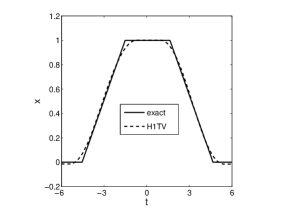
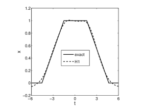
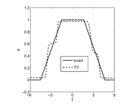
$H^{1}$-$TV$ sol. with $\boldsymbol{\eta}_{\mathrm{b}}$	$H^{1}$ sol. with $\eta_{\mathrm{h1}}$	$TV$ sol. with $\eta_{\mathrm{tv}}$

Figure 1: Numerical results for Example 1 with $5\%$ noise.

The numerical results are summarized in Table 1. In the table, the subscripts $\mathrm{b}$ and $\mathrm{o}$ refer to the balancing principle and the optimal choice, i.e., the value giving the smallest reconstruction error, respectively. The results for single-parameter models are indicated by subscripts $\mathrm{h1}$ and $\mathrm{tv}$, and the respective penalty parameter shown in Table 1 is the optimal one. The accuracy of the results is measured by the relative $L^{2}$ error $e=\|x-x^{\dagger}\|/\|x^{\dagger}\|$. A first observation is that the error $e_{\mathrm{b}}$, by the balancing principle for the proposed model $H^{1}$-$TV$ is smaller than the optimal choice for either $H^{1}$ or $TV$ penalty. This illustrates clearly the benefit of using multi-parameter model. Interestingly, the balancing principle gives an error fairly close to the optimal one, and the error decreases as the noise level decreases.

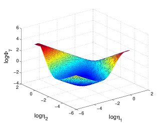
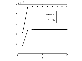
$\Phi_{\gamma}(\boldsymbol{\eta})$	convergence of Algorithm II

Figure 2: Numerical results for Example 1 with $5\%$ noise.

The numerical results for Example 1 with $\varepsilon=5\%$ noise is shown in Fig. 1. In particular, the classical $H^{1}$ smoothness penalty fails to restore the flat region satisfactorily, whereas the $TV$ approach suffers from stair-case effect in the gray region and reduced magnitude in the flat region, see Fig. 1. In contrast, the proposed $H^{1}$-$TV$ model can preserve the magnitude of flat region while reconstruct the gray region excellently. Therefore, it indeed combines the strengths of both $H^{1}$ and $TV$ models, and is suitable for restoring images with both flat and gray regions. The criterion $\Phi_{\gamma}$ is numerically well-behaved: there is a distinct local minimum, and it is numerically easy to minimize, see Fig. 2. Finally, we would like to remark that the algorithm converge rapidly with the convergence achieved in five iterations, see Fig. 2.

4.2 $\ell^{1}$-$\ell^{2}$ model

Example 2.

The kernel $k$ is given by $k(s,t)=\tfrac{1}{4}\left(\tfrac{1}{16}+(s-t)^{2}\right)^{-\frac{3}{2}}$, the exact solution $x^{\dagger}$ consists of two bumps and it is shown in Fig. 3. The penalties are $\psi_{1}(x)=\|x\|_{\ell^{1}}$ and $\psi_{2}(x)=\frac{1}{2}\|x\|_{\ell^{2}}^{2}$ to retrieve the groupwise sparsity structure. The integration interval is $[0,1]$. The size of the problem is 100.

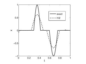
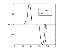
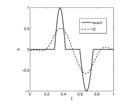
$\ell^{1}$-$\ell^{2}$ sol. with $\boldsymbol{\eta}_{\mathrm{b}}$	$\ell^{1}$ sol. with $\eta_{\mathrm{l1}}$	$\ell^{2}$ sol. with $\eta_{\mathrm{l2}}$

Figure 3: Numerical results for Example 2 with $5\%$ noise.

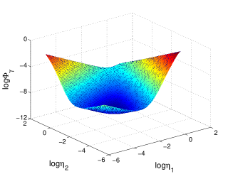
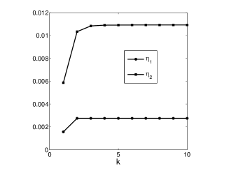
$\Phi_{\gamma}(\boldsymbol{\eta})$	convergence of Algorithm II

Figure 4: Numerical results for Example 2 with $5\%$ noise.

Table 2: Numerical results for Example 2.

$\epsilon$	$\boldsymbol{\eta}_{\mathrm{b}}$	$\boldsymbol{\eta}_{\mathrm{o}}$	$\eta_{\mathrm{l1}}$	$\eta_{\mathrm{l2}}$	$e_{\mathrm{b}}$	$e_{\mathrm{o}}$	$e_{\mathrm{l1}}$	$e_{\mathrm{l2}}$
5e-2	(2.75e-3,1.09e-2)	(3.16e-3,1.32e-3)	2.96e0	3.34e-3	4.18e-1	8.72e-2	1.04e0	4.59e-1
5e-3	(9.16e-5,2.86e-4)	(2.46e-4,1.07e-4)	1.03e-4	3.06e-5	2.09e-1	1.24e-2	8.97e-1	2.90e-1
5e-4	(2.82e-6,7.48e-6)	(2.34e-5,1.14e-5)	1.30e-5	4.08e-6	5.76e-2	7.98e-3	6.18e-1	2.17e-1
5e-5	(8.89e-8,2.26e-7)	(2.27e-6,1.06e-6)	1.24e-6	3.84e-8	1.57e-2	4.71e-3	4.85e-1	1.66e-1
5e-6	(2.79e-9,7.07e-9)	(1.66e-7,1.03e-7)	4.12e-9	1.41e-9	1.27e-2	2.27e-3	2.61e-1	9.55e-2

The numerical results for this example are show in Table 2 and Fig. 3. Here we are interested in the group structure of the solution with minimal number of influencing factors (nonzero coefficients). Again, we observe that the elastic-net compares favorably with the conventional $\ell^{1}$ and $\ell^{2}$ penalties in terms of the error, and the balancing principle can give reasonable estimate for the optimal choice. The conventional $\ell^{2}$ solution contains almost no zero entries, and thus it fails to distinguish between influencing and noninfluencing coefficients, i.e., identifying relevant factors. This difficulty is partially remedied by the $\ell^{1}$ model in that many entries of the $\ell^{1}$ solution are zero. Therefore, some relevant factors are correctly identified. However, it tends to select only some instead of all relevant factors, i.e., group structure. The elastic-net model combines the best of both $\ell^{1}$ and $\ell^{2}$ models, and it achieves the desired goal of identifying the group structure. Moreover, the magnitude assigned to the coefficients are reasonable compared to others. The algorithm converges quickly within five iterations.

4.3 2D image deblurring

Example 3.

The penalties are $\psi_{1}(x)=\|x\|_{\ell^{1}}$ and $\psi_{2}(x)=\frac{1}{2}\|x\|_{\ell^{2}}^{2}$. The kernel $k$ performs standard Gaussian blur with standard deviation $1$ and blurring width $5$. The exact solution $x^{\dagger}$ is shown in Fig. 5. The size of the image is $50\times 50$.

exact $x^{\dagger}$	$\ell^{1}$-$\ell^{2}$ sol. with $\boldsymbol{\eta}_{\mathrm{o}}=$(1.25e-2,1.29e-3)
$\ell^{1}$-$\ell^{2}$ sol. with $\boldsymbol{\eta}_{\mathrm{b}}=$(1.14e-3, 1.12e-3)	$\ell^{1}$ sol. with $\eta_{\mathrm{l1}}$=5.30e-1	$\ell^{2}$ sol. with $\eta_{\mathrm{l2}}=$3.31e-3

Figure 5: Numerical results for Example 3 with $1\%$ noise.

This example showcases a more realistic problem of image deblurring. Here one half of the data points are retained. The reconstructions for $1\%$ noise are shown in Fig. 5. The $\ell^{1}$ solution is more spiky, and neighboring pixels more or less act independently. In particular, due to missing data, there are some missing pixels in the blocks and the cross to be recovered. In contrast, the $\ell^{2}$ solution is more blockwise, but there are many nonzero coefficients indicated by the small spurious oscillations in the background. The elastic-net model achieves the best of the two: retaining the block structure with only fewer spurious nonzero coefficients. This is deemed important in medical imaging, e.g., classification. The numbers are more telling: $e_{\mathrm{b}}=2.99\times 10^{-1}$, $e_{\mathrm{o}}=2.44\times 10^{-1}$, $e_{\mathrm{l1}}=9.21\times 10^{-1}$, and $e_{\mathrm{l2}}=3.42\times 10^{-1}$. Therefore, the error $e_{\mathrm{b}}$ for elastic-net agrees well with the optimal choice, and it is smaller than that with the optimal choices for both $\ell^{1}$ and $\ell^{2}$ models.

5 Concluding remarks

We have studied theoretical properties of multi-parameter Tikhonov regularization. Some properties, e.g., monotonicity, concavity, asymptotic and differentiability, of the value function, were established. The discrepancy principle is partially justified in terms of consistency and convergence rates, however, the regularization parameter is not uniquely determined, which partially limits its practical application. It is of interest to develop auxiliary rules, which is currently under investigation. In contrast, the balancing principle allows justifications in terms of a posteriori error estimate and efficient numerical implementation. The numerical experiments show that multi-parameter models can significantly improve the reconstruction quality and the balancing principle can give reasonable results in comparison with the optimal choice in a computationally efficient way. The two proposed algorithms for computing the parameters of the balancing principle deliver excellent convergence behavior. However, a rigorous convergence analysis remains to be established.

References

- [1] M. Belge, M. E. Kilmer, and E. L. Miller. Efficient determination of multiple regularization parameters in a generalized L-curve framework. Inverse Problems, 18(4):1161–1183, 2002.
- [2] C. Brezinski, M. Redivo-Zaglia, G. Rodriguez, and S. Seatzu. Multi-parameter regularization techniques for ill-conditioned linear systems. Numer. Math., 94(2):203–228, 2003.
- [3] D. H. Brooks, G. F. Ahmad, R. S. Macleod, and G. M. Maratos. Inverse electrocardiography by simultaneous imposition of multiple constraints. IEEE Trans. Biomed. Eng., 46(1):3–18, 1999.
- [4] Z. Chen, Y. Lu, Y. Xu, and H. Yang. Multi-parameter Tikhonov regularization for linear ill-posed operator equations. J. Comput. Math., 26(1):37–55, 2008.
- [5] C. De Mol, E. De Vito, and L. Rosasco. Elastic-net regularization in learning theory. J. Complexity, 25(2):201–230, 2009.
- [6] H. W. Engl, M. Hanke, and A. Neubauer. Regularization of Inverse Problems. Kluwer, Dordrecht, 1996.
- [7] K. Ito, B. Jin, and T. Takeuchi. A regularization parameter for nonsmooth Tikhonov regularization. Technical Report UTMS 2010-3, Graduate School of Mathematical Sciences, University of Tokyo, 2010.
- [8] K. Ito, B. Jin, and J. Zou. A new choice rule for regularization parameters in Tikhonov regularization. Appl. Anal., page in press, 2010.
- [9] B. Jin, D. A. Lorenz, and S. Schiffler. Elastic-net regularization: error estimates and active set methods. Inverse Problems, 25(11):115022 (26pp), 2009.
- [10] B. Jin and J. Zou. Augmented Tikhonov regularization. Inverse Problems, 25(2):025001, 25, 2009.
- [11] B. Jin and J. Zou. Iterative parameter choice by discrepancy principle. Technical Report 2010-02(369), Department of Mathematics, Chinese University of Hong Kong, 2010.
- [12] S. Lu and S. V. Pereverzev. Multi-parameter regularization and its numerical regularization. Numer. Math., doi: 10.1007/s00211-010-0318-3.
- [13] S. Lu, S. V. Pereverzev, Y. Shao, and U. Tautenhahn. Discrepancy curves for multi-parameter regularization. J. Inv. Ill-Posed Probl., 18(6):655–676, 2010.
- [14] Y. Lu, L. Shen, and Y. Xu. Multi-parameter regularization methods for high-resolution image reconstruction with displacement errors. IEEE Trans. Circuits Syst. I. Regul. Pap., 54(8):1788–1799, 2007.
- [15] P. Mathé. The Lepskii principle revisited. Inverse Problems, 22(3):L11–L15, 2006.
- [16] V. A. Morozov. On the solution of functional equations by the method of regularization. Sov. Math. Dokl., 7:414–417, 1966.
- [17] I. M. Stephanakis. Regularized image restoration in multiresolution spaces. Opt. Eng., 36(6):1738–1744, 1997.
- [18] A. N. Tikhonov and V. Y. Arsenin. Solutions of Ill-Posed Problems. John Wiley, New York, 1977.
- [19] P. Xu, Y. Fukuda, and Y. Liu. Multiple parameter regularization: numerical solutions and applications to the determination of geopotential from precise satellite orbits. J. Geod., 80(1):17–27, 2006.
- [20] H. Zou and T. Hastie. Regularization and variable selection via the elastic net. J. R. Stat. Soc. Ser. B, 67(2):301–320, 2005.