f(R) Gravity and Maxwell Equations from the Holographic Principle

Abstract

Extending the holographic program of [1], we derive f(R) gravity and the Maxwell equations from the holographic principle, using time-like holographic screens. We find that to derive the Einstein equations and f(R) gravity in a natural holographic approach, the quasi-static condition is necessary. We also find the surface stress tensor and the surface electric current, surface magnetic current on a holographic screen for f(R) gravity and Maxwell’s theory, respectively.

1 Introduction

Gravity may not be a fundamental force, this may be related to a deep principle underlying the working of our world: The holographic principle. The most recent concrete proposal for a macroscopic picture of gravity is due to Verlinde [2] (see also [3]), which in turn is motivated by the gauge/gravity correspondence in string theory and an earlier proposal of Jacobson [4].

However, there are problems with the Verlinde’s proposal, as pointed out in [1]. First, Verlinde’s derivation of the Einstein equations always requires a positive temperature on a holographic screen, this is not attainable for an arbitrary screen. To avoid this problem, we propose to use a screen stress tensor to replace the assumption of equal partition of energy. Second, using Verlinde’s proposal, we do not have a reasonable holographic thermodynamics, there is always an area term in the holographic entropy of a gravitational system. There is no such problem in our proposal. A prediction of the program of [1] is that there is always a huge holographic entropy associated to a gravitational system, with a form similar to the Bekenstein bound.

In this paper, we would like to clarify the role of the adiabatic condition used in [1] left unexplained in that paper. To see how far our program can get, we also use the same idea to derive f(R) gravity, we see that unlike Verlinde’s proposal in which it is impossible to accommodate theories containing higher derivatives [6], there is a natural ansatz for the surface stress tensor to derive the f(R) theory.

Lastly, using the same idea with a surface current replacing the surface stress tensor, we derive the Maxwell equations. Our success demonstrates that our program is more universal.

This paper is organized as follows. In sect.2, we review our holographic derivation of the Einstein equations on a time-like screen. In sect.3 and sect.4, we derive the f(R) equations and the Maxwell equations in a similar holographic approach, respectively. We conclude in sect.5.

2 Einstein equations from the holographic principle

In this section, we shall review our derivation of the Einstein equations in a holographic program [1] different from Verlinde’s [2]. We will explain the physical reason to impose the quasi-static condition used in the previous paper [1] in order to derive the Einstein equations naturally on a time-like holographic screen.

Let us start with some definitions. Our holographic screen is a 2+1 dimensional time-like hyper-surface $\Sigma$, which can be open or closed, embedded in the 3+1 dimensional space-time $M$. We use $x^{a}$, $g_{ab}$, $\nabla_{a}$, $y_{i}$, $\gamma_{ij}$ and $D_{i}$ (here $a$, $b$ run from 0 to 3, and $i$, $j$ run from 0 to 2) to denote the coordinates, metric and covariant derivatives on $M$ and $\Sigma$, respectively.

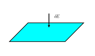
Figure 1: An energy flux $\delta E$ passing through an open patch on the holographic screen.

Unlike Jacobson’s idea [4], we consider an energy flux $\delta E$ passing through an open patch on a time-like holographic screen $d\Sigma=dAdt$ (see Fig. 1)

$$\delta E=\int_{\Sigma}T_{ab}\xi^{a}N^{b}dAdt,$$ (1)

where $T_{ab}$ is the stress tensor of matter in the bulk $M$, $\xi^{a}$ is a time-like Killing vector, and $N^{a}$ is the unit vector normal to $\Sigma$. To define $N^{a}$ we may assume $\Sigma$ be specified by a function

$$f_{\Sigma}(x^{a})=c.$$ (2)

Thus, the normalized normal vector to $\Sigma$ is

$$N^{a}=\frac{g^{ab}\nabla_{b}f_{\Sigma}}{\sqrt{\nabla_{b}f_{\Sigma}\nabla^{b}f_{\Sigma}}}.$$ (3)

As in [1], we introduce the surface energy density $\sigma$ and the surface energy flux $j$ on the screen. These are quantities contained in the surface stress tensor $\tau^{ij}$ and given by

$$\sigma=u_{i}\tau^{ij}\xi_{j}\ ,\ j=-m_{i}\tau^{ij}\xi_{j},$$ (4)

where $u_{i}$, $m_{i}$ are the unit vectors normal to the screen’s boundary $\partial\Sigma$ (we will give the expressions of $u_{i}$ and $m_{i}$ shortly), $\xi_{i}$ is a Killing vector on $\Sigma$. In a quasi-static space-time $u^{i}$ is related to $\xi^{i}$ by $u^{i}=e^{-\phi}\xi^{i}$, and $\phi$ is the Newton’s potential defined by $\phi=\frac{1}{2}\log(-\xi^{i}\xi_{i})$ on the screen. Note that $\sigma$ and $j$ are the energy density and energy flux on the screen measured by the observer at infinity. Apparently, central to our discussion is the choice of $\tau_{ij}$. Naturally, $\tau^{ij}$ should depend on the extrinsic geometry of the screen, since extrinsic geometry contains both the information of the bulk $M$ and of the screen $\Sigma$, thus it is a natural bridge relating both sides to realize the holographic principle. Thus we assume the following simplest and most general form

$$\tau^{ij}=nK^{ij}+q\gamma^{ij},$$ (5)

where $n$ is a constant, $q$ is a function to be determined and $K^{ij}$ is the extrinsic curvature on $\Sigma$ defined by

$$K_{ij}=-e^{a}_{i}e^{b}_{j}\nabla_{a}N_{b},$$ (6)

where $e^{b}_{j}=\frac{\partial x^{a}}{\partial y^{i}}$ is the projection operator satisfying $N_{a}e^{a}_{i}=0$.

On the screen, the change of energy has two sources, one is due to variation of the energy density $\sigma$, the other is due to energy flowing out the patch to other parts of the screen, given by the energy flux $j$. The energy variation on the patch is then given by

$$\delta E = \int(u_{i}\tau^{ij}\xi_{j})dA|^{t+dt}_{t}-\int m_{i}\tau^{ij}\xi_{j}dydt$$ (7)

$$= -\int_{\partial\Sigma}(M_{i})\tau^{ij}\xi_{j}\sqrt{h}dz^{2}=-\int_{\Sigma}D_{i}(\tau^{ij}\xi_{j})dAdt,$$

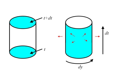
Figure 2: Left panel: The first term $\int(u_{i}\tau^{ij}\xi_{j})dA|^{t+dt}_{t}$ in Eq.(7) is due to change of the density. Right panel: The second term $-\int m_{i}\tau^{ij}\xi_{j}dydt$ is the energy flow (denoted by the red arrows) through the patch boundary parameterized by $y$.

where the first term in the first equality is due to change of the density and the second term is the energy flow through the patch boundary parameterized by $y$ (see Fig. 2). These two terms can be naturally written in a uniform form, since the boundary of the patch consists of two space-like surfaces ($d\Sigma$ at $t$ and $t+dt$), and a time-like boundary. $h$ is the determinant of the reduced metric on $\partial\Sigma$, $D_{i}$ is the covariant derivative on $\Sigma$. $M_{i}$ is a unit vector in $\Sigma$ and is normal to $\partial\Sigma$. Let us choose a suitable function $f_{\partial\Sigma}(y^{i})=c$ on $\Sigma$ to denote the boundary $\partial\Sigma$, then we have

$$M^{i}=\frac{\gamma^{ij}D_{j}f_{\partial\Sigma}}{\sqrt{D_{j}f_{\partial\Sigma}D^{j}f_{\partial\Sigma}}}.$$ (8)

Notice that when $M^{i}$ is along the direction of $dy^{0}$($dt$) it becomes $u^{i}$, and when along the direction of $dy^{i}$($dy^{1},dy^{2}$) it becomes $m^{i}$.

For a reason to be clear later, we focus on a quasi-static process in the following derivations. Recall that in Eq.(2) we use $f_{\Sigma}(x^{a})=c$ to denote the holographic screen $\Sigma$. In the quasi-static limit, $f_{\Sigma}(x^{a})$ is independent of time, so $N_{a}\sim(0,\partial_{1}f_{\Sigma},\partial_{2}f_{\Sigma},\partial_{3}f_{\Sigma})$. Note that $\xi^{a}\simeq(1,0,0,0)$ in the quasi-static limit, thus we have $N_{a}\xi^{a}\rightarrow 0$. The Killing vector $\xi_{i}$ on $\Sigma$ can be induced from the Killing vector $\xi_{a}$ in the bulk $M$ in the quasi-static limit:

$$\xi_{i}=\xi_{a}e^{a}_{i},\ \ D_{(i}\xi_{j)}=\nabla_{a}(\xi_{b}-N_{c}\xi^{c}N_{b})e^{a}_{(i}e^{b}_{j)}=K_{ij}N_{a}\xi^{a}\rightarrow 0.$$ (9)

From Eq.(5) and the Gauss-Codazzi equation $R_{ab}N^{a}e^{b}_{i}=-D_{j}(K^{j}\ _{i}-K\gamma^{j}\ _{i})$, one can rewrite Eq.(7) as

$$\delta E = \int_{\Sigma}[nR_{ab}\xi^{i}e^{a}_{i}N^{b}-\xi^{i}D_{i}(nK+q)]dAdt$$ (10)

$$= \int_{\Sigma}[nR_{ab}\xi^{a}N^{b}-\xi^{a}\nabla_{a}(nK+q)]dAdt,$$

where we have used the formulas $\xi^{a}=\xi^{i}e^{a}_{i}$, $\xi^{i}D_{i}f=\xi^{a}\nabla_{a}f$ in the quasi-static limit. It should be stress that the second term $\xi^{a}\nabla_{a}(nK+q)$ in Eq.(10) can not be written in the form $\xi^{a}N^{b}B_{ab}$ ($B_{ab}$ is independent of $\xi^{a}$ and $N^{b}$). For details, please refer to the Appendix.

Take into consideration that $\xi^{a}$, $N^{b}$ are independent vectors and $g_{ab}\xi^{a}N^{b}=0$, equating Eq.(1) and Eq.(10) results in

$$nR_{ab}+fg_{ab}=T_{ab},\ \ \ q=-nK,$$ (11)

where $f$ is an arbitrary function. We note that the second equation is a consequence of the fact that the second term on the R.H.S. of Eq.(10) must be vanishing. This result tells us that the surface stress tensor is the same as the Brown-York surface stress tensor, but we have not made use of any action. Using the energy conservation equation $\nabla^{a}T_{ab}=0$, we obtain $f=n(-\frac{R}{2}+\Lambda)$. Defining the Newton’s constant as $G=\frac{1}{8\pi n}$, we then get the Einstein equations

$$R_{ab}-\frac{R}{2}g_{ab}+\Lambda g_{ab}=8\pi GT_{ab}.$$ (12)

Substituting $n=\frac{1}{8\pi G}$ and $q=-nK$ into Eq.(5), we obtain

$$\tau^{ij}=\frac{1}{8\pi G}(K^{ij}-K\gamma^{ij}),$$ (13)

this is just the quasi-local stress tensor of Brown-York defined in [8]. Now we have derived the Einstein equations and the Brown-York stress tensor from our holographic program.

In the above derivations, for simplicity, we have imposed the quasi-static condition $N_{a}\xi^{a}=0$. We now briefly discuss the relation between the quasi-static condition and the holographic principle. Let us try to see what will happen when we abandon the quasi-static condition $N_{a}\xi^{a}=0$. The energy flux $\delta E$ passing through an open patch on the holographic screen $d\Sigma=dAdt$ becomes

$$\delta E=\int_{\Sigma}T_{ab}\xi^{a}N^{b}dAdt=\int_{\Sigma}[T_{ab}e^{a}_{i}\xi^{i}N^{b}+T_{ab}N^{a}N^{b}(N_{c}\xi^{c})]dAdt,$$ (14)

a new term $T_{ab}N^{a}N^{b}(N_{c}\xi^{c})$ which is proportional to the pressure along the direction of $N^{a}$ appears. Since now we aim to study the relationship between the quasi-static condition and the holographic principle, not to derive the Einstein equations, for simplicity, we assume that the Einstein equations are satisfied and so the surface stress tensor $\tau_{ij}$ is the Brown-York stress tensor Eq.(13). Then, Eq.(14) is expected to be

$$\delta E = \int_{\Sigma}\frac{1}{8\pi G}[R_{ab}e^{a}_{i}\xi^{i}N^{b}+(R_{ab}-\frac{R}{2}g_{ab})N^{a}N^{b}(N_{c}\xi^{c})]dAdt$$ (15)

$$= \int_{\Sigma}[-\xi_{j}D_{i}\tau^{ij}+\frac{1}{16\pi G}(-^{(3)}R+K^{2}-K_{ij}K^{ij})(N_{c}\xi^{c})]dAdt.$$

We have used the Gauss-Godazzi equations

$$R_{ab}N^{a}e^{b}_{i}=-D_{j}(K^{j}\ _{i}-K\delta^{j}\ _{i}),$$

$$(2R_{ab}-Rg_{ab})N^{a}N^{b}=-^{(3)}R+K^{2}-K_{ij}K^{ij},$$ (16)

where ${}^{(3)}R$ is the Ricci scalar on $\Sigma$.

Note that $\xi_{i}=e^{a}_{i}\xi_{a}$ is on longer a Killing vector on the screen, since $D_{(i}\xi_{j)}=K_{ij}N_{a}\xi^{a}\neq 0$. If we still assume Eq.(4) with $\xi_{i}$ being the projection of $\xi^{a}$ on $\Sigma$, the change of energy on screen Eq.(7) becomes

$$\delta E = \int(u_{i}\tau^{ij}\xi_{j})dA|^{t+dt}_{t}-\int m_{i}\tau^{ij}\xi_{j}dydt$$

$$= -\int_{\partial\Sigma}(M_{i})\tau^{ij}\xi_{j}\sqrt{h}dz^{2}=-\int_{\Sigma}D_{i}(\tau^{ij}\xi_{j})dAdt$$

$$= \int_{\Sigma}[-\xi_{j}D_{i}\tau^{ij}-\tau^{ij}D_{i}\xi_{j}]dAdt$$

$$= \int_{\Sigma}[-\xi_{j}D_{i}\tau^{ij}+\frac{1}{8\pi G}(K^{2}-K^{ij}K_{ij})(N_{c}\xi^{c})]dAdt$$

Since $-^{(3)}R-K^{2}+K^{ij}K_{ij}\neq 0$, the second term of Eq.(15) is not equal to the second term of Eq.(2) except when $N_{c}\xi^{c}=0$. Of course, one can add some terms to Eq.(2) to equate Eq.(15) and Eq.(2), but it is very unnatural. So if we expect the holographic principle to require that the the energy flow through the holographic screen (defined by Eq.(15)) and the change of energy on the holographic screen (defined by Eq.(2)) are equal to each other, the quasi-static condition $(N_{a}\xi^{a}\rightarrow 0)$ is necessary.

Finally, even without using the Einstein equation, the fact that the second term in Eq.(14) is proportional to the transverse component of $T_{ab}$ tells us that we need to introduce an transeverse term in the surface stress tensor, this is not holographic at all.

3 f(R) gravity from the holographic principle

In this section, we shall derive the equations of f(R) gravity in the same manner as in [1] and the previous section. For the same reason as in the presiouc section we impose the quasi-static condition $(N_{a}\xi^{a}\rightarrow 0)$.

The energy flux $\delta E$ passing through an open patch on the holographic screen $d\Sigma=dAdt$ and the change of energy on the screen take the same form as in Eq.(1) and Eq.(7)

$$\delta E=\int_{\Sigma}T_{ab}\xi^{a}N^{b}dAdt,$$ (18)

$$\delta E = \int(u_{i}\tau^{ij}\xi_{j})dA|^{t+dt}_{t}-\int m_{i}\tau^{ij}\xi_{j}dydt$$ (19)

$$= -\int_{\partial\Sigma}(M_{i})\tau^{ij}\xi_{j}\sqrt{h}dz^{2}=-\int_{\Sigma}D_{i}(\tau^{ij}\xi_{j})dAdt.$$

The only difference is the assumption of surface stress tensor $\tau^{ij}$. As argued in Sect.2, $\tau^{ij}$ should depend on the the extrinsic geometry of the screen, since it is a natural bridge relating the bulk $M$ and the holographic screen $\Sigma$. Instead of the simplest assumption Eq.(5), we now assume more generally

$$\tau^{ij}=nf^{\prime}(R)K^{ij}+q\gamma^{ij},$$ (20)

where $f^{\prime}(R)$ is a general function of the Ricci scalar $R$, and $q$ is to be determined. The case $f^{\prime}(R)=1$ is special and is what underlying the Einstein equations. Substituting Eq.(20) into Eq.(19), we obtain

$$\delta E = -\int_{\Sigma}D_{i}(\tau^{ij}\xi_{j})dAdt$$

$$= \int_{\Sigma}(nf^{\prime}R_{ab}N^{a}\xi^{b}-n\xi^{a}K_{ab}\nabla^{b}f^{\prime}-\xi^{a}\nabla_{a}(q+nf^{\prime}K))dAdt$$

$$= \int_{\Sigma}(nf^{\prime}R_{ab}N^{a}\xi^{b}+n\xi^{a}\nabla_{a}N_{b}\nabla^{b}f^{\prime}-\xi^{a}\nabla_{a}(q+nf^{\prime}K))dAdt$$

$$= \int_{\Sigma}[nN^{a}\xi^{b}(R_{ab}f^{\prime}-\nabla_{a}\nabla_{b}f^{\prime})+\xi^{a}\nabla_{a}(nN^{b}\nabla_{b}f^{\prime}-nf^{\prime}K-q)]dAdt.$$

In the above calculation, we have used the Gauss-Codazzi equation $R_{ab}N^{a}e^{b}_{i}=-D_{j}(K^{j}\ _{i}-K\gamma^{j}\ _{i})$, $\xi^{a}\nabla_{a}R=0$, $\xi^{a}K_{ab}=-\xi^{a}\nabla_{a}N_{b}$ and the quasi-static condition $(N_{a}\xi^{a}\rightarrow 0)$. As the case in Sect.2 the second term of Eq.(3) $\xi^{a}\nabla_{a}(nN^{b}\nabla_{b}f^{\prime}-nf^{\prime}K-q)$ does not contain term $\xi^{a}N^{b}B_{ab}$, where $B_{ab}$ is independent of $\xi^{a}$ and $N^{b}$. For details, please refer to the Appendix (just replace $(nK+q)$ by $(nf^{\prime}K+q-nN^{b}\nabla_{b}f^{\prime})$.

Since $\xi^{a}$, $N^{b}$ are independent vectors and $g_{ab}\xi^{a}N^{b}=0$, equating Eq.(18) and Eq.(3) results in

$$q=nN^{b}\nabla_{b}f^{\prime}-nf^{\prime}K,\$$

$$f^{\prime}R_{ab}-\nabla_{a}\nabla_{b}f^{\prime}+Fg_{ab}=\frac{1}{n}T_{ab},$$ (22)

where $F$ is an arbitrary function, using $\nabla_{a}T^{ab}=0$, we get

$$\nabla^{b}F=\nabla^{b}(\nabla_{c}\nabla^{c}f^{\prime}-\frac{f}{2}).$$ (23)

Thus, $F=\Box f^{\prime}-\frac{f}{2}+\Lambda$. Define the Newton’s constant as $G=\frac{1}{8\pi n}$, we then obtain equations of motion of f(R) gravity

$$f^{\prime}R_{ab}-\frac{f}{2}g_{ab}-\nabla_{a}\nabla_{b}f^{\prime}+g_{ab}\Box f^{\prime}+\Lambda g_{ab}=8\pi GT_{ab}.$$ (24)

Substituting $q=\frac{1}{8\pi G}(N^{b}\nabla_{b}f^{\prime}-f^{\prime}K)$ into Eq.(20), we get the surface stress tensor of f(R) gravity

$$\tau^{ij}=\frac{1}{8\pi G}[f^{\prime}(R)(K^{ij}-K\gamma^{ij})+N^{c}\nabla_{c}f^{\prime}\gamma^{ij}].$$ (25)

Now, we have obtained the f(R) equations and surface stress tensor from our holographic program. Let us continue to understand the physical meaning of the surface stress tensor Eq.(25). It is well known that the action of f(R) gravity

$$S=\frac{1}{2\kappa}\int d^{4}x\sqrt{-g}f(R)+S_{M}(g_{ab},\psi)$$ (26)

is equivalent to the Einstein gravity with a scalar field

$$S=\int d^{4}x\sqrt{-\tilde{g}}[\frac{\tilde{R}}{2\kappa}-\frac{1}{2}\partial^{a}\tilde{\phi}\partial_{a}\tilde{\phi}-V(\tilde{\phi})]+S_{M}(e^{-\sqrt{2\kappa/3}}\tilde{g_{ab}},\psi),$$ (27)

if we perform conformal transformation $\tilde{g}_{ab}=f^{\prime}g_{ab}$ and $\tilde{\phi}=\sqrt{\frac{3}{2\kappa}}\ln f^{\prime}$, $V(\tilde{\phi})=\frac{Rf^{\prime}-f}{2\kappa(f^{\prime})^{2}}$. The surface stress tensor for metric $\tilde{g_{ab}}$ is

$$\tilde{\tau}^{ij}=\frac{1}{\kappa}(\tilde{K}^{ij}-\tilde{K}\tilde{\gamma}^{ij}).$$ (28)

Note that $\tilde{N}_{a}=(f^{\prime})^{1/2}N_{a}$, $\tilde{N}^{a}=(f^{\prime})^{-1/2}N^{a}$, $\tilde{\gamma}_{ab}=f^{\prime}\gamma_{ab}$ and $\tilde{\Gamma}^{d}_{cb}=\Gamma^{d}_{cb}+C^{d}_{cb}$, where $C^{d}_{cb}=\frac{1}{2f^{\prime}}(\delta^{d}_{c}\nabla_{b}f^{\prime}+\delta^{d}_{b}\nabla_{c}f^{\prime}-g_{cb}g^{de}\nabla_{e}f^{\prime})$. After some calculation, we find

$$\tilde{\tau}_{ij} = \frac{(f^{\prime})^{1/2}}{\kappa}(K_{ij}-K\gamma_{ij})+\frac{(f^{\prime})^{-1/2}}{\kappa}\gamma_{ij}N^{d}\nabla_{d}f^{\prime}$$ (29)

$$= (f^{\prime})^{-1/2}\tau_{ij}.$$

It is interesting that the surface stress tensors $\tilde{\tau}_{ij}$ and $\tau_{ij}$ of Eq.(25) are related exactly by an conformal factor $(f^{\prime})^{-1/2}$. Let us move on to understand this conformal factor $(f^{\prime})^{-1/2}$. Firstly, let us derive some useful formulas.

$$\tilde{T}^{M}_{ab}=-2\frac{1}{\sqrt{-\tilde{g}}}\frac{\delta S_{M}}{\delta\tilde{g}^{ab}}=\frac{1}{f^{\prime}}T^{M}_{ab}$$

$$\tilde{T}^{\tilde{\phi}}_{ab}=\tilde{\nabla}_{a}\tilde{\phi}\tilde{\nabla}_{b}\tilde{\phi}-\frac{1}{2}\tilde{g}_{ab}\tilde{g}^{cd}\tilde{\nabla}_{c}\tilde{\phi}\tilde{\nabla}_{d}\tilde{\phi}-\tilde{g}_{ab}V(\tilde{\phi})$$

$$\tilde{N}_{a}=(f^{\prime})^{1/2}N_{a},\ \tilde{\gamma}_{ab}=\tilde{g}_{ab}-\tilde{N}_{a}\tilde{N}_{b}=f^{\prime}\gamma_{ab}$$

$$\tilde{M}_{i}=(f^{\prime})^{1/2}M_{i},\ \tilde{h}_{ij}=\tilde{\gamma}_{ij}-\tilde{M}_{i}\tilde{M}_{j}=f^{\prime}h_{ij}$$

$$\tilde{\xi}^{a}=\xi^{a}$$ (30)

We shall prove the last equation $\tilde{\xi}^{a}=\xi^{a}$ below. Assume $\xi^{a}$ be a Killing vector of the metric $g_{ab}$, we have

$$L_{\xi}g_{ab}=\xi^{c}\partial_{c}g_{ab}+(\partial_{a}\xi^{c})g_{cb}+(\partial_{b}\xi^{c})g_{ca}=0,$$ (31)

then

$$L_{\xi}\tilde{g}_{ab} = \xi^{c}\partial_{c}(f^{\prime}g_{ab})+f^{\prime}(\partial_{a}\xi^{c})g_{cb}+f^{\prime}(\partial_{b}\xi^{c})g_{ca}$$ (32)

$$= g_{ab}\xi^{c}\partial_{c}f^{\prime}+f^{\prime}(\xi^{c}\partial_{c}g_{ab}+(\partial_{a}\xi^{c})g_{cb}+(\partial_{b}\xi^{c})g_{ca})$$

$$= 0,$$

where we have used the identity $\xi^{a}\nabla_{a}R=0$. Now, it is clear that $\xi^{a}$ is also a Killing vector of $\tilde{g}_{ab}$. The energy flux $\delta E$ passing through the holographic screen is

$$\delta\tilde{E} = \int_{\Sigma}(\tilde{T}^{M}_{ab}+\tilde{T}^{\tilde{\phi}}_{ab})\xi^{a}\tilde{N}^{b}\sqrt{-\tilde{\gamma}}d^{2}xdt$$ (33)

$$= \int_{\Sigma}\tilde{T}^{M}_{ab}\xi^{a}\tilde{N}^{b}\sqrt{-\tilde{\gamma}}d^{2}xdt$$

$$= \int_{\Sigma}T_{ab}\xi^{a}N^{b}\sqrt{-\gamma}d^{2}xdt$$

$$= \delta E.$$

Above we have used again the identity $\xi^{a}\nabla_{a}R=0$ and the quasi-static limit $(N_{a}\xi^{a}\rightarrow 0)$, so that $\tilde{T}^{\tilde{\phi}}_{ab}\xi^{a}\tilde{N}^{b}=0$.

The change of energy on the screen is

$$\delta\tilde{E} = -\int_{\partial\Sigma}\tilde{M}^{i}\tilde{\tau}_{ij}\xi^{j}\sqrt{\tilde{h}}d^{2}z=-\int_{\partial\Sigma}M^{i}(f^{\prime})^{1/2}\tilde{\tau}_{ij}\xi^{j}\sqrt{h}d^{2}z$$ (34)

Equating Eq.(33) and Eq.(34), we find

$$\delta E = -\int_{\partial\Sigma}M^{i}(f^{\prime})^{1/2}\tilde{\tau}_{ij}\xi^{j}\sqrt{h}d^{2}z$$ (35)

$$= -\int_{\partial\Sigma}M^{i}\tau_{ij}\xi^{j}\sqrt{h}d^{2}z$$

It is clear that $(f^{\prime})^{1/2}\tilde{\tau}_{ij}$ plays the rule of $\tau_{ij}$.

The above discussion is a check that from the holographic principle we have derived the correct surface stress tensor (25) of $f(R)$ gravity, and helps us to gain some insight into the physical meaning of f(R) surface stress tensor (25): It is related with it’s conformal counterpart by an appropriate conformal factor $\tau_{ij}=(f^{\prime})^{1/2}\tilde{\tau}_{ij}$.

4 Maxwell equations from the holographic principle

In this section, we shall derive the Maxwell equations in a similar holographic approach as in the above two sections. However, there are two main differences. First, instead of using conservation of energy, we use conservation of charge to derive the Maxwell equations. We calculate the charge passing through the holographic screen in the bulk $M$ and the charge change on the screen $\Sigma$ respectively, and equate them as dictated by the holographic principle. With an appropriate assumption of the current on the screen, we can obtain the Maxwell equations. Secondly, we do not need the quasi-static condition $(N_{a}\xi^{a}\rightarrow 0)$, in fact we make no use of a Killing vector in our derivations of the Maxwell equations, since a Killing vector is related to energy instead of charge.

Consider the electric charge $\delta Q$ passing through an open patch on the holographic screen $d\Sigma=dAdt$

$$\delta Q=\int_{\Sigma}J^{a}N_{a}dAdt,$$ (36)

where $J^{a}$ is electric current of matter in the bulk $M$. Assume the surface electric current on the screen be $j_{i}$, then the charge change on the screen is

$$\delta Q = \int u^{i}j_{i}|^{t+dt}_{t}-\int m^{i}j_{i}\sqrt{h}dydt$$ (37)

$$= -\int_{\partial\Sigma}M^{i}j_{i}\sqrt{h}dy^{2}=-\int_{\Sigma}D^{i}j_{i}dAdt,$$

where the first term in the first equality is due to change of charge density and the second term is the electric flow through the patch boundary parameterized by $y$. Again these two terms can be naturally written in a uniform form $-\int_{\partial\Sigma}M^{i}j_{i}\sqrt{h}dy^{2}$. Applying Stokes’s Theorem, we get the last equality.

According to the holographic principle, we should equate Eq.(36), the charge flow through the patch of the holographic screen, and Eq.(37), the charge change on this patch, yielding

$$D^{i}j_{i}=-N_{a}J^{a}.$$ (38)

So far, we have not made any assumption about the form of $j_{i}$. Now, let us gain some insight into the form of $j_{i}$ from Eq.(38). According to the holographic principle, we expect to derive the bulk equations of motion from Eq.(38), which implies that $j^{i}=e^{a}_{i}j^{a}$ should linearly depend on $N^{a}$. Thus, the general form for $j_{a}$ is

$$j_{a}=A_{ab}N^{b}+A_{abc}\nabla^{b}N^{c}+...$$ (39)

And $j_{a}$ must satisfy the following conditions

$$N^{a}j_{a}=0,\ \ D^{i}j_{i}=\gamma^{ab}\nabla_{a}j_{b}=-N_{a}J^{a},$$ (40)

where $\gamma^{ac}$ is the projection operator defined as $\gamma^{ac}=g^{ac}-N^{a}N^{c}$. For simplicity, we consider the simplest assumption $j_{a}=A_{ab}N^{b}$. The conditions Eq.(40) become

$$A_{ab}N^{a}N^{b}=0,\ \ (\gamma^{ac}\nabla_{a}A_{cb})N^{b}+\gamma^{c}_{a}A_{cb}\nabla^{a}N^{b}=-N^{b}J_{b}.$$ (41)

From the last equation of Eq.(41), we have

$$(\gamma^{ac}\nabla_{a}A_{cb}+J_{b})N^{b}=0,\ \gamma^{c}_{a}A_{cb}\nabla^{a}N^{b}=0$$ (42)

Since $\gamma^{c}_{a}\nabla^{a}N^{b}=-K^{cb}$ is symmetrical in $c$ and $b$, we derive $\gamma^{a}_{c}\gamma^{d}_{b}A_{ad}=-\gamma^{a}_{b}\gamma^{d}_{c}A_{ad}$ from $\gamma^{c}_{a}A_{cb}\nabla^{a}N^{b}=0$. For we can change the direction of $N^{a}$ arbitrarily with changing the screen, taking $\gamma^{a}_{c}\gamma^{d}_{b}A_{ad}=-\gamma^{a}_{b}\gamma^{d}_{c}A_{ad}$ and $A_{ab}N^{a}N^{b}=0$ into account, we find that $A_{ab}$ is antisymmetric. Thus, the first equation of Eq.(42) becomes

$$(\gamma^{ac}\nabla_{a}A_{cb}+J_{b})N^{b} = (\nabla_{a}A^{a}_{b}+J_{b})N^{b}-(N^{a}\nabla_{a}A_{cb})N^{c}N^{b}$$ (43)

$$= (\nabla_{a}A^{a}_{b}+J_{b})N^{b}=0.$$

So for arbitrary $N^{b}$, we get

$$\nabla_{a}A^{ab}=-J^{b},$$ (44)

with $A^{ab}$ an antisymmetric tensor and the surface electric current $j_{a}=A_{ab}N^{b}$ on the screen. Note that conservation of charge $\nabla_{a}J^{a}=0$ is satisfied automatically for antisymmetric $A^{ab}$

$$-\nabla_{a}J^{a}=\nabla_{a}\nabla_{b}A^{ab}=\frac{1}{2}(\nabla_{a}\nabla_{b}-\nabla_{b}\nabla_{a})A^{ab}=R_{ab}A^{ab}=0.$$ (45)

The above approach can be directly extended to the case of magnetic charge. Assume the magnetic current in the bulk and on the screen be $J^{a}_{m}=0$ and $j^{a}_{m}=B^{ab}N_{b}$, respectively. With the same procedure we arrive at

$$B^{ab}=-B^{ba},\ \ \nabla_{a}B^{ab}=-J^{b}_{m}=0.$$ (46)

Since the magnetic current $J^{b}_{m}=0$ in the bulk, it is expected that $j^{a}_{m}=B^{ab}N_{b}$ is not an independent physical quantity, it should either vanish or be related to the surface electric current $j^{a}$ on the screen. In view of the electromagnetical duality, it is natural to assume that the surface electric current and magnetic current on the screen are related with each other by the Hodge duality

$$B^{ab}=\frac{1}{2}\epsilon^{abcd}A_{cd}.$$ (47)

Then, Eq.(46) becomes

$$\epsilon^{abcd}\nabla_{b}A_{cd}=0,$$ (48)

which is just the Bianchi identity. The general solution of the above equation is $A_{cd}=\partial_{d}A_{c}-\partial_{c}A_{d}$ with $A_{c}$ an arbitrary vector field. Rename $A_{cd}$ by $F_{dc}$, let us summarize our results. The surface electric current and magnetic current on the screen are

$$j^{a}=F^{ba}N_{b},\ \ \ j^{a}_{m}=\frac{1}{2}\epsilon^{bacd}F_{cd}N_{b}.$$ (49)

The equations of motion in the bulk $M$ are

$$\nabla_{a}F^{ab}=J^{b},\ \ \nabla_{[a}F_{bc]}=0,$$ (50)

where $F_{ab}=\partial_{a}A_{b}-\partial_{b}A_{a}$ and $[\ \ ]$ denotes complete antisymmetrization. The above equations are just the Maxwell equations. Applying the formulas

$$F_{ab}\ ^{*}F^{bc}=\frac{1}{4}F\ ^{*}F\delta^{c}_{a},\ \ F_{ab}F^{bc}-\ ^{\ast}F_{ab}\ ^{\ast}F^{bc}=\frac{1}{2}F^{2}\delta^{c}_{a},$$ (51)

we obtain the following interesting identities

$$jj_{M}=-\frac{1}{4}F\ ^{*}F,\ \ j^{2}-j^{2}_{M}=-\frac{1}{2}F^{2},$$ (52)

where ${}^{*}F^{ab}$ is the Hodge duality of $F_{cd}$, ${}^{*}F^{ab}=\frac{1}{2}\epsilon^{abcd}F_{cd}$. Note that the L.H.S of Eqs.(52) are physical quantities on the screen while the R.H.S of Eqs.(52) contain only physical quantities in the bulk which are independent of the direction of the screen $N^{a}$, so $j^{a}$ and $j^{a}_{M}$ contain all the information of the bulk ($F^{2}$ and ${}^{*}FF$) which is a reflection of the holographic principle.

Now, we have derived the Maxwell equations from the holographic principle and an appropriate assumption for the relationship between the surface electric current and magnetic current on the holographic screen.

5 Conclusions

We have derived f(R) gravity and the Maxwell equations from the holographic program we proposed in [1]. We find the surface stress tensor and surface electric current, surface magnetic current for f(R) gravity and Maxwell’s theory, respectively. It is interesting to extend our holographic approach to more general higher derivative gravity, and investigate the corresponding thermodynamics on a time-like holographic screen. It should be mentioned that in Sect.4 we only find the simplest solution of Eqs.(39) and (40), whether there are other solutions and corresponding holographic electromagnetic theories is an interesting problem. We hope we will gain more insight into these problems in the future.

Appendix

In this appendix, we shall prove that the second term $\xi^{a}\nabla_{a}(nK+q)$ in Eq.(10) does not contain the term $\xi^{a}N^{b}B_{ab}$, where $B_{ab}$ is independent of $\xi^{a}$ and $N^{b}$. If $\xi^{a}\nabla_{a}(nK+g)$ does include such terms, $(nK+g)$ must depend on $N^{b}$ linearly

$$nK+g=A_{b}N^{b}+A_{bc}\nabla^{b}N^{c}+...$$ (53)

Thus,

$$\xi^{a}\nabla_{a}(nK+g) = \xi^{a}N^{b}\nabla_{a}A_{b}+\xi^{a}A^{b}\nabla_{a}N_{b}+(\xi^{d}\nabla_{d}A^{ab})\nabla_{a}N_{b}...$$ (54)

$$= \xi^{a}N^{b}\nabla_{a}A_{b}+\xi^{d}\nabla^{a}N^{b}(\nabla_{d}A_{ab}+g_{da}A_{b})+...$$

Take into consideration the fact that Eq.(1) does not contain the term $\xi^{d}\nabla^{a}N^{b}$ and that $R_{ab}$ is symmetrical, equating Eq.(1) and Eq.(10) yields

$$\nabla_{a}A_{b}=\nabla_{b}A_{a},$$ (55)

$$D_{i}A_{jk}+\gamma_{ij}A_{k}=e^{d}_{i}e^{a}_{j}e^{b}_{k}(\nabla_{d}A_{ab}+g_{da}A_{b})=0.$$ (56)

From the above equations, we derive

$$D_{i}A+A_{i}=0,\ \ \ D_{i}A^{i}_{k}+4A_{k}=0,\ \ A=A_{jk}\gamma^{jk},$$ (57)

$$D_{i}A_{jk}-D_{j}A_{ik}=0,\ \ \ D_{i}A-D_{j}A^{j}_{i}=D_{i}A+4A_{i}=0.$$ (58)

From the first equation in Eq.(57) and the last equation in Eq.(58), we get $A_{i}=0$, so $A^{a}=e^{a}_{i}A^{i}+N^{a}(N_{b}A^{b})=N^{a}(N_{b}A^{b})$. Now, we can prove that the first term of Eq.(54) vanishes:

$$\xi^{a}N^{b}\nabla_{a}A_{b} = \xi^{a}N^{b}\nabla_{b}A_{a}=N^{b}\nabla_{b}(\xi_{a}A^{a})-N^{b}A^{a}\nabla_{b}\xi_{a}$$ (59)

$$= N^{b}\nabla_{b}(\xi_{i}A^{i})-(N_{c}A^{c})N^{b}N^{a}\nabla_{b}\xi_{a}=0.$$

Thus, the second term $\xi^{a}\nabla_{a}(nK+g)$ in Eq.(10) does not contain the term as $\xi^{a}N^{b}B_{ab}$. We must require $(nK+g)=0$ in order to equate Eq.(1) and Eq.(10).

References

[1]
W. Gu, M. Li and R. X. Miao, “A New Entropic Force Scenario and Holographic Thermodynamics,”
arXiv:1011.3419 [hep-th].
[2]
E. P. Verlinde, “On the Origin of Gravity and the Laws of Newton,”
arXiv:1001.0785 [hep-th].
[3]
T. Padmanabhan,
Rept. Prog. Phys. 73, 046901 (2010)
[arXiv:0911.5004 [gr-qc]]; Mod. Phys. Lett. A 25, 1129 (2010)
[arXiv:0912.3165 [gr-qc]].
[4]
T. Jacobson,
Phys. Rev. Lett. 75, 1260 (1995)
[arXiv:gr-qc/9504004].
[5]
It is impossible to give a complete list here, we only mention:
R. G. Cai, L. M. Cao and N. Ohta,
Phys. Rev. D 81, 061501 (2010)
[arXiv:1001.3470 [hep-th]].
L. Smolin,
arXiv:1001.3668 [gr-qc].
F. W. Shu and Y. Gong,
arXiv:1001.3237 [gr-qc].
M. Li and Y. Wang,
Phys. Lett. B 687, 243 (2010)
[arXiv:1001.4466 [hep-th]].
C. Gao,
Phys. Rev. D 81, 087306 (2010)
[arXiv:1001.4585 [hep-th]].
J. W. Lee, H. C. Kim and J. Lee,
arXiv:1001.5445 [hep-th].
L. Zhao,
Commun. Theor. Phys. 54, 641 (2010)
[arXiv:1002.0488 [hep-th]].
Y. Tian and X. N. Wu,
Phys. Rev. D 81, 104013 (2010)
[arXiv:1002.1275 [hep-th]].
[6]
M. Li and Y. Pang,
Phys. Rev. D 82, 027501 (2010)
[arXiv:1004.0877 [hep-th]].
[7]
R. M. Wald, “General Relativity,” The University of Chicago Press,
1984.
[8]
J. David Brown and J. W. York, Phys. Rev. D 47, 1407
(1993).