A universal ultraviolet-optical colour–colour–magnitude relation of galaxies

Abstract

The bimodal galaxy distribution in the optical colour–magnitude diagram (CMD) comprises a narrow “red sequence” populated mostly by early-type galaxies and a broad “blue cloud” dominated by star-forming systems. Although the optical CMD allows one to select red sequence objects, neither can it be used for galaxy classification without additional observational data such as spectra or high-resolution images, nor to identify blue galaxies at unknown redshifts. We show that adding the near ultraviolet colour (GALEX NUV $\lambda_{\mbox{eff}}=227$ nm) to the optical ($g-r$ vs $M_{r}$) CMD reveals a tight relation in the three-dimensional colour–colour–magnitude space smoothly continuing from the “blue cloud” to the “red sequence”. We found that 98 per cent of 225 000 low-redshift ($Z<0.27$) galaxies follow a smooth surface $g-r=F(M_{r},NUV-r)$ with a standard deviation of 0.03–0.07 mag making it the tightest known galaxy photometric relation given the $\sim 0.9$ mag range of $k$-corrected $g-r$ colours. Similar relations exist in other NUV–optical colours. There is a strong correlation between morphological types and integrated $NUV-r$ colours of galaxies, while the connection with $g-r$ is ambiguous. Rare galaxy classes such as E+A or tidally stripped systems become outliers that occupy distinct regions in the 3D parameter space. Using stellar population models for galaxies with different star formation histories, we show that (a) the ($NUV-r,g-r$) distribution at a given luminosity is formed by objects having constant and exponentially declining star formation rates with different characteristic timescales with the red sequence part consistent also with simple stellar population; (b) colour evolution for exponentially declining models goes along the relation suggesting a weak evolution of its shape up-to a redshift of 0.9; (c) galaxies with truncated star formation histories have very short transition phase offset from the relation thus explaining the rareness of E+A galaxies. This relation can be used as a powerful galaxy classification tool when morphology remains unresolved. Its mathematical consequence is the possibility of precise and simple redshift estimates from only three broad-band photometric points. We show that this simple approach being applied to SDSS and GALEX data works better than most existing photometric redshift techniques applied to multi-colour datasets. Therefore, the relation can be used as an efficient search technique for galaxies at intermediate redshifts ($0.3<Z<0.8$) using optical imaging surveys.

1 Introduction

Understanding observational aspects of galaxy evolution requires to classify them in regard to various properties such as morphology, luminosity, stellar population characteristics, internal dynamics. In the present-day era of deep wide-field imaging surveys, there is a need in efficient mechanisms of galaxy classification and selection using minimal available information. Colour–colour and colour–magnitude diagrams (CMD) have been traditionally used for this purpose.

In the optical CMD ($g-r,M_{r}$) (Strateva et al., 2001; Baldry et al., 2004; Blanton et al., 2003a), the very narrow “red sequence” (Visvanathan & Sandage, 1977) ($\sigma(g-r)\approx 0.04$ mag) formed mostly by elliptical and lenticular galaxies is used to identify early-type members of galaxy clusters because at low redshift it moves as a whole remaining tight in the colour space. However, optical CMDs cannot be used for detailed classification of galaxies, either for the selection of other than red galaxies because of several degeneracies: (1) there is no unambiguous connection between the galaxy morphological type and its position on the CMD; (2) the red part of the CMD is contaminated by $\sim 25$ per cent with late-type galaxies having weak ongoing star formation (SF) attenuated by the dust; (3) the blue cloud overlaps with the loci of “E+A” poststarburst galaxies (Dressler & Gunn, 1983) (PSG) having blue colours, early-type morphology, often disky kinematics (Chilingarian et al., 2009b) but no or weak ongoing SF.

In the $(NUV-r,M_{r})$ space, both the red sequence and the blue cloud become pronounced but quite broad ($\sigma(NUV-r)\sim 2$ mag) sequences (Wyder et al., 2007). Such a width of the red sequence is due to the UV flux sensitivity to even small fractions of young stars that was shown to be connected to the environment of early-type galaxies (Kaviraj et al., 2007). At the same time, (1) the sequences are too broad to use them for the efficient photometric selection of galaxies; (2) there is still an ambiguity between the $NUV-r$ colour and a galaxy morphological class as well as the presence of ongoing SF: PSGs still reside in the blue cloud.

2 The UV–optical galaxy photometric sample

2.1 Catalogue construction

Using Virtual Observatory data mining, we constructed a photometric sample of $\sim$225 000 galaxies excluding quasars and bright active galactic nuclei (AGN) based on their spectral classification by the Sloan Digital Sky Survey Data Release 7 (Abazajian et al., 2009) in the absolute magnitude range $-25<M_{z}<-15$ mag at low redshifts ($0.007<Z<0.27$). We cross-identified the spectral sample of SDSS DR7 galaxies with the UV Galaxy Evolution Explorer satellite (Martin et al., 2005) Release 5 (GALEX GR5) catalogue in the CASJobs (Szalay et al., 2002) catalogue access systems of SDSS and GALEX and rejected the matches separated by more than 3 arcsec on the sky.

First, we employed the SDSS DR7 CasJobs service to select galaxies in the redshift range from 0.007 to 0.27 from the SDSS DR7 spectroscopic sample in the stripes covered (already or in the survey plan) by the United Kingdom Infrared Telescope Deep Imaging Sky Survey (Lawrence et al., 2007) Large Area Survey Data Release 8 (UKIDSS LAS DR8). We selected only the objects classified as galaxies by the SDSS spectroscopic pipeline (SpecClass = 2), that allowed us to reject quasars and prominent broad-line active galactic nuclei. This list contains 377 923 sources.

After that we appended both GALEX GR5 and UKIDSS DR8 data by joining our reference list of objects with these surveys using the spatial match criterion, namely the best match within the angular separation of 3 arcsec. For the GALEX data we made use of the pre-calculated cross-match between SDSS and GALEX surveys (Budavári et al., 2009) accessible through GALEX CasJobs as the xsdssdr7 table restricting the angular separation to $<3$ arcsec. For the UKIDSS LAS we queried multi-cone search programmatic access interface with effectively the same parameters for every object from our initial list. The SDSS–GALEX join returned 223 646 galaxies detected in $NUV$, 144 639 in $FUV$ ($\lambda_{\mbox{eff}}=155$ nm), and 136 781 in both filters. The SDSS–UKIDSS match contains 176 868 galaxies detected in the $Y$ band, 178 806 in $J$, 187 789 in $H$, 188 221 in $K$, among them 158 578 in all four NIR bands. For 96 939 of those galaxies we had photometric data from GALEX $NUV$, including 59 994 with GALEX $FUV$ measurements. All the technical operations on tables were performed with the stilts software (Taylor, 2006).

We used SDSS Petrosian magnitudes (PetroMag_*), GALEX extended source calibrated magnitudes (nuv_mag and fuv_mag), and UKIDSS Petrosian magnitudes (PetroMag_*) to construct multi-wavelength spectral energy distributions (SED). Here we notice, that even though SDSS model magnitudes (modelMag_*) generally have lower formally computed statistical uncertainties than Petrosian magnitudes, especially in blue photometric bands, in case of “blue cloud” galaxies they are often hampered by the differences between the observed light distribution and those assumed (axisymmetrical exponential or de Vaucouleurs) for the computation of model magnitudes. Petrosian magnitudes may underestimate the total galaxy flux by 15–20 per cent in case of face-on de Vaucouleurs profiles (Yasuda et al., 2001). However, in our case this offset is similar for SDSS and UKIDSS data while for the GALEX measurements it is not important because of high photometric uncertainties significantly exceeding 15 per cent for red galaxies having the light profile shape affected by this effect. As long as GALEX and SDSS contain photometric measurements in the $AB$ system, but UKIDSS magnitudes are in the Vega system, we applied zero-point transformations available in the literature (Hewett et al., 2006) to the NIR magnitudes. We are using integrated photometry of galaxies, therefore aperture effects have little importance in the present study and we do not need to apply aperture corrections.

Then, all magnitudes were corrected for the effects of Galactic extinction. The UKIDSS and SDSS catalogues provide selective extinction values in all photometric bands, while for GALEX we used the provided $E(B-V)$ value (Schlegel et al., 1998) and computed extinctions in UV bands assuming $A_{NUV}=8.87\cdot E(B-V),A_{FUV}=8.29\cdot E(B-V)$.

At this point we created a calibrated photometric sample of low-redshift galaxies in 11 bands, from far-UV to NIR. It is easily reproducible at any workstation with the Internet access, however, due to the data access policy, the DR4 latest public release of UKIDSS catalogues has to be used instead of DR8.

Systematic uncertainties of SDSS point source photometry do not exceed 1 per cent (Ivezić et al., 2004) in $gr$, whereas for extended sources they may be a few times larger. However, since the red sequence in the optical CMD of our sample constructed from galaxies populating a large area on the sky is as tight as 0.03 mag, we conclude that either the systematic errors on optical magnitudes are within this range, or they are strongly correlated between $g$ and $r$ bands so that they cannot hamper the results of our analysis. Statistical uncertainties of SDSS photometric measurements are generally better than 0.015 mag reflecting the spectroscopic target selection of SDSS: galaxies from the spectral sample are at least a few magnitudes brighter than the limiting magnitude of the photometric survey. At the same time, the median value of $NUV$ magnitude uncertainties is as large as 0.15 mag across the whole sample. However, the range of $NUV-r$ galaxy colours is $\sim 7.5$ mag compared to $\sim 0.9$ mag in $g-r$. Therefore, the relative “resolution” of our analysis per colour range is very similar in both colours.

2.2 Computation of $k$-corrections

As we compare photometric measurements for galaxies at different redshifts, we have to correct them for the changes of effective rest-frame wavelengths of filter bandpasses known as $k$-corrections (Oke & Sandage, 1968; Hogg et al., 2002; Blanton & Roweis, 2007). Their computation is an important step for obtaining the fully calibrated homogeneous dataset. Here we provide some details regarding the $k$-correction computation in GALEX UV bands, while the procedure for optical and NIR filters was exhaustively described earlier (Chilingarian et al., 2010). The importance of accurate $k$-correction computation is illustrated by the fact that earlier studies of galaxies in the $(NUV-r,g-r)$ colour–colour diagram (Yi et al., 2005) did not report a sequence of galaxies which would be obvious if one took a galaxy sample in a narrow redshift range.

Due to high sensitivity of UV fluxes to the recent SF and mass fractions of young stars as little as 1 per cent, the UV-to-NIR SED of a galaxy usually cannot be precisely represented by a single simple stellar population, that is, a population of stars of the same age and metallicity. Therefore, $k$-corrections cannot be computed by the single SSP fitting as it can be done in optical and NIR bands (Chilingarian et al., 2010). Other effects, such as a non-thermal emission from a moderate-luminosity active galaxy nucleus, or emission in certain spectral lines, create additional difficulties in the UV bandpasses. Most of these effects were tackled and successfully taken into account using the nonnegative matrix factorization (Blanton & Roweis, 2007). In the same work, the authors computed 5 synthetic template spectra representative of different galaxies and galaxy components.

Here we used the 2-step process to compute $k$-corrections for our galaxies. First, we constructed a sub-sample including some 25 000 galaxies detected in all 11 bands with high signal-to-noise ratios in the UV bands. We then fitted their SEDs using a non-negative linear combination of 5 representative templates (Blanton & Roweis, 2007) attenuated using the Cardelli extinction law (Cardelli et al., 1989) leaving the colour excess $E(B-V)$ a free parameter.

Second, we used the topcat table manipulation software (Taylor, 2005) to visualise obtained $k$-corrections as functions of redshifts and various observed colours, as we did for optical and NIR bands (Chilingarian et al., 2010). Similarly, we found that UV $k$-corrections could be precisely approximated by low-order polynomial functions of redshifts and certain colours. The best filter combinations are $NUV-g$ and $FUV-u$ for the $NUV$ and $FUV$ bands respectively with standard deviations of the surface fitting residuals of about 0.08 mag and 0.15 mag. Then, we used these approximations to compute $k$-corrections for all galaxies in our sample. The newly obtained approximations of $k$-corrections are available from the new version of the “$k$-corrections calculator” service.

3 The colour–colour–magnitude relation and its properties

We inspected the combined GALEX–SDSS dataset visually using topcat in three dimensions ($M_{z}$, $NUV-r$, $g-r$) and detected a very thin continuous distribution of both, blue and red galaxies along a smooth surface with very few outliers. Then we approximated it with a low order two-dimensional polynomial (see Appendix B for details). Given the range of observed $g-r$ colour of $\sim$0.9 mag, the dispersion of the $g-r$ residuals that decreases from 0.07 to 0.03 mag going from blue to red $NUV-r$ colours without significant dependence on the luminosity at $M_{z}<-17.5$ makes it the tightest known photometric relation of galaxies.

At lower luminosities, the dispersion of the residuals increases. In our case this can be explained by significantly lower number of objects due to the spectroscopic target selection algorithm used in SDSS and also by the poor quality of photometric measurements, because dwarf galaxies have lower mean surface brightness values than giants and, consequently, their magnitudes cannot be precisely measured in relatively shallow wide-field surveys that we used to construct our catalogue. An additional factor increasing the scatter is the peculiar motions of galaxies inside clusters and groups not taken into account which hamper the Hubble law distance estimates.

The 3D distribution of galaxies and its projection onto the ($NUV-r$, $g-r$) plane are shown in Fig. 1, 2. The choice of the $z$ band for the $M$ axis is not that important: the relation behaves similarly when using $riz$ or NIR absolute magnitudes. We selected the SDSS $z$ band for presentation purposes as the $z$ luminosity range is slightly higher than in the $r$ band.

Yi et al. (2005) presented a ($NUV-r$, $g-r$) colour–colour plot for galaxies and stars in their fig. 1. However, the galaxy photometric measurements were not properly $k$-corrected as authors did not possess multi-band photometry, therefore no tight colour relation was revealed.

Rather tight relation in the ($NUV-r$, $g-r$) colour–colour diagram for normal galaxies was mentioned in Schiminovich et al. (2007). Then Salim et al. (2005) and Haines et al. (2008) attempted to use both, optical and near-UV information to study the star formation histories (SFHs) and dust effects and the effects of environment on the evolution of galaxies. However, the residual scatter of objects from this relation still remains high (an order of 0.15 mag in $g-r$) due to the dependence of both galaxy colours on luminosity. Adding the absolute magnitude as the third dimension decreases the scatter by a factor of 3 in the absolute magnitude range ($-25<M_{r}<-15$ mag). It is remarkable, that the relation in the 3D space is followed by star-forming as well as passively evolving galaxies.

Figure 1: The projection of the colour–colour–magnitude relation on-to the colour–colour plane. The upper panel demonstrates the logarithm of the number density plot in grayscale with solid lines showing the relations for galaxies of constant luminosity derived from the best-fitting polynomial surface equation. Four bottom plots show fitting residuals in different magnitude ranges as density plots with dashed lines indicating their $\pm 1\sigma$ levels, which are normalised to the maximum value in every $NUV-r$ bin. Residuals for the two low-luminosity intervals are computed with coarser binning compared to the brighter galaxies in order to account for lower object counts at those luminosities. Red sequence, blue cloud, and the loci of certain types of outliers are identified. The direction of internal extinction is shown with a vector.

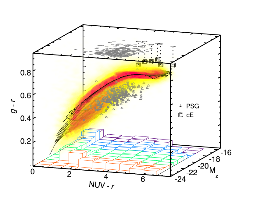
Figure 2: The 3-dimensional distribution of galaxies in the ($NUV-r$, $M_{z}$, $g-r$) space. The 3D plot presents the density distribution of 225 000 galaxies in the colour–colour–magnitude space with the increasing density going from yellow to red, the best-fitting polynomial surface as a mesh grid immersed in it, and standard deviations of the fitting residuals shown as bars in the ($NUV-r$, $M_{z}$) plane with their colours corresponding to the magnitude ranges in Fig. 1. PSGs (Goto, 2007), and compact elliptical galaxies (cE) are shown as tetrahedra and cubes. The top face of the plot demonstrates their projected positions on-to the ($NUV-r$, $M_{z}$) plane.

3.1 Connection to morphology

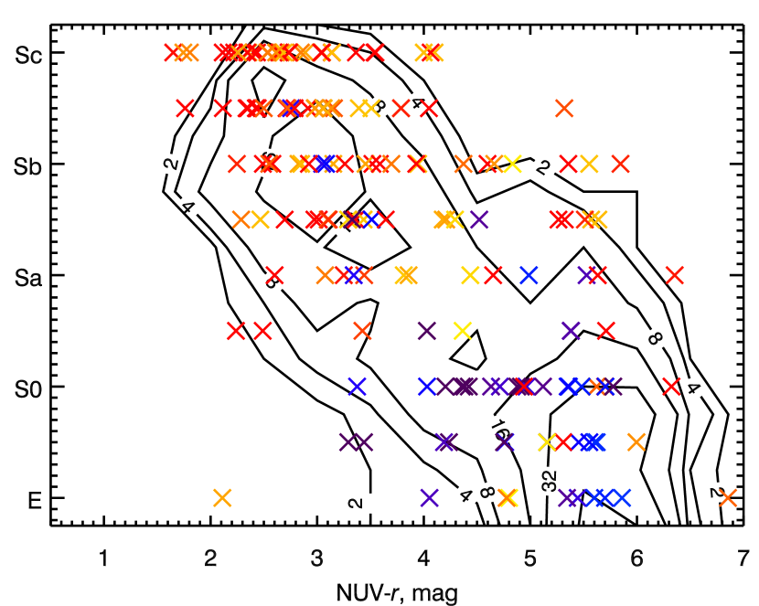
Figure 3: Connection between visually determined galaxy morphology (Fukugita et al., 2007) and a $NUV-r$ colour. Black contours correspond to galaxies following the relation (numbers are for the counts), while individual outliers beyond $1\sigma$ are shown as crosses with the colours representative of the deviation from the relation in the $g-r$ colour: yellow to red for galaxies above the relation, blue to violet for objects below it.

To explore the connection of the colour–colour–magnitude relation to galaxy morphology, we employed the morphological catalogue of SDSS galaxies (Fukugita et al., 2007) available through the Vizier service, which contains morphological types for 1 465 intermediate luminosity and giant galaxies at $Z>0.03$ from our sample. We see a continuous change of morphological types along the surface in the $NUV-r$ direction with a typical dispersion of 0.7$\dots$0.8 Hubble type. At the same time, the optical $g-r$ colour turns to be a very bad morphological indicator: the red sequence region contains galaxies of all morphologies from ellipticals to $Sc$ late-type spirals.

The two-dimensional histogram of morphologies vs $NUV-r$ colours is displayed in Fig. 3. One can see that the S0a and Sa galaxy types span a very broad range of colours demonstrating the difficulties of the visual classification of early-type disc galaxies. It corresponds to a simple linear correlation between the $NUV-r$ and a Hubble type which can be expressed as:

$$\mbox{TYPE}=6.6-1.1\cdot(NUV-r),$$

where the “TYPE” values will correspond to the Hubble types as $<0$ for E, 1 for S0, 2 for Sa, 3 for Sb, 4 for Sc, higher values for Irr. Red outliers ($NUV-r\mathrel{\hbox{\hbox to0.0pt{\hbox{\lower 4.0pt\hbox{$\sim$}}\hss}\hbox{$>$}}}4$ mag) above the surface (yellow and red points in Fig. 3) mostly have later types, i.e. spiral galaxies, while outliers below it (blue and violet points in Fig. 3) have earlier types compared to galaxies on the sequence with similar $NUV-r$ colours.

The connection between the morphology and the luminosity suggesting that more luminous galaxies have earlier morphological types is much looser and may be affected by the selection effects in our sample.

3.2 Outliers from the relation

We identify several classes of outliers from the relation comprising $\sim$2 per cent of the total sample (see Fig. 1, 2).

1. Early-type PSGs selected from the catalogue of H$\delta$-strong galaxies (Goto, 2007) (359 matches with our sample) populate a region $\sim$0.15 mag below the surface in $g-r$ spanning $3\mathrel{\hbox{\hbox to0.0pt{\hbox{\lower 4.0pt\hbox{$\sim$}}\hss}\hbox{$<$}}}NUV-r\mathrel{\hbox{\hbox to0.0pt{\hbox{\lower 4.0pt\hbox{$\sim$}}\hss}\hbox{$<$}}}5$ mag colours explaining the nature of “blue early-type outliers” from the morphology–$(NUV-r)$ relation described above. These are galaxies with truncated or multi-modal SFH where the last strong star formation episode has just been finished. The passively evolving newly formed stellar population reddens much faster in the $NUV-r$ colour than in the $g-r$ one so that a PSG at first departs from the blue part of the relation (right in Fig. 1) and notably later (after 2.5–3 Gyr) moves up increasing $g-r$ towards the locus of red sequence galaxies.

2. Compact elliptical galaxies (Chilingarian et al., 2009a; Price et al., 2009) are residing above the red sequence region of the colour–colour–magnitude relation at the low luminosity part. A few examples of new cE galaxies are shown in Fig 2. However, their colours are never redder than those of the most massive galaxies at the bright red sequence end. This fact is explained by their formation via severe tidal stripping of more massive progenitors, most likely early-type disc galaxies, by massive elliptical or cluster/group dominant galaxies. Progenitors of cEs are stripped in the innermost regions of galaxy clusters, when the SF is ceased because their interstellar medium is already removed by the ram pressure stripping created by the hot intergalactic gas (Gunn & Gott, 1972). Depending on the previous SFH, these objects must reside either on the colour–colour–magnitude relation, or slightly below it, in the PSG locus. During the relatively fast tidal stripping process lasting about 1 Gyr (Chilingarian et al., 2009a), their stellar population properties and colours change insignificantly while the mass and, consequently, the luminosity may decrease by a factor of 10 or more, hence moving a galaxy off the relation if it was sitting on it. Thus, red cE colours are explained by high stellar metallicities inherited from their progenitors which is confirmed by detailed studies of nearby cEs (Rose et al., 2005; Chilingarian & Bergond, 2010). There may be some very rare intermediate-age cEs originating from PSGs whose colours will be bluer, however their passive evolution will quickly move them above the colour–colour–magnitude relation.

3. Dusty starforming galaxies such as edge-on spirals are sometimes found above the flattened red part of the relation ($NUV-r\mathrel{\hbox{\hbox to0.0pt{\hbox{\lower 4.0pt\hbox{$\sim$}}\hss}\hbox{$>$}}}4$ mag) also being consistent with the locus of late-type morphological outliers. Their positions are explained by the extinction vector direction shown in Fig. 1. If internal extinction is very strong then a galaxy is moved up-right in the diagram and may end up above the locus of red sequence galaxies.

4. Galaxies with strong ongoing SF but yet small mass fractions of newly formed stars including ongoing and recent mergers may have very peculiar colours because of strong nebular emission lines and/or large quantities of dust.

5. Narrow-line AGNs having low contribution of their nuclei to the total light in the optical band and hence classified as normal galaxies by the SDSS pipeline may have strong UV excess. We did not apply any particular filtering to our data to exclude these objects, therefore our sample may be slightly contaminated by them at a sub-per cent level.

6. “Non-physical” objects: galaxies casually overlapping with either foreground stars or galaxies at different redshifts create outliers which may be located in almost any part of the parameter space except the region very red in ($NUV-r$) and very blue in ($g-r$).

4 Discussion

4.1 Effects of stellar population evolution and internal extinction

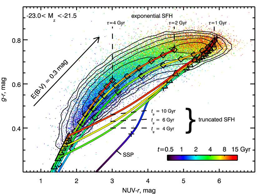
Figure 4: Connection between galaxy positions on the colour–colour–magnitude relation and their SSP-equivalent stellar populations. The slice of the relation in a narrow luminosity range ($-23<M_{z}<-21.5$ mag) is displayed in the colour–colour projection. Mean ages of stellar populations of 40,000 galaxies obtained from the fitting of their SDSS DR7 optical spectra are colour–coded. The evolutionary tracks of stellar population models without internal extinction for the solar metallicity and various SFH are overplotted (see text). The colours of the tracks correspond to the ages of synthetic galaxies formed 12 Gyr ago, the ticks on the tracks are given every 1 Gyr. The $NUV-r$ colours in the models are empirically corrected by $-0.7$ mag (see the text).

The distribution of galaxies in the colour–colour–magnitude space is governed by three factors: (1) stellar mass, (2) star formation and chemical enrichment histories including the ongoing SF, and (3) internal extinction. Therefore, there must be a connection between galaxy positions on the diagram and their stellar population properties. We fitted a sub-sample of 133 000 SDSS DR7 spectra with simple stellar population (SSP) models using the nbursts technique (Chilingarian et al., 2007b, a) and hence obtained their SSP-equivalent ages and metallicities. The nbursts technique includes the multiplicative polynomial continuum that absorbs flux calibration errors and makes the fitting insensitive to the internal extinction in a galaxy. We also notice that SDSS spectra obtained in 3 arcsec wide circular apertures may not be representative of entire galaxies in case of strongly extended objects with notable gradients of the stellar population properties. However, we can draw some qualitative conclusions.

Even in the over-simplified case of SSP-equivalent parameters, we observe a strong connection between average stellar population properties of galaxies and their position in the ($M_{z},NUV-r,g-r$) parameter space. Galaxies sitting close to the best-fitting surface exhibit moderate metallicity gradient as a function of luminosity and almost no variations in the colour–colour plane except the blue end of the sequence ($NUV-r\mathrel{\hbox{\hbox to0.0pt{\hbox{\lower 4.0pt\hbox{$\sim$}}\hss}\hbox{$<$}}}2.5;g-r\mathrel{\hbox{\hbox to0.0pt{\hbox{\lower 4.0pt\hbox{$\sim$}}\hss}\hbox{$<$}}}0.5$) where the metallicity quickly decreases. The luminosity–metallicity relation of early-type galaxies known to be responsible for the tilt of their optical colour–magnitude relation (Kodama & Arimoto, 1997) similarly causes the tilt of the colour–colour–magnitude surface in its red part.

The observed age effects in the colour–colour projection are more important. At intermediate and high luminosities, the age smoothly increases along the sequence from $\sim$500 Myr at $NUV-r\approx 1.5,g-r\approx 0.3$ to 13 Gyr at the red end. For low luminosity galaxies, the oldest SSP-equivalent ages of red galaxies decrease to 10 Gyr at $M_{z}=-18$ mag being in accordance with the known anti-correlation of mean stellar population ages with luminosities of dwarf elliptical galaxies in clusters (van Zee et al., 2004; Michielsen et al., 2008; Chilingarian et al., 2008; Chilingarian, 2009; Smith et al., 2009a, b). Because of the same effect, the upper “edge” of the broad red sequence in the ($NUV-r;M_{z}$) CMD is strongly tilted at $M_{z}>-19$ mag.

At all luminosities, there is a notable age gradient across the sequence, that is, higher $g-r$ colours correspond to older populations. Also, the dispersion of age estimates ($\log t$) increases while moving towards blue colours with values totally uncorrelated with colours at the very blue end of the sequence corresponding to mean stellar ages $t\mathrel{\hbox{\hbox to0.0pt{\hbox{\lower 4.0pt\hbox{$\sim$}}\hss}\hbox{$<$}}}500$ Myr.

In Fig. 4 we present a luminosity slice ($-23.0<M_{z}<-21.5$ mag) of the sample having the median SSP-equivalent metallicity $[$Fe/H$]=-0.02$ dex ($\langle[$Fe/H$]\rangle=0.13$ dex) and the median redshift $Z=0.11$ ($\langle Z\rangle=0.03$) corresponding to the light travel time of $\sim 1.4$ Gyr. At this redshift range, the 3 arcsec wide apertures enclose a large fraction of light from galaxies. The qualitative behaviour of mean stellar population ages at other luminosities is similar.

We also present the evolutionary tracks for galaxies having various SFH types. The models were constructed from the pegase.2 (Fioc & Rocca-Volmerange, 1997) models computed using the synthetic low-resolution BaSeL stellar library (Lejeune et al., 1997) for $NUV-r$ colours, and $g-r$ colours predicted by another family of stellar population models (Vazdekis et al., 2010) computed using a large Medium-resolution Isaac Newton Telescope library of empirical spectra (MILES, Sánchez-Blázquez et al., 2006). The combination of the two families of stellar population models was essential, as Maraston et al. (2009) demonstrated that the offsets between predicted and observed colours of red galaxies in the SDSS photometric system was due to the nature of synthetic stellar spectra used to construct stellar population models. The proposed solution was to use models based on empirical stellar spectra. The MILES stellar library used to construct models presented here, has the best coverage of the stellar atmosphere parameters compared to all other existing published sources except the high-resolution ELODIE library which, however, has too narrow wavelength coverage making the computation of $g$ and $r$ colours impossible. The $NUV-r$ colours for all models displayed in Fig. 4 were empirically corrected by $-0.7$ mag. This offset is probably of the same nature as that described by Maraston et al. (2009), however no models based on empirical stellar spectra are available in the NUV yet.

The tracks shown in Fig. 4 were computed as follows. First, we computed colours and luminosities of simple stellar populations having $[$Fe/H$]=$0 dex using the pegase.2 code for the ages of 30, 50, 100 Myr and further till 17 Gyr with a step of 50 Myr. Second, we computed $g-r$ colours from the MILES-based models and interpolated them to the same age grid. The resulting SSP track is shown in Fig. 4 – its young part is strongly offset from the observed distribution of galaxies towards red $NUV-r$ then joining the main red sequence concentration at ages $t>5$ Gyr. Third, we integrated the computed SSP luminosities in different photometric bands up-to 12 Gyr using two families of an SFH: (a) exponentially declining star formation rate (SFR) with the three characteristic timescales $t_{\mbox{exp}}=1,2,4$ Gyr; and (b) truncated SFHs: constant SFR until a given moment of time from the galaxy formation epoch ($t_{\mbox{tr}}=4,6,10$ Gyr) followed by the immediate SF cessation and passive evolution afterwards.

Our galaxy evolutionary tracks are simpler than real galaxies because they do not include the intrinsic metallicity evolution and other processes such as gas infall from filaments or satellites, mergers, etc., however, we can use them for some qualitative conclusions:

1. SSP models at low and intermediate ages ($t<5$ Gyr) to not have any corresponding galaxies observed that suggests that (obviously) none of the massive galaxies in our sample was formed recently and quickly. However, it matches quite well the locus of the oldest red sequence galaxies.

2. The main colour sequence can be explained by galaxies formed immediately after the Big Bang (about 12 Gyr taking into account the median redshift of our sample) and having various types of a SFH. In its main part, the slope of the colour–colour relation and the direction of the internal extinction match each other very well.

3. A galaxy having a constant SFR will end up near the low blue end of the sequence and can be moved up–right along it by the internal extinction. A family of exponentially declining SFH with different characteristic timescales form a curved sequence well corresponding to the observed relation. The $NUV-r$ colour evolution pace at $3<NUV-r<5$ mag anticorrelates with the SFR characteristic timescale (see also Wyder et al. (2007) for a similar plot in the ($NUV-r,u-r$) colour space without any selection on the luminosity). Models for lower metallicities well reproduce the colour–colour relation at lower luminosities suggesting the universality of exponentially declining SFHs. We stress that this SFH type is not the only one that is able to explain the observed galaxy distribution in the colour–colour–magnitude space, however, it is the simplest model with the smallest number of free parameters compared to other alternatives (e.g. multiple starbursts, an exponentially declined law with an additional burst).

4. Galaxies having truncated SFHs have a very short transition phase on their way to the red sequence region lasting about $1$ Gyr after the SF cessation when their $NUV-r$ colour reddens radically, by $\sim 3$ mag while the $g-r$ change remains about 0.2 mag. The PSG locus below the main colour sequence is well matched by this transition phase and their rareness is consistent with a short duration of the transition.

5. Dusty star-forming galaxies above the sequence at red $NUV-r$ colours are also explained: they are moved up–right from the sequence following the direction of the extinction vector.

6. The shapes of evolutionary tracks for galaxies with exponentially declining SFH clearly shows that the evolution of a majority of galaxies goes along the relation during 6–8 Gyr. Therefore, we would expect a weak evolution of the presented colour–colour–magnitude relation shape at least up-to a redshift $Z\sim 0.9$, although the distribution of galaxies on it will evolve. This suggests it to be a unique search instrument for distant galaxy clusters using broad band $giJ$ images.

4.2 Colour–colour–magnitude relations in other colour pairs

We found similar photometric relations in other colour pairs, however they are more strongly affected by observational biases and galaxy evolutionary phenomena. Colour–colour–magnitude relations involving only optical colours are very tight because of strong degeneracies between the colours but for the same reason have very limited astrophysical applications. For example, in the ($u-r,g-r,M_{r}$) colour space the $u-r$ is close to $\sim 2\times(g-r)$ at all luminosities, i.e. they are linearly dependent for most galaxies, hence virtually no information is added by the third dimension.

4.2.1 Other near-UV–optical colour combinations

The colour–colour–magnitude relation remains in place when other optical colour combinations together with the $NUV$ are used provided that there is enough wavelength lever in the optical colour to distinguish between red and blue galaxies. That is, colours like $u-r$, $g-i$, $g-z$, $r-z$ but not $r-i$ and $i-z$. In Appendix C we provide figures similar to Fig. 1 constructed for different colour pairs.

Photometric measurements in the $u$ band have relatively poor quality compared to $g$ and $r$, therefore the residuals of the $(NUV-r,u-r,M_{r})$ relation are about four times larger than those of $(NUV-r,g-r,M_{r})$. An additional factor increasing the scatter is an important difference between the extinction vector direction and the blue slope of the relation in the ($NUV-r,u-r$) plane compared to ($NUV-r,g-r$) increasing the scatter at $NUV-r<4$ mag.

The $(NUV-i,g-i,M_{i})$ relation has fitting residuals about 50 per cent higher than the $(NUV-r,g-r,M_{r})$ one, although one would expect them to be similar given very high quality of $i$ and $r$ band photometry and similar dependence of these colours on the stellar population evolution. We explain this by higher uncertainties of the $k$-correction computation in the $i$ band connected to a broad range of the H$\alpha+[$Nii$]$ emission line strength in our galaxies. In our sample, except the very low-redshift objects ($Z<0.03$), the observed-frame $i$ band may be contaminated by the H$\alpha+[$Nii$]$ emission in a galaxy which may vary a lot from object to object. However, during the $k$-correction computation we rely on some average line strength provided by the template spectra of Blanton & Roweis (2007). Therefore, objects with very weak or very strong emission lines will have their observed $r-i$ colours redder or bluer than what is predicted by the templates and what was included in the 2D-polynomial approximations of $k$-corrections. Hence, the $i$ band $k$-correction values may be biased. Even though, given a $\sim$50 per cent larger range of $g-i$ colours compared to $g-r$, the relation in this colour space may be used in the same way as the one presented in Section 3.

The ($NUV-z$, $g-z$) colour combination provides another very good alternative to $(NUV-r,g-r,M_{r})$, however with $\sim$80 per cent larger scatter because of lower photometric quality in the $z$ band compared to $r$ in the SDSS. The remarkable features of this relation are: (a) a notably higher luminosity tilt in the red sequence region and (b) low residuals in the blue part of the relation caused by even better coincidence of the colour change direction due to the stellar population evolution and internal extinction than in the ($NUV-r$, $g-r$) plane.

The ($NUV-z$, $r-z$) colour pair starts to suffer from very similar behaviour of $r$ and $z$ burdened by relatively high photometric errors in the $z$ band. Therefore, although the $r-z$ colour range is nearly the same as that in $g-r$, the dispersion of the residuals is notably higher that complicates the usage of the ($NUV-z$, $r-z$, $M_{z}$) colour–colour–magnitude relation.

4.2.2 Combinations including Far-UV and NIR colours

GALEX $FUV$ measurements have on average much worse quality than the $NUV$ ones because of the lower detector sensitivity and also lower fluxes for intermediate-age and old galaxies. However, we still can see similar colour–colour–magnitude relations if we use $FUV$ magnitudes instead of $NUV$ although with higher residuals especially in the low-luminosity part of the relation where the mean surface brightness of galaxies decreases. The computed $k$-corrections also have higher uncertainties in $FUV$ as well as internal extinction effects introducing additional scatter.

The red sequence region in the colour–colour projection extends from $\sim$2.5 mag in $NUV-r$ to $\sim$4 mag in $FUV-r$ due to even higher sensitivity of $FUV$ colours to small fractions of young stars. However, all combinations involving $FUV$ magnitudes are sensitive to the UV upturn in old early-type galaxies (Code, 1969; Bertola et al., 1982) likely caused by the stellar evolution (Yi et al., 1997), which results in the ambiguity of the relation in the red sequence region. That is, after some “turning point” (7–8 Gyr), the $FUV-r$ colour becomes bluer when the stars are getting older.

We used NIR UKIDSS photometry to test the existence of photometric relations in the combinations involving optical-NIR colours. None of the combinations except ($NUV-Y$, $g-Y$, $M_{Y}$) provides a relation having similar tightness to what we detected in the optical colours: the fitting residuals are of an order of 0.2 mag or larger.

It is known (see e.g. Maraston, 2005) that $JHK$ colours are sensitive to AGB stars presenting in intermediate-age stellar populations, and that at certain ages (1–2 Gyr) the optical–NIR colours ($g-H$ or $r-H$) are dominated by them being redder than the colours of old stellar populations by a few tenths of a magnitude. Then, given a much larger range of e.g. $NUV-H$ than that of $r-H$, this excess will be significant, and it will strongly depend on the SFH of a given galaxy, so that galaxies with intermediate $NUV-H$ colours having different SFH families may have significantly different $g-H$ or $r-H$ colours smearing out the intermediate-to-red part of the relation except its very red end. In addition, optical-NIR colours are more sensitive to the metallicity than the optical ones. Hence, the natural relatively low metallicity spread of galaxies at a given luminosity will introduce high scatter of their $g-H$ or $r-H$ colours. Because of the AGB phase, for truncated SFHs, the colour evolution in the ($NUV-H$, $g-H$) plane will also be more complex than in the optical colour and it will strongly depend on the truncation time.

4.3 Redshifts from three photometric points

This section of the paper aims at an independent mathematical proof of the existence of the tight UV–optical colour–colour–magnitude relation of galaxies. The detailed discussion of the technique and its practial applications to the existing photometric survey data will be provided in a separate paper.

The mathematical consequence of the relation and smooth dependencies of $k$-corrections on observed colours is the possibility of the existence of a univocal functional dependence of a redshift on observed colours and magnitudes of galaxies. Such a dependence, if found, would confirm the existence of the universal colour–colour–magnitude relation. Importantly, it arises from a non-zero curvature of the colour–colour–magnitude surface and significantly different colour–magnitude distributions for the two colours used. In a degenerated case, e.g. $(u-r,g-r,M_{r})$ where the two colour–magnitude distributions are very close to the linear dependence and, therefore, galaxies reside on a surface very similar to a plane, the photometric redshift determination becomes impossible.

For the following computations we define the two subsamples from the main galaxy sample extended to the redshift $z=0.52$ (270 016 objects) by using their $k$-corrected $g-r$ colours, red galaxies ($g-r>$0.73 mag, 77 070 objects) and blue galaxies ($g-r<$0.7 mag, 167 157 objects) excluding a small fraction of objects in the “green valley”. These samples were again separated into a low- ($z\leq 0.25$) and high-redshift ($z>0.25$) parts containing 214 770 (32 317 red $+$ 160 310 blue) and 56 275 (45 365 red $+$ 7 227 blue) galaxies correspondingly. Here, most of blue galaxies in the high-redshift sample come from the deep SDSS Stripe 82 imaging (Adelman-McCarthy et al., 2006) and the fraction between blue and red galaxies clearly demonstrates the target selection algorithm of SDSS biased towards luminous red galaxies at intermediate and high redshifts.

We approximated the spectroscopic redshifts of galaxies in our low-redshift subsample as a three-dimensional polynomial function of observed $r$, $NUV-r$, and $g-r$, and attempted to recover the photometric redshifts $z_{\mbox{phot}}$ (Fig 5). The dispersion $\sigma(\Delta(z))$ of the residuals $\Delta(z)=(z_{\mbox{phot}}-z_{\mbox{spec}})/(1+z_{\mbox{spec}})$ of 0.025 together with catastrophic failure rate (defined as fraction of objects with $\Delta(z)>3\sigma(\Delta(z))$) of $\eta=0.8$ per cent is comparable to the best available photometric redshift techniques exploiting multi-band FUV-to-NIR photometry, sophisticated mathematical and statistical algorithms (Way & Srivastava, 2006) and additional morphological information (Wray & Gunn, 2008). For red and blue galaxies, the residuals and the catastrophic failure rates were: $\sigma(\Delta(z))_{\rm{red}}=0.021$, $\eta_{\rm{red}}=2.2$ per cent and $\sigma(\Delta(z))_{\rm{blue}}=0.024$, $\eta_{\rm{blue}}=0.7$ per cent.

Consequently, at higher redshifts when the restframe $NUV$ photometric band shifts to the optical domain, it should be possible to determine photometric redshifts precisely using $u-r-z$, $g-r-z$, or $g-i-Y$ broadband photometry. We tested this hypothesis with our high-redshift subsample by fitting their redshifts as a function of observed SDSS ($z$, $u-z$, $r-z$) and obtained the residuals having a dispersion $\sigma(\Delta(z))=0.036$ and the rate of catastrophic failures $\eta=1.1$ per cent. For red and blue galaxies, the residuals and the catastrophic failure rates were: $\sigma(\Delta(z))_{\rm{red}}=0.034$, $\eta_{\rm{red}}=1.0$ per cent and $\sigma(\Delta(z))_{\rm{blue}}=0.047$, $\eta_{\rm{blue}}=1.2$ per cent. These relatively large errors are mostly due to the very poor quality of $u$-band Petrosian magnitudes having typical uncertainties of an order of 0.3 mag for high-redshift galaxies. We notice here, that if one uses model magnitudes instead of Petrosian ones, the relation becomes much tighter for the red subsample ($\sigma(\Delta(z))_{\rm{red}}=0.027$), however it nearly disappears for blue galaxies whose $u$-band model magnitudes do not correspond to their real photometric properties because of light distributions being very far from regular exponential or de Vaucouleurs profiles.

The demonstrated possibility of the precise photometric redshift computation for both, red and blue galaxies with a small fraction of outliers from three photometric points involving a near-UV and optical colours proves the existence of the tight unversal colour–colour–magnitude relation for normal galaxies of all types, not only red sequence objects.

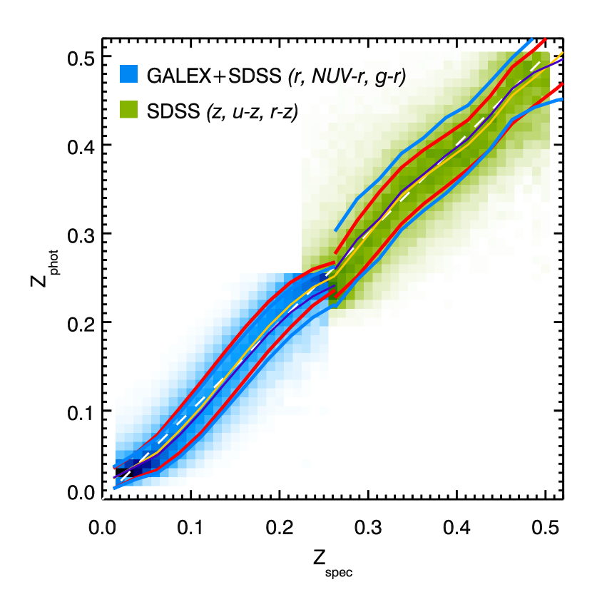
Figure 5: Recovery of galaxy distances from three photometric points. Density histograms of photometric redshift ($Z_{\mbox{phot}}$) determination by fitting their spectroscopic redshifts ($Z_{\mbox{spec}}$) as a polynomial function of three parameters: an observed magnitude and two observed colours corrected for the Galactic extinction. The blue plot displays a sample of 214 000 low-redshift galaxies ($0.03<Z<0.25$) with NUV, $g$, and $r$ photometric measurements from GALEX and SDSS. The green plot is sample of 56 000 intermediate-redshift galaxies ($0.2<Z<0.52$) whose redshifts $Z_{\mbox{phot}}$ were determined using $u$, $r$, and $z$ SDSS DR7 photometric data. Red and blue solid lines denote median of $Z_{\mbox{phot}}$ and the standard deviations of $(Z_{\mbox{phot}}-Z_{\mbox{spec}})/(1+Z_{\mbox{spec}})$ residuals for blue and red galaxy subsamples respectively.

We compare these metrics to the existing photometric redshifts techniques. Using the “le phare” photometric redshift code combined with a template optimisation procedure and the application of a Bayesian approach, based on the sample of galaxies with 9 individual photometric measurements of a quality similar to ours, Ilbert et al. (2006) find the dispersion $\sigma(\Delta(z))$ to be 0.025 and $\eta=1.9$ per cent (though we stress that the authors defined the catastrophic failure limit at the fixed level of 0.15 which corresponded to $6\sigma$ in their statistics). Mobasher et al. (2007) analyse the performance of different photometric redshift codes on a dataset that comprises 16 photometric points for every SED in question. The best result achieved in their study with own method reaches the dispersion of residuals as low as $\sigma(\Delta(z))=0.033$ and $\eta=2.2$ per cent. The SDSS database provides several photometric redshift estimates obtained as described in Adelman-McCarthy et al. (2007). We have extracted three of them: (1) those obtained from the comparison of the observed colors of galaxies to a semi-empirical reference set (hereafter photoz) from the photoz table, and (2) neural network estimators derived from galaxy magnitudes (“D1”) and (3) colours (“CC2”) from the photoz2 table. In general, they perform quite well for red galaxies in our high-redshift subsample ($\sigma(\Delta(z))_{\rm red,photoz}=0.020$ and $\eta_{\rm red,photoz}=1.7$ per cent, $\sigma(\Delta(z))_{\rm red,D1}=0.020$ and $\eta_{\rm red,D1}=1.6$ per cent, $\sigma(\Delta(z))_{\rm red,CC2}=0.023$ and $\eta_{\rm red,CC2}=1.7$ per cent). However, similarly to our approach, the quality is worse for blue galaxies: $\sigma(\Delta(z))_{\rm blue,photoz}=0.042$ and $\eta_{\rm blue,photoz}=3.4$ per cent, $\sigma(\Delta(z))_{\rm blue,D1}=0.039$ and $\eta_{\rm blue,D1}=2.0$ per cent, $\sigma(\Delta(z))_{\rm blue,CC2}=0.044$ and $\eta_{\rm CC2}=1.7$ per cent. One has to keep in mind that (1) these techinques use a lot of additional information (e.g. morphology, size, etc.) and (2) all the galaxies in the spectroscopic SDSS sample in fact constitute a training sample of these methods, so one has to check those numbers against massive third-party redshift surveys.

We also note that since the redshift determination by three photometric points is a mere mathematical consequence from the colour-colour-magnitude relation, photometric redshift outliers are themselves objects that fall aside from the relation, namely PSGs, dusty starbursts, and AGN.

To summarise, compared to existing photometric redshift techniques, presented method requires a factor of 3 to 5 more modest investment in observing time (due to the fact that individual galaxy measurements do not need to be made in as many photometric bands), being able to provide redshifts for large samples of galaxies at the same or better level of accuracy. Moreover, proposed polynomial evaluation is significantly simpler from the methodological point of view than $\chi^{2}$ minimization with Bayesian priors used in mainstream photometric redshift codes.

There are two main disadvantages of our approach: (1) it is not precise for non-typical galaxies, i.e. outliers from the colour–colour–magnitude relation; (2) it works only for those regions of the parameter space, that are well sampled with spectral redshift measurements. Latter means e. g. that it is possible to go beyond the SDSS spectral sample magnitude limit retaining the declared precision of our method if one uses an external source of spectral redshifts to calibrate the functional relation to work with the SDSS photometry at fainter magnitudes. But without such a calibration, photometric redshifts estimates for faint galaxies will be wrong.

Conceptually, the presented multi-dimensional polynomial fit resembles the training of artificial neural networks sometimes used for the photometric redshift determination (e.g. D’Abrusco et al., 2007), though the underlying machinery is different. In both cases, there is a non-linear transformation (a 3D-polynomial function in our case or consequent multi-level sigmoid transformations in case of neural networks) of some input measurements into the output redshift estimate. And the coefficients of a transformation are tuned (“trained”) in a way to work as good as possible for the reference (“training”) dataset. Hence, both methods unlike $\chi^{2}$ template fitting family are insensitive to systematic errors of the input data. That is, the “templates” are constructed from the dataset itself and are tolerant to its problems by construction.

5 Summary

We presented the universal very tight colour–colour–magnitude relation in optical and near-UV filters followed by the vast majority of non-active galaxies of all morphological types covering at least 8 magnitudes in luminosity from the sample including 225 000 low-redshift ($Z<0.27$) galaxies observed by SDSS and GALEX surveys. A special case is the connection of the optical $g-r$ colour to the $NUV-r$ colour and $M_{r}$ luminosity which we approximated by a low-order polynomial surface with the residuals of $\sim$0.03–0.07 mag in the entire covered luminosity ($-23.5<M_{r}<-15.5$ mag) and colour ($0<NUV-r<7.5$ mag) ranges.

We have demonstrated that there is a strong correlation between the $NUV-r$ colour and the galaxy morphology while for the optical $g-r$ colour this correlation is much weaker. We identified several classes of the outliers constituting about 2 per cent of the total galaxy population and explained their nature, the most important being rare compact elliptical and poststarburst E+A galaxies.

We have performed stellar population modelling and shown that the relation can be explained by galaxies having constant and exponentially declining SFHs, while truncated SFHs with very rapid colour evolution after the SF cessation explain the properties of E+A outliers. The most important conclusion is the predicted weak dependence of the colour–colour–magnitude relation shape on a redshift up-to $Z\sim 0.9$ that will allow to use it for search of distant galaxy clusters in 3-colour broad band images.

The existence of such a tight photometric relation suggests the possibility of the high-precision photometric redshift estimates using only three photometric points that we have also illustrated. Our empirical photometric redshift technique using a minimalistic input dataset has a quality comparable to or better than most published $Z_{\mbox{phot}}$ techniques, while it is much simpler to implement.

The detailed astrophysical interpretation of the described photometric relation still has to be done. However, it can be used already as a powerful galaxy classification and selection instrument based only on their integrated photometry as well as a tool to search for representatives of rare galaxy types in photometric galaxy samples.

Appendix A Validation of the result

Two factors may in principle lead to the spurious creation of the colour–colour–magnitude relation presented in this work: (a) sample selection biased toward specific colours corresponding to the described surface, (b) serious faults in the $k$-correction computation artificially bringing most galaxies to that relation.

As far as we apply no selection to the SDSS DR7 spectroscopic sample of galaxies based on their morphology, colours, sizes etc., and GALEX is a full-sky survey providing photometric information for all detected objects, the only source of selection effects may be the spectroscopic target selection of SDSS. The corresponding algorithms are exhaustively described (Eisenstein et al., 2001; Strauss et al., 2002), and we find no evidences for them to introduce any biases on galaxy selection that may lead to the creation of “empty” regions in the colour–colour–magnitude parameter space. This is also well illustrated by the broad and very well filled colour distribution of SDSS galaxies (Strateva et al., 2001; Blanton et al., 2003a; Baldry et al., 2004) and studies of galaxy luminosity functions based on SDSS (Blanton et al., 2003b).

In order to test the existence of potential problems in the $k$-correction computations, we have conducted two specific tests. For this, we selected two sub-samples of galaxies in narrow redshift ranges, $\Delta z_{1}$: $0.03<z_{1}<0.05$ (24 319 galaxies) and $\Delta z_{2}$: $0.08<z_{2}<0.10$ (37 303 galaxies). We chose relatively low-redshift samples because the SDSS targeting algorithm has a limiting magnitude $r=17.77$ mag in a 3 arcsec aperture so that galaxies at higher redshifts do not sample well the luminosity axis of the parameter space.

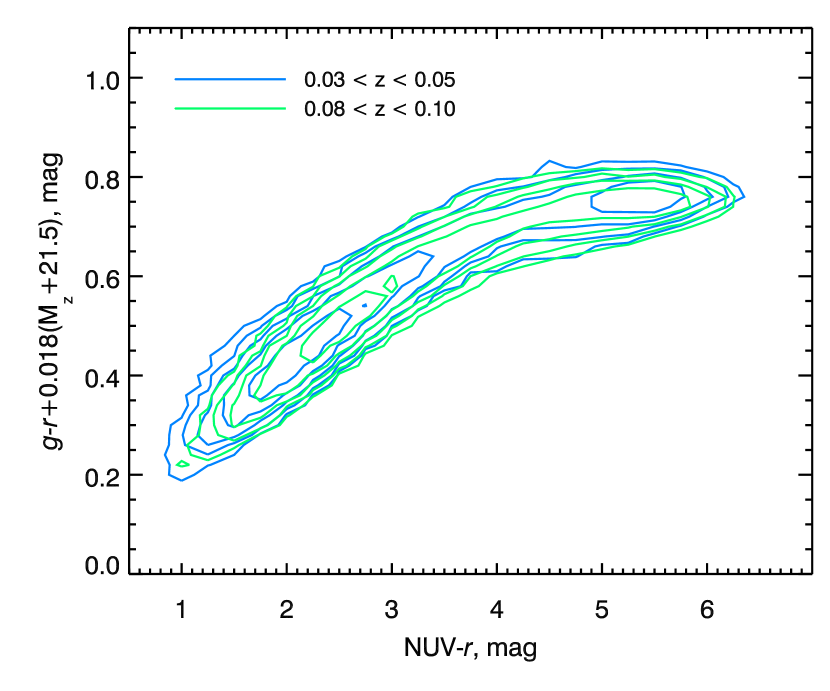
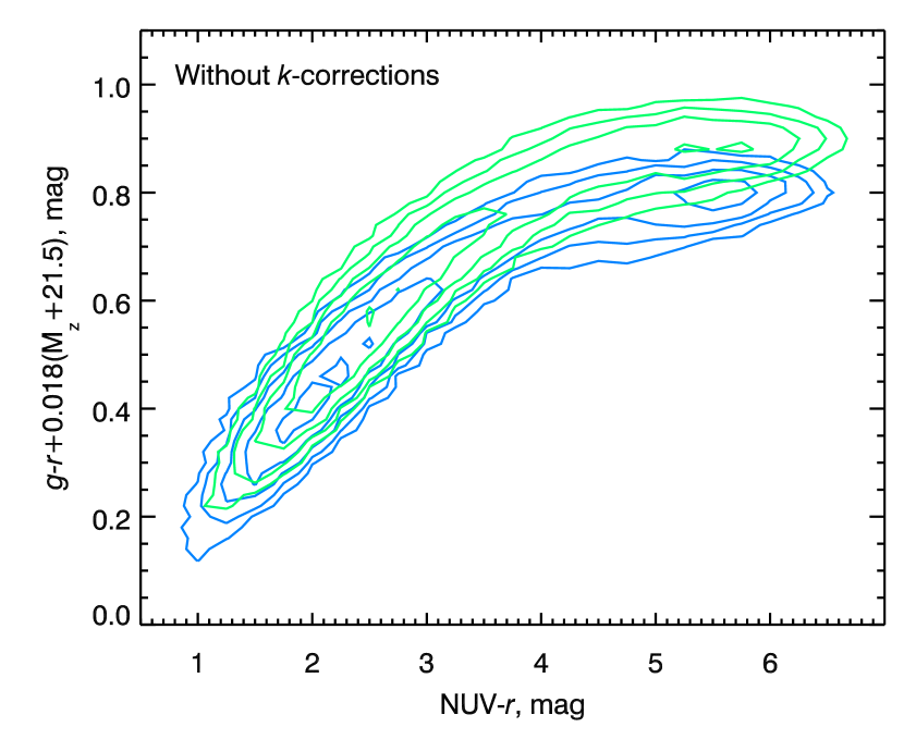
Figure 6: Tests with the two sub-samples of galaxies in narrow redshift ranges. The top panel demonstrates the number density plots for galaxies in two narrow redshift ranges in the projection shown in green and blue, corresponding to the edge-on view of the colour–colour–magnitude relation. The bottom panel is the same as the top one, but without applying $k$-corrections to the measurements.

The first test was to compare the colour–colour–magnitude distributions of galaxies in the two sub-samples. In case of $k$-correction computation problems, one would expect systematic differences between the two sub-samples, which we have not detected (see Fig. 6a for an “edge-on” view of the relation).

The second test was to entirely disable the $k$-correction computation for these two sub-samples. Because $k$-corrections do not change significantly within the narrow redshift sub-samples, but do change between the sub-samples, one would expect to get two tight colour–colour–magnitude sequences qualitatively resembling the relation for $k$-corrected magnitudes, but with some quantitative differences such as the blue cloud slopes and red sequence positions. We obtained the result exactly as predicted by this intuitive assumption. The edge-on views of the non $k$-corrected relations are presented in Fig. 6b.

However, the strongest argument supporting the existence of a universal colour–colour–magnitude relation in UV–optical colours is the possibility of computing photometric redshifts using only three observed colours as demonstrated in the Discussion section.

Appendix B Fitting surfaces into strongly non-uniform three-dimensional scattered datasets

A surface fitting procedure is an essential mathematical component required to obtain results presented in the paper. The observational photometric datasets for galaxies from wide-field survey have strongly non-uniform distribution in the colour–colour–magnitude space due to the superposition of the complex distribution of galaxies connected to their physics and various selection effects and observational biases.

Using visual inspection, we revealed a distribution of points in the colour–colour–magnitude space close to a smooth surface, but applying standard $\chi^{2}$-based linear surface fitting techniques did not yield the results of a reasonable quality because: (a) the density of points in the NUV-colour–magnitude plane varies by several orders of magnitude while the individual measurements have comparable quality; (b) distribution of points around the surface is sometimes significantly asymmetric and non-Gaussian. The former property of the distribution leads to the fact that the scarcely populated regions can deviate significantly from the surface without notable change of the goodness-of-fit as the best-fitting surface tries to minimize the deviation in the densest regions of the parameter space. The latter property leads to the biased fitting results as the $\chi^{2}$ technique assumes the Gaussian distribution. The $\kappa$-sigma clipping technique will not solve the problem here because we are dealing with a large number of points deviating from the symmetric distribution and not with individual outliers.

To tackle these issues in a simple way, we decided to use a two–step technique for the surface fitting. First, we defined a fine grid (cell size of about 0.25$\times$0.25 mag) in the NUV-colour–magnitude plane and in every bin computed median values of the optical colour being fitted. This allowed us to pick up the maxima of the (e.g. $g-r$) colour distributions in every bin and not the mean values, that was critical in order to account for the asymmetrical distribution of points around the surface. Then we filtered out the values where the 2D-histogram counts in a given bin were below some threshold (usually, 5 or 7 galaxies). At the second step, we fitted a low-order polynomial surface into these median values using a standard routine fitting linearly the polynomial coefficients and assigning equal weights to all points remained after the filtering at the first stage. This way we took into account the strongly non-uniform distribution of galaxies in the NUV-colour–magnitude plane.

This two–step approach resulted in almost flat distribution of residuals displayed in Fig. 1 and in the next Appendix.

Appendix C Colour–colour–magnitude relations in different colour combinations

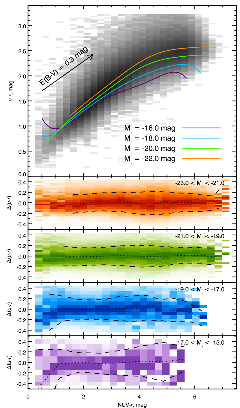
Figure 7: The same as Fig. 1 but for the ($NUV-r$, $u-r$, $M_{r}$) space.

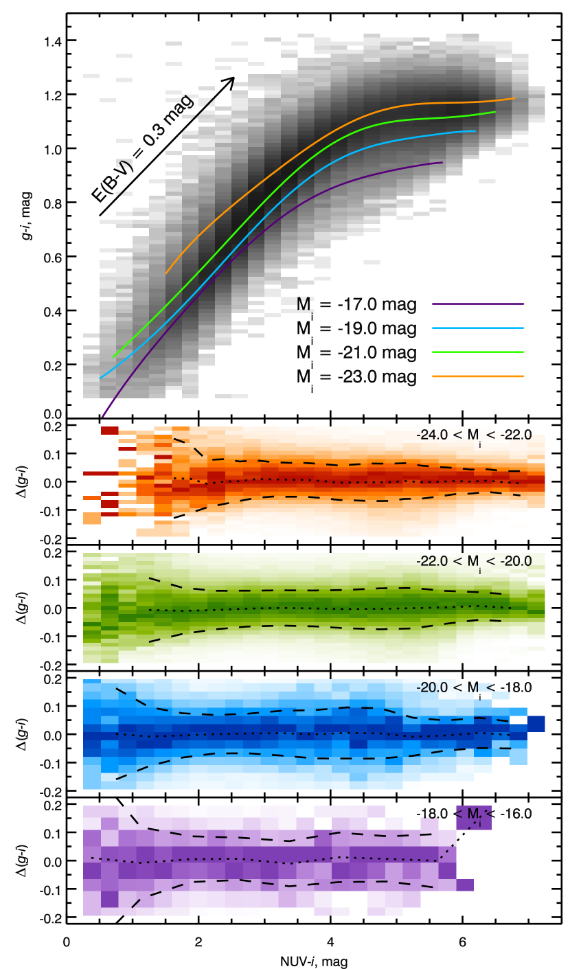
Figure 8: The same as Fig. 1 but for the ($NUV-i$, $g-i$, $M_{i}$) space.

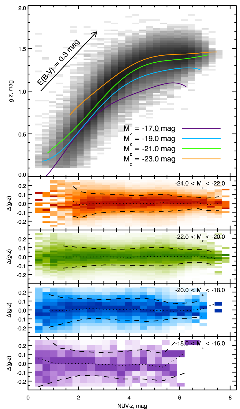
Figure 9: The same as Fig. 1 but for the ($NUV-g$, $g-z$, $M_{z}$) space.

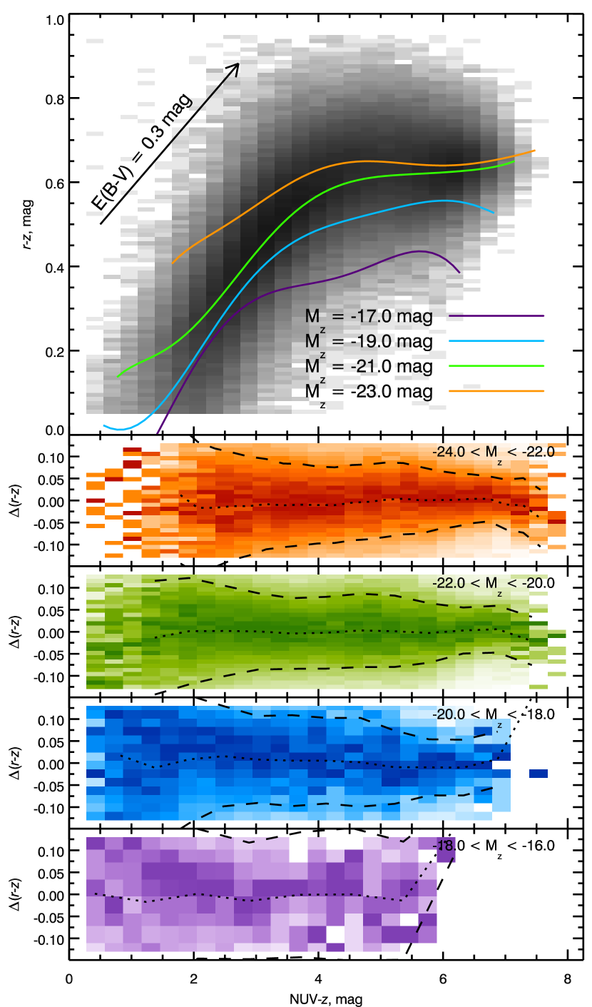
Figure 10: The same as Fig. 1 but for the ($NUV-z$, $r-z$, $M_{z}$) space.

In Fig. 7–10 we show the colour–colour projections of the colour–colour–magnitude relation in different near-UV–optical colours described in Section 4.2. All the fitting results including the coefficients of the best-fitting surfaces, fitting residuals in colour–magnitude bins and other essential information for the usage of the relations are provided in the electronic form.

References

- Abazajian et al. (2009) Abazajian, K. N., et al. 2009, ApJS, 182, 543
- Adelman-McCarthy et al. (2007) Adelman-McCarthy, J. K., et al. 2007, ApJS, 172, 634
- Adelman-McCarthy et al. (2006) Adelman-McCarthy, J. K., et al. 2006, ApJS, 162, 38
- Baldry et al. (2004) Baldry, I. K., Glazebrook, K., Brinkmann, J., Ivezić, Ž., Lupton, R. H., Nichol, R. C., & Szalay, A. S. 2004, ApJ, 600, 681
- Bertola et al. (1982) Bertola, F., Capaccioli, M., & Oke, J. B. 1982, ApJ, 254, 494
- Blanton et al. (2003a) Blanton, M. R., et al. 2003a, ApJ, 594, 186
- Blanton et al. (2003b) Blanton, M. R., et al. 2003b, ApJ, 592, 819
- Blanton & Roweis (2007) Blanton, M. R. & Roweis, S. 2007, AJ, 133, 734
- Budavári et al. (2009) Budavári, T., et al. 2009, ApJ, 694, 1281
- Cardelli et al. (1989) Cardelli, J. A., Clayton, G. C., & Mathis, J. S. 1989, ApJ, 345, 245
- Chilingarian et al. (2009a) Chilingarian, I., Cayatte, V., Revaz, Y., Dodonov, S., Durand, D., Durret, F., Micol, A., & Slezak, E. 2009a, Science, 326, 1379
- Chilingarian et al. (2007a) Chilingarian, I., Prugniel, P., Sil’chenko, O., & Koleva, M. 2007a, in IAU Symposium, Vol. 241, Stellar Populations as Building Blocks of Galaxies, ed. A. Vazdekis & R. R. Peletier (Cambridge, UK: Cambridge University Press), 175–176, arXiv:0709.3047
- Chilingarian (2009) Chilingarian, I. V. 2009, MNRAS, 394, 1229
- Chilingarian & Bergond (2010) Chilingarian, I. V. & Bergond, G. 2010, MNRAS, 405, L11
- Chilingarian et al. (2008) Chilingarian, I. V., Cayatte, V., Durret, F., Adami, C., Balkowski, C., Chemin, L., Laganá, T. F., & Prugniel, P. 2008, A&A, 486, 85
- Chilingarian et al. (2009b) Chilingarian, I. V., De Rijcke, S., & Buyle, P. 2009b, ApJ, 697, L111
- Chilingarian et al. (2010) Chilingarian, I. V., Melchior, A.-L., & Zolotukhin, I. Y. 2010, MNRAS, 405, 1409
- Chilingarian et al. (2007b) Chilingarian, I. V., Prugniel, P., Sil’chenko, O. K., & Afanasiev, V. L. 2007b, MNRAS, 376, 1033
- Code (1969) Code, A. D. 1969, PASP, 81, 475
- D’Abrusco et al. (2007) D’Abrusco, R., Staiano, A., Longo, G., Brescia, M., Paolillo, M., De Filippis, E., & Tagliaferri, R. 2007, ApJ, 663, 752
- Dressler & Gunn (1983) Dressler, A. & Gunn, J. E. 1983, ApJ, 270, 7
- Eisenstein et al. (2001) Eisenstein, D. J., et al. 2001, AJ, 122, 2267
- Fioc & Rocca-Volmerange (1997) Fioc, M. & Rocca-Volmerange, B. 1997, A&A, 326, 950
- Fukugita et al. (2007) Fukugita, M., et al. 2007, AJ, 134, 579
- Goto (2007) Goto, T. 2007, MNRAS, 381, 187
- Gunn & Gott (1972) Gunn, J. E. & Gott, J. R. I. 1972, ApJ, 176, 1
- Haines et al. (2008) Haines, C. P., Gargiulo, A., & Merluzzi, P. 2008, MNRAS, 385, 1201
- Hewett et al. (2006) Hewett, P. C., Warren, S. J., Leggett, S. K., & Hodgkin, S. T. 2006, MNRAS, 367, 454
- Hogg et al. (2002) Hogg, D. W., Baldry, I. K., Blanton, M. R., & Eisenstein, D. J. 2002, ArXiv Astrophysics e-prints, arXiv:astro-ph/0210394
- Ilbert et al. (2006) Ilbert, O., et al. 2006, A&A, 457, 841
- Ivezić et al. (2004) Ivezić, Ž., et al. 2004, Astronomische Nachrichten, 325, 583
- Kaviraj et al. (2007) Kaviraj, S., et al. 2007, ApJS, 173, 619
- Kodama & Arimoto (1997) Kodama, T. & Arimoto, N. 1997, A&A, 320, 41
- Lawrence et al. (2007) Lawrence, A., et al. 2007, MNRAS, 379, 1599
- Lejeune et al. (1997) Lejeune, T., Cuisinier, F., & Buser, R. 1997, A&AS, 125, 229
- Maraston (2005) Maraston, C. 2005, MNRAS, 362, 799
- Maraston et al. (2009) Maraston, C., Strömbäck, G., Thomas, D., Wake, D. A., & Nichol, R. C. 2009, MNRAS, 394, L107
- Martin et al. (2005) Martin, D. C., et al. 2005, ApJ, 619, L1
- Michielsen et al. (2008) Michielsen, D., et al. 2008, MNRAS, 385, 1374
- Mobasher et al. (2007) Mobasher, B., et al. 2007, ApJS, 172, 117
- Oke & Sandage (1968) Oke, J. B. & Sandage, A. 1968, ApJ, 154, 21
- Price et al. (2009) Price, J., et al. 2009, MNRAS, 397, 1816
- Rose et al. (2005) Rose, J. A., Arimoto, N., Caldwell, N., Schiavon, R. P., Vazdekis, A., & Yamada, Y. 2005, AJ, 129, 712
- Salim et al. (2005) Salim, S., et al. 2005, ApJ, 619, L39
- Sánchez-Blázquez et al. (2006) Sánchez-Blázquez, P., et al. 2006, MNRAS, 371, 703
- Schiminovich et al. (2007) Schiminovich, D., et al. 2007, ApJS, 173, 315
- Schlegel et al. (1998) Schlegel, D. J., Finkbeiner, D. P., & Davis, M. 1998, ApJ, 500, 525
- Smith et al. (2009a) Smith, R. J., Lucey, J. R., & Hudson, M. J. 2009a, MNRAS, 400, 1690
- Smith et al. (2009b) Smith, R. J., Lucey, J. R., Hudson, M. J., Allanson, S. P., Bridges, T. J., Hornschemeier, A. E., Marzke, R. O., & Miller, N. A. 2009b, MNRAS, 392, 1265
- Strateva et al. (2001) Strateva, I., et al. 2001, AJ, 122, 1861
- Strauss et al. (2002) Strauss, M. A., et al. 2002, AJ, 124, 1810
- Szalay et al. (2002) Szalay, A. S., Gray, J., Thakar, A. R., Kunszt, P. Z., Malik, T., Raddick, J., Stoughton, C., & vandenBerg, J. 2002, Microsoft Technical Report MSR-TR-2001-104; arXiv:cs/0202013
- Taylor (2005) Taylor, M. B. 2005, in Astronomical Society of the Pacific Conference Series, Vol. 347, Astronomical Data Analysis Software and Systems XIV, ed. P. Shopbell, M. Britton, & R. Ebert, 29–+
- Taylor (2006) Taylor, M. B. 2006, in Astronomical Society of the Pacific Conference Series, Vol. 351, Astronomical Data Analysis Software and Systems XV, ed. C. Gabriel, C. Arviset, D. Ponz, & S. Enrique, 666–+
- van Zee et al. (2004) van Zee, L., Barton, E. J., & Skillman, E. D. 2004, AJ, 128, 2797
- Vazdekis et al. (2010) Vazdekis, A., Sánchez-Blázquez, P., Falcón-Barroso, J., Cenarro, A. J., Beasley, M. A., Cardiel, N., Gorgas, J., & Peletier, R. F. 2010, MNRAS, 404, 1639
- Visvanathan & Sandage (1977) Visvanathan, N. & Sandage, A. 1977, ApJ, 216, 214
- Way & Srivastava (2006) Way, M. J. & Srivastava, A. N. 2006, ApJ, 647, 102
- Wray & Gunn (2008) Wray, J. J. & Gunn, J. E. 2008, ApJ, 678, 144
- Wyder et al. (2007) Wyder, T. K., et al. 2007, ApJS, 173, 293
- Yasuda et al. (2001) Yasuda, N., et al. 2001, AJ, 122, 1104
- Yi et al. (1997) Yi, S., Demarque, P., & Oemler, Jr., A. 1997, ApJ, 486, 201
- Yi et al. (2005) Yi, S. K., et al. 2005, ApJ, 619, L111