Regular and chaotic orbits in barred galaxies - I. Applying the SALI/GALI method to explore their distribution in several models

Abstract

The distinction between chaotic and regular behavior of orbits in galactic models is an important issue and can help our understanding of galactic dynamical evolution. In this paper, we deal with this issue by applying the techniques of the Smaller (and Generalized) ALingment Indices, SALI (and GALI), to extensive samples of orbits obtained by integrating numerically the equations of motion in a barred galaxy potential. We estimate first the fraction of chaotic and regular orbits for the two–degree–of–freedom (DOF) case (where the galaxy extends only in the $(x,y)$–space) and show that it is a non–monotonic function of the energy. For the three DOF extension of this model (in the $z$–direction), we give similar estimates, both by exploring different sets of initial conditions and by varying the model parameters, like the mass, size and pattern speed of the bar. We find that regular motion is more abundant at small radial distances from the center of the galaxy, where the relative non-axisymmetric forcing is relatively weak, and at small distances from the equatorial plane, where trapping around the stable periodic orbits is important. We also find that the variation of the bar pattern speed, within a realistic range of values, does not affect much the phase space’s fraction of regular and chaotic motions. Using different sets of initial conditions, we show that chaotic motion is dominant in galaxy models whose bar component is more massive, while models with a fatter or thicker bar present generally more regular behavior. Finally, we find that the fraction of orbits that are chaotic correlates strongly with the bar strength.

1 Introduction

Exploring the nature of orbits in galaxies constitutes a very important issue, not only because of the evident astronomical interest in classifying the types of orbits that exist in such systems, but also because orbits are needed for constructing self-consistent models of galaxies. In order to study and understand the structure and dynamics of a galaxy it is necessary to identify the type of dynamics characterizing the motion of stars (regular or chaotic) and estimate the percentages of each type in the phase space of the galaxy.

From previous works that describe galaxies and their star motion, it is well-known that the analysis of periodic orbits, and their stability, can provide very useful information about galaxy structure. Stable periodic orbits are associated with regular motion, since they are surrounded by tori of quasi-periodic motion. Thus regular orbits are trapped in the vicinity of the parent periodic orbit. On the other hand unstable periodic orbits breed chaos. If we pick an orbit in the immediate phase-space vicinity of a chaotic one, we find that the two orbits will diverge exponentially with time. Such chaotic orbits fill up all the phase space region that is available to them. Nevertheless, recent results in galactic dynamics show that there are chaotic orbits that can support galaxy features, even thin features like the outer parts of bars, spirals and rings (Kaufmann & Contopoulos, 1996; Patsis et al., 1997; Patsis, 2006; Romero-Gómez et al., 2006, 2007; Voglis et al., 2006a, b, 2007; Contopoulos & Harsoula, 2008; Athanassoula et al., 2009a, b, 2010; Harsoula & Kalapotharakos, 2009; Tsoutsis et al., 2009). These orbits are often called “sticky” and their true chaotic nature takes very long to be revealed (Contopoulos, 2002). Athanassoula et al. (2010) termed these orbits “confined chaotic orbits” because the structures they generate are well confined in configuration space. There are also several recent related results showing that strong local instability does not mean diffusion in phase space (e.g. Giordano & Cincotta 2004; Cincota & Giordano 2008; Cachucho et al. 2010). In our next paper, paper II, we will focus on this special category of chaotic orbits discussing their significance from an observational point of view.

Ferrers’ potentials (Ferrers, 1877) have proven very efficient for studying the main properties of real bars. The detection of periodic orbits and their stability in these models have been studied in detail by many researchers (e.g. Athanassoula et al. 1983; Pfenniger 1984; Skokos et al. 2002a, b; Patsis et al. 2002, 2003a, 2003b). It is well-known that stable periodic orbits of low period possess in their neighborhood sizeable domains of quasiperiodic (or regular) motion. A number of questions arises, therefore, concerning these regions of stability: How far from the stable periodic orbit, can regular motion be sustained? Where are chaotic regions located in phase space and configuration space? What are the model’s parameters that favor large islands of stability around the main stable periodic orbits? In this paper we plan to address such questions and to provide some tentative answers.

Chaos arises in many areas of dynamical systems and its effect is generally related to the type of nonlinear terms present in the model’s equations of motion (see Contopoulos 2002 for a review). The dynamics of stars in galactic potentials is a particular case, where nonlinear terms play an important role. The distinction between regular and chaotic motion is not trivial and becomes more subtle in systems of many DOF. Thus, it is necessary to use fast and precise methods to identify the nature of orbits in such models.

Many methods have been developed over the years dealing with this problem. The inspection of successive intersections of an orbit with a Poincaré surface of section (PSS) (Lieberman & Lichtenberg, 1992) has been particularly useful for two DOF Hamiltonian systems. One of the most popular methods of chaos detection is the computation of the maximal “Lyapunov Characteristic Exponent” (LCE) (Oseledec, 1968; Benettin et al., 1980a, b; Skokos, 2010). Along the same lines as LCE, several other methods of chaos detection have been proposed based on the study of the behavior of deviation vectors: We may mention, e.g. the “Fast Lyapunov Indicator” (Froeschlé et al., 1997; Froeschlé & Lega, 1998) and the “Mean Exponential Growth of Nearby Orbits” (Cincota & Simó, 2000; Cincota et al., 2003). On the other hand, there also exist methods based on the analysis of time series constructed by the coordinates of each orbit such as the “Frequency Map Analysis” (Laskar, 1990; Laskar et al., 1992; Laskar, 1993). More details about these and other relative methods can be found in the book of Contopoulos (2002) and in the review of Skokos (2010) .

In the present paper, we use a method called the “Smaller ALingment Index” (SALI), based on the properties of two deviation vectors of an orbit for the quick and efficient distinction of chaotic motion, originally introduced by Skokos (2001). It has been successfully applied to different dynamical systems (Skokos, 2001; Skokos et al., 2002; Voglis et al., 2002; Skokos et al., 2003a, b; Kalapotharakos et al., 2004; Skokos et al., 2004; Panagopoulos et al., 2004; Széll et al., 2004; Antonopoulos & Bountis, 2006; Antonopoulos et al., 2006; Capuzzo-Dolcetta et al., 2006; Voglis et al., 2006a, 2007; Kalapotharakos et al., 2008; Manos et al., 2008a; Manos & Athanassoula, 2008; Stránský et al., 2009; Macek et al., 2010). In every case, it was confirmed to be a fast and reliable indicator of the chaotic or ordered nature of orbits. We also use SALI’s recent generalization, the so-called “Generalized ALignment Index” (GALI) introduced by Skokos et al. (2007), using a set of $p$ initially linearly independent deviation vectors of the system. Thus, following more deviation vectors, we manage to acquire more extra information about the complexity of the regular motion, i.e. the dimensionality of the invariant torus (or simply torus from now on) on which the orbit lies (Skokos et al., 2008; Manos et al., 2008b, c; Bountis et al., 2009; Manos & Ruffo, 2010).

The paper is organized as follows: Sections 2 and 3 are devoted to the chaos detectors we use, i.e. the Lyapunov spectra and the SALI/GALI methods. In Section 4, we present in detail the model, which is composed by a bulge, a disk and a Ferrers bar (Ferrers, 1877). In Section 5, we present our results for the two DOF restriction of the general model, calculating the regular and chaotic orbits and constructing also charts of the different types of motion in the associated phase space. Section 6 is dedicated to the study of the full three DOF model in terms of computing percentages of regular and chaotic orbits, selecting different sets of initial conditions and varying the parameters of the bar component. Thus, with the help of the SALI method, we first distinguish the true nature of the studied orbits in phase space (Section 7) and correlate the bar force with the presence of larger amount of chaotic motion in phase space. Finally, in Section 8, we summarize our conclusions.

2 Lyapunov Exponents

The Lyapunov Characteristic Exponents (LCEs) or Lyapunov Characteristic Numbers (LCN) or more simple Characteristic Exponents are very important for the study of dynamical systems, for distinguishing between regular and chaotic behavior of orbits in phase space (Benettin et al., 1980a, b; Lieberman & Lichtenberg, 1992; Pettini, 2007; Skokos, 2010). In practice, the LCEs describe the rate of separation of infinitesimally close trajectories. The mathematical definition of LCE relies on Oseledeč s multiplicative theorem (Oseledec, 1968).

A flow $\mathbf{x}(t)$ generated by an autonomous first-order system is given by:

$$\frac{d\mathbf{x}(t)}{dt}=F(\mathbf{x}(t)),$$ (1)

where $F$ is its velocity field. Let us consider a trajectory in $M$–dimensional phase space together with a nearby trajectory, with initial conditions $\mathbf{x_{0}}$ and $\mathbf{x_{0}}+\Delta\mathbf{x_{0}}$, respectively. These evolve with time yielding the tangent vector $\Delta\mathbf{x}(\mathbf{x_{0}},t)$ with its Euclidean norm:

$$d(\mathbf{x_{0}})=\|\Delta\mathbf{x}(\mathbf{x_{0}},t)\|.$$ (2)

Writing $\Delta\mathbf{x}=(\Delta x_{1},...,\Delta x_{M})\equiv\mathbf{w}$, the time evolution for $\mathbf{w}$ if found by linearizing (1), to obtain the variational equations:

$$\frac{d\mathbf{w}}{dt}=J(\mathbf{x}(t))\mathbf{w},$$ (3)

where $J(\mathbf{x}(t))=\partial F/\partial\mathbf{x}$ is the Jacobian matrix of the $F(\mathbf{x})$. The mean exponential rate of divergence of two initially close trajectories is:

$$\sigma(\mathbf{x}_{0},w)=\lim_{t\rightarrow\infty}(\frac{1}{t})\ln\frac{d(\mathbf{x}_{0},t)}{d(\mathbf{x}_{0},0)}.$$ (4)

It can be shown that $\sigma$ exists and is finite. Furthermore, there is an $M$–dimensional basis ${\hat{e}_{i}}$ of $\mathbf{w}$ such that for any $\mathbf{w}$, $\sigma$ takes one of the $M$ (possibly non-distinct) values $\sigma_{i}(\mathbf{x}_{0})=\sigma(\mathbf{x}_{0},\hat{e}_{i}),\quad\forall i=1,2,...,M,$ which are the Lyapunov characteristic exponents. These can be ordered by size $\sigma_{1}\geq\sigma_{2}...\geq\sigma_{M}$.

3 The method of the SALI (and GALI) spectra

Let us consider a Hamiltonian flow of $N$ DOF, an orbit in the $2N$–dimensional phase space with initial condition $P(0)=(x_{1}(0),x_{2}(0),...,x_{2N}(0))$ and two deviation vectors $\mathbf{w}_{1}(0)$, $\mathbf{w}_{2}(0)$ from the initial point $P(0)$. In order to compute the SALI for that orbit one has to follow the time evolution of the orbit itself as well as the two deviation vectors $\mathbf{w}_{1}(t),\mathbf{w}_{2}(t)$ which initially point in two arbitrary directions. The evolution of the deviation vectors is given by the variational equations (3) of the flow. At every time step the two deviation vectors $\mathbf{w}_{1}(t)$ and $\mathbf{w}_{2}(t)$ are normalized by setting:

$$\hat{\textbf{w}}_{i}(t)=\frac{\mathbf{w}_{i}(t)}{\|\mathbf{w}_{i}(t)\|},\quad i=1,2$$ (5)

and the SALI is computed as (Skokos, 2001):

$$\text{SALI}(t)=min\left\{\left\|\hat{\textbf{w}}_{1}(t)+\hat{\textbf{w}}_{2}(t)\right\|,\left\|\hat{\textbf{w}}_{1}(t)-\hat{\textbf{w}}_{2}(t)\right\|\right\}.$$ (6)

The properties of the time evolution of the SALI rapidly distinguish between ordered and chaotic motion as follows: The SALI fluctuates around a non-zero value for ordered orbits, while it tends exponentially to zero for chaotic orbits (Skokos et al., 2003a, b). In general, two different initial deviation vectors become tangent to different directions on the torus, producing different sequences of vectors, so that the SALI always fluctuates around positive values. On the other hand, for chaotic orbits, any two initially different deviation vectors in time tend to align in the direction defined by the maximal LCE (mLCE). Hence, they either coincide with each other, or become opposite, which leads to the SALI falling exponentially to zero. Thus, this completely different behavior of the SALI helps us distinguish between ordered and chaotic motion in Hamiltonian systems of any dimensionality. An analytical study of SALI’s behavior for such orbits was carried out in Skokos et al. (2004), where it was shown that SALI $\varpropto e^{-(\sigma_{1}-\sigma_{2})t}$, $\sigma_{1},\sigma_{2}$ being the two largest Lyapunov exponents.

The usual technique to decide whether an orbit can be called chaotic or regular is to check, after some time interval, if its SALI has become less than a very small threshold value. In the following we will take this value to be equal to $10^{-8}$. Depending on the location of the orbit, this limit can be reached more or less fast, as there are phenomena that can hold off the final characterization of the orbit, and certain orbits behave as regular for long times before finally drifting away from regular regions and starting to wander in a chaotic domain.

The generalized alignment index of order $p$ (GALI_p) is determined through the evolution of $2\leq p\leq 2N$ initially linearly independent deviation vectors $\textbf{w}_{i}(0),i=1,2,...,p$, so it is related to the computation of many LCEs rather than just the maximal one. The evolved deviation vectors $\textbf{w}_{i}(t)$ are normalized every few time steps in order to avoid overflow problems, but their directions are left intact. Then, according to Skokos et al. (2007), GALI_p is defined to be the volume of the $p$ -parallelogram having as edges the $p$ unitary deviation vectors $\hat{\textbf{w}}_{i}(t),i=1,2,...,p$:

$$\text{GALI}_{p}(t)=\parallel\hat{\textbf{w}}_{1}(t)\wedge\hat{\textbf{w}}_{2}(t)\wedge...\wedge\hat{\textbf{w}}_{p}(t)\parallel.$$ (7)

From the definition of GALI_p it becomes evident that if at least two of the deviation vectors become linearly dependent, the wedge product in Eq. (7) becomes zero and the GALI_p vanishes.

In the case of a chaotic orbit, all deviation vectors tend to become linearly dependent, aligning in the direction defined by the maximal Lyapunov exponent and GALI_p tends exponentially to zero following the law:

$$\text{GALI}_{p}(t)\sim e^{-[(\sigma_{1}-\sigma_{2})+(\sigma_{1}-\sigma_{3})+...+(\sigma_{1}-\sigma_{p})]t},$$ (8)

where $\sigma_{1}>\ldots>\sigma_{p}$ are approximations of the first $p$ largest Lyapunov exponents. In the case of regular motion, on the other hand, all deviation vectors tend to fall on the $N$–dimensional tangent space of the torus, where the motion is quasiperiodic. Thus, if we start with $p\leq N$ general deviation vectors, these will remain linearly independent on the $N$–dimensional tangent space of the torus, since there is no particular reason for them to become aligned. As a consequence, GALI_p in this case remains practically constant for $p\leq N$. On the other hand, for $p>N$, GALI_p tends to zero, since some deviation vectors will eventually become linearly dependent, following power laws that depend on the dimensionality of the torus. According to Christodoulidi & Bountis (2006) and Skokos et al. (2008) one obtains the following formula for the GALI_p, associated with quasiperiodic orbits lying on $k$–dimensional tori (where $k$ is potentially equal to, or smaller than the system’s size):

$$\text{GALI}_{p}(t)\sim\left\{\begin{array}[]{ll}\text{constant},&\hbox{if $2\leq p\leq k$}\\ \frac{1}{t^{p-k}},&\hbox{if $k<p\leq 2N-k$}\\ \frac{1}{t^{2(p-N)}},&\hbox{if $2N-k<p\leq 2N$}.\end{array}\right.$$ (9)

In the case where $k=N$, GALI_p remains constant for $2\leq p\leq N$ and decreases to zero as $\sim 1/t^{2(p-N)}$ for $N<p\leq 2N$. An efficient way to calculate GALI_p is by multiplying the singular values $z_{i},i=1,...,p$, computed through a Singular Value Decomposition procedure of the matrix formed by the deviation vectors $\hat{\textbf{w}}_{i},i=1,...,p$ (Antonopoulos & Bountis, 2006; Skokos et al., 2008):

$$\text{GALI}_{p}=\prod_{i=1}^{p}z_{i}.$$ (10)

The method has been applied successfully in several Hamiltonian systems like the FPU lattice (Skokos et al., 2008) and coupled symplectic maps (Bountis et al., 2009) for the detection not only of regular and chaotic motion but also the dimensionality of the torus on which a regular trajectory lies on.

Practically, the SALI is equivalent to GALI₂ and the distinction between regular and chaotic motion in the 2D Ferrers barred model (two DOF) can be done with either one of them. For the full 3D version of the model, we also use GALI₃, depending on the properties of the model (if its phase space is dominated by large chaotic or regular areas) and on our goals. GALI₃ generally demands more CPU time, since it is necessary to follow the evolution of three deviation vectors instead of two. For the case of chaotic trajectories, however, GALI₃ decays much faster and the calculation can stop well before the end of total time interval. Summarizing therefore, if someone had to estimate the amount of chaotic vs. regular regions in phase space, GALI₃ would be more efficient for models where chaos is dominant, while SALI would be preferable for models with large regions of order. In our runs, we have used both SALI (GALI₂) for the general description of chaotic vs. ordered regions, and GALI₃ to follow specific regular orbits and study the dimensionality of the torus on which they lie.

4 The model potential

The motion of a test particle in a 3D rotating model of a barred galaxy is governed by the Hamiltonian:

$$H=\frac{1}{2}(p_{x}^{2}+p_{y}^{2}+p_{z}^{2})+V(x,y,z)-\Omega_{b}(xp_{y}-yp_{x}).$$ (11)

The bar rotates around its $z$–axis (short axis), while the $x$–direction is along the major axis and the $y$ along the intermediate axis of the bar. The $p_{x},p_{y}$ and $p_{z}$ are the canonically conjugate momenta, $V$ is the potential, $\Omega_{b}$ represents the pattern speed of the bar and $H$ is the total energy of the orbit in the rotating frame of reference (Jacobi constant). The corresponding equations of motion are:

$$\dot{x} =p_{x}+\Omega_{b}y, \quad\dot{y} =p_{y}-\Omega_{b}x, \dot{z} =p_{z},$$ (12)

$$\dot{p_{x}} =-\frac{\partial V}{\partial x}+\Omega_{b}p_{y}, \dot{p_{y}} =-\frac{\partial V}{\partial y}-\Omega_{b}p_{x}, \dot{p_{z}} =-\frac{\partial V}{\partial z}.$$

The potential $V$ of our model consists of three components:

1. A disc, represented by a Miyamoto-Nagai disc (Miyamoto & Nagai, 1975):

   $$V_{D}=-\frac{GM_{D}}{\sqrt{x^{2}+y^{2}+(A+\sqrt{z^{2}+B^{2}})^{2}}},$$ (13)

   where $M_{D}$ is the total mass of the disc, $A$ and $B$ are its horizontal and vertical scale-lengths, and $G$ is the gravitational constant.

2. A bulge, which is modeled by a Plummer sphere (Plummer, 1911) whose potential is:

   $$V_{S}=-\frac{GM_{S}}{\sqrt{x^{2}+y^{2}+z^{2}+\epsilon_{s}^{2}}},$$ (14)

   where $\epsilon_{s}$ is the scale-length of the bulge and $M_{S}$ is its total mass.

3. A triaxial Ferrers bar (Ferrers, 1877), the density $\rho(x)$ of which is:

   $$\rho(x)=\begin{cases}\rho_{c}(1-m^{2})^{2}&,m<1\\ \qquad 0&,m\geq 1\end{cases},$$ (15)

   where $\rho_{c}=\frac{105}{32\pi}\frac{GM_{B}}{abc}$ is the central density, $M_{B}$ is the total mass of the bar and

   $$m^{2}=\frac{x^{2}}{a^{2}}+\frac{y^{2}}{b^{2}}+\frac{z^{2}}{c^{2}},\qquad a>b>c>0,$$ (16)

   with $a,b$ and $c$ being the semi-axes. The corresponding potential is:

   $$V_{B}=-\pi Gabc\frac{\rho_{c}}{n+1}\int_{\lambda}^{\infty}\frac{du}{\Delta(u)}(1-m^{2}(u))^{n+1},$$ (17)

   where

   $$m^{2}(u)=\frac{x^{2}}{a^{2}+u}+\frac{y^{2}}{b^{2}+u}+\frac{z^{2}}{c^{2}+u},$$ (18)

   $$\Delta^{2}(u)=({a^{2}+u})({b^{2}+u})({c^{2}+u}),$$ (19)

   $n$ is a positive integer (with $n=2$ for our model) and $\lambda$ is the unique positive solution of:

   $$m^{2}(\lambda)=1,$$ (20)

   outside of the bar ($m\geq 1$), and $\lambda=0$ inside the bar. The corresponding forces are given analytically by Pfenniger (1984).

This model has been used extensively for orbital studies by Pfenniger (1984), Skokos et al. (2002a, b) and by Patsis et al. (2002, 2003a, 2003b). Our so–called standard (S) model has the following values of parameters $G$=1, $\Omega_{b}$=0.054 (54 $km\cdot sec^{-1}\cdot kpc^{-1}$), $a$=6, $b=$1.5, $c$=0.6, $A$=3, $B$=1, $\epsilon_{s}$=0.4, $M_{B}$=0.1, $M_{S}$=0.08, $M_{D}$=0.82, both for its two DOF and three DOF versions. The units used are: 1 $kpc$ (length), 1000 $km\cdot sec^{-1}$ (velocity), 1 $Myr$ (time), $2\times 10^{11}M_{\bigodot}$ (mass). The total mass $G(M_{S}+M_{D}+M_{B})$ is set equal to 1.

Our study is mainly focused on understanding the effect of the bar on the dynamics of the model’s phase space, by varying the bar mass $M_{B}$, its semiaxis lengths $b,c$ and its pattern speed $\Omega_{b}$. In order to do this we have considered three more models: models $C$, $B$ and $M$ whose short $z$–semiaxis ($c$–parameter), intermediate $y$–semiaxis ($b$–parameter) and mass of the bar ($M_{B}$–parameter) are twice those of the initial reference model. For each of these four ($S,C,B$ and $M$) models we launch three different sets of initial conditions (distributions $I,II,III$). Hence, we consider the three standard models ($IS,IIS,IIIS$) and their variations ($IC,IIC,IIIC$), ($IB,IIB,IIIB$) and ($IM,IIM,IIIM$), depending on the varying parameter. These sets of initial conditions will be discussed in detail in Section 7. The maximal time of integration of the orbits through the equations of motion and the variational equations is set to be T=10,000$Myr$ (10 billion yrs), that corresponds to a time less than, but of the order of one Hubble time. We chose to take a maximum integration time that is the same for all orbits, independent of their energy. As a result, some of the orbits – and particularly the ones in the innermost regions of the galaxy – may have been calculated for a larger multiple of their own dynamical times than others. This choice, however, is necessary because it allows comparison with, or applications to a galaxy or a simulation, where all information refers to one time only, the same for all orbits. It was therefore also adopted in previous orbital structure studies in galactic models (e.g. El-Zant & Shlosman 2002, 2003; Valluri et al. 2010). This choice is essential in the case of some sticky orbits which may appear regular if calculated till e.g. 10,000$Myr$, but show clear signs of chaoticity when calculated for much longer times, i.e. orbits whose diffusion time scale is equal to many Hubble times. Such times, however, are irrelevant for our applications, and thus these orbits should not be counted as chaotic, even if in the long run they may become so. These issues will be discussed further in Paper II.

The relative strength of the non-axisymmetric forces can be estimated by the quantity $Q_{t}$, defined as:

$$Q_{t}(r)=(\partial\Phi(r,\theta)/\partial\theta)_{max}/(r\partial\Phi_{0}/\partial r),$$ (21)

The maximum of $Q_{t}$ over all radii shorter than the bar extent is often referred to as $Q_{b}$, and used as a measure of the bar strength (e.g. Buta et al., 2003, 2004; Laurikainen et al., 2004; Buta et al., 2005; Durbala et al., 2009). From now on, we will for simplicity and conciseness, often refer to the “strong non-axisymmetric forcings” simply as “strong bars”. In Fig. 1 we show the above quantity for the 4 models we are going to study and discuss in this paper. From the quantity $Q_{t}$ it becomes clear that the increase of the mass of the bar component (model $M$: dotted line) gives rise to a “stronger bar” compared to the initial standard model (model $S$: solid line). On the other hand, an increase of the short $z$–semiaxis ($c$–parameter - model $C$: dashed line) or intermediate $y$–semiaxis ($b$–parameter - model $B$: dot-dashed line) has as a result “weaker bars”. Hence, how do “strong bars” affect the relative regular and chaotic motion in the phase space of the full three DOF model? Before answering this question, let us first study and comprehend the dynamics of the two DOF model.

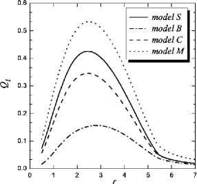
Figure 1: The quantity $Q_{t}$ as a function of radius. Its maximum value corresponds to $Q_{b}$, which gives an estimate of the relative strength of the non-axisymmetric forces. We see that the increase of the mass of the bar component (model $M$: dotted line) corresponds to “stronger bar” compared to the initial standard model (model $S$: solid line). On the other hand, when we increase the short $z$–semiaxis ($c$–parameter - model $C$: dashed line), or the intermediate $y$–semiaxis ($b$–parameter model $B$: dash-dotted line) the bar becomes weaker.

5 The two DOF model potential

The two DOF Ferrers model is described by the Hamiltonian Eq.  (11) setting $(z,p_{z})=(0,0)$, i.e.:

$$H=\frac{1}{2}(p_{x}^{2}+p_{y}^{2})+V(x,y)-\Omega_{b}(xp_{y}-yp_{x}).$$ (22)

In the two bottom inset figures of Fig. 2a, we present two typical orbits in the $(x,y)$–plane of the standard model. One is regular (bottom left inset), with initial condition: $(x,y,p_{x},p_{y})=(0,-0.625,-0.201,-0.06)\quad(\text{orbit R})$ and the other chaotic (bottom right inset), with initial condition: $(x,y,p_{x},p_{y})=(0,-0.625,-0.002,-0.24)\quad(\text{orbit C}),$ both for the Hamiltonian value $H=-0.360$. Their qualitatively different behavior is also shown in the PSS in Fig. 2a ($(y,p_{y})$–plane). The chaotic orbit C (gray points) tends to fill with scattered points the chaotic region, while the ordered orbit R (black points) creates a set of points that form a closed invariant curve, on the left part of the picture.

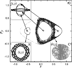
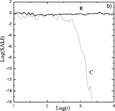
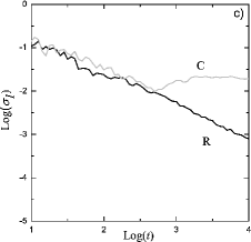
Figure 2: Analysis of orbits in the two DOF case: a) Poincaré surface of section in the $(y,p_{y})$–plane for a regular (R–black color) and a chaotic (C–gray color) orbit ($H=-0.36$). The points of the successive intersections of the regular orbit R with this plane create a closed curve, while the points of the chaotic orbit C fill with scattered points all its available region of motion. The orbits can be seen in the two inset figures in the bottom of the panel. In the top inset figure, we show examples of the three different morphologies of the regular orbits around the three main periodic orbits in the centers of the three main islands of stability. Note that the basic barred shape in the $(x,y)$–plane is mainly provided by trajectories from the central stable region, around the family of periodic orbits x1 (orbits elongated along the bar’s major axis). The other two stability islands give either elliptical-like orbits elongated perpendicular to the bar orbits (right island - family x2), or orbits which are elliptical-like but retrograde with respect the bar’s pattern speed (left island - family x4). b) The corresponding evolution of the SALI for the R and C orbits of panel a. For the chaotic one C (gray line), the SALI decays exponentially fast to zero, while for the ordered one R (black line) it fluctuates around a non-zero number. c) The corresponding evolution of the maximal Lyapunov exponents $\sigma_{1}$ for the orbits R and C. For the chaotic orbit C (gray line) this tends after some transient time to a non-zero value, while for the regular orbit R (black color) it tends linearly to zero. Note that the Log(SALI) in $y$–axis of panel b ranges from -16 to 2, while the $\text{Log}(\sigma_{1})$ in panel c ranges from -5 to 0.

In the top inset figure of Fig. 2a, we show the different morphologies of three regular orbits around the periodic orbits in the centers of the three largest islands of regular motion present in the associated PSS. The model’s basic barred shape, in the $(x,y)$–plane is mainly provided by trajectories around the main family of periodic orbits, the so–called x1 family (following the nomenclature of Contopoulos & Papayannopoulos 1980) which are orbits elongated along the bar, i.e along the $x$–axis in our case, and inside corotation. The stability island on the right gives rise to elliptical–like orbits, around the x2 family, elongated perpendicular to the bar, while the island on the left contains orbits which are elliptical-like but retrograde, very slightly elongated perpendicular to the bar and around the family x4.

We then apply the SALI method to the orbits R and C and present their different typical evolution behaviors: For the chaotic orbit C (gray curve in Fig. 2b), the SALI tends to zero $(\simeq 10^{-16})$ exponentially after some transient time, while for the regular orbit R, it fluctuates around a positive number (black curve in Fig. 2b). The corresponding mLCE and $\sigma_{1}$, for these orbits is shown in Fig. 2c, where the $\sigma_{1}$ for the regular orbit tends to zero, while for the chaotic orbit it tends to a positive number after a long integration time.

This comparison shows clearly an advantage of SALI (GALI₂), namely its ability to detect the chaotic character of an orbit faster than by simply following the mLCE, which typically takes a long time to converge. Even in our two DOF model, SALI starts to decrease exponentially after a relatively short time (in Fig. 2b, $t\leq 10^{3}$) while the corresponding mLCE $\sigma_{1}$ starts to converge to some positive non-zero value for $t\geq 10^{3}$ (see gray curve in Fig. 2c).

Exploiting the efficiency of SALI, we take initial conditions on the $(y,p_{y})$–plane (with $x=0$) and calculate the values of the index to detect very small regions of stability (or instability) more globally. We are thus able to construct a map of chaotic and regular regions, very similar to what is depicted in a PSS, but with more accuracy and higher resolution (albeit at a somewhat longer CPU time). Furthermore, as a byproduct of our application, we obtain an accurate estimate of the percentage of regular to chaotic orbits on a surface of section of the given energy.

For example, choosing different values of the energy and using a sample of 50,000 initial conditions equally spaced on the same $(y,p_{y})$–plane, we plot on the left column of Fig. 3 the PSS for $H=-0.360,-0.335,-0.300,-0.260$ and on the right the corresponding final SALI values obtained from the selected grid of initial conditions, where each point is colored according to its SALI values at the end of the integration. In the SALI plots, the light gray color corresponds to regular orbits, the black color represents the chaotic orbits/regions, while the intermediate gray shades between the two represent orbits with small rate of local exponential divergence, and/or orbits whose chaotic nature is revealed after long times, like for example the so-called sticky orbits, i.e. orbits that ”stick” onto quasiperiodic tori for long times. Note that the fraction of these orbits (which lie mainly around the borders of the islands of stability) is very small (few $\%$ of the total amount of initial conditions) and can be discerned by eye in Fig. 3 only if one focuses on these particular regions.

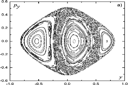
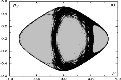
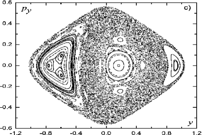
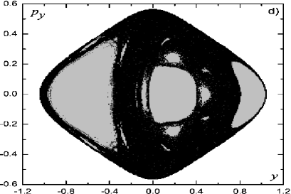
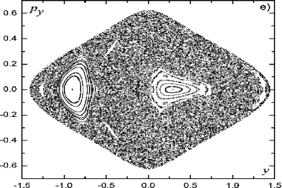
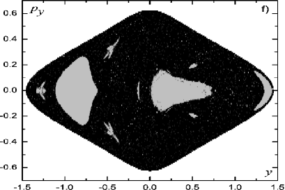
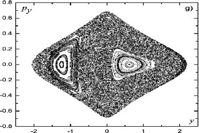
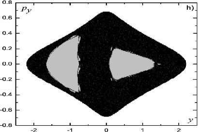
Figure 3: The PSS (left column) and SALI (right column) methods are in good agreement when surveying the same projection of the phase space. In the left column we show the PSS for the two DOF model potential with $H=-0.360$ (panel a), $H=-0.335$ (panel c), $H=-0.300$ (panel e) and $H=-0.260$ (panel g). In the right column we present regions of different values of the SALI for 50,000 initial conditions on the $(y,p_{y})$–plane for the same values of the Hamiltonian (panels b,d,f and h, respectively). The light gray colored areas correspond to regular orbits, while the dark black ones to chaotic. Note the excellent agreement between the two methods as far as the gross features are concerned, as well as the fact that the SALI can easily pick out small regions of stability which the PSS has difficulties detecting, like those around the central islands in panels b,d,f and h.

Thus, calculating from all these initial conditions the percentage of regular orbits, we are able to follow how this fraction varies as a function of the total energy. This problem was already addressed for four models by Athanassoula et al. (1983) but with fewer orbits, i.e. larger error bars. In the present model, the chosen energy values start from a regime of total order, at $H=-0.46$, up to values near the escape energy, $H_{esc}=-0.20$. The distinction between chaotic and regular orbit is that SALI$<10^{-8}$ for chaotic orbits and $\geq 10^{-8}$ for regular ones. In the latter range one does, of course, include “sticky” chaotic orbits as well. As is clear from Fig. 4, although the percentages of the regular orbits decreases sharply as the energy grows above $H=-0.4$, this tendency is reversed at higher energy values. Clearly, for $H>-0.3$, despite the fact that many stability islands have vanished, the size of the ordered domain increases because the main big island on the left of the PSS (see Fig. 3f,h) which corresponds to retrograde orbits, has become larger.

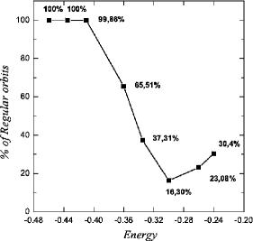
Figure 4: Percentages of regular orbits for several values of the energy ($H=$ -0.460,-0.435,-0.410,-0.360,-0.335,-0.300,-0.260,-0.240) in the two DOF Ferrers model. Note that while the fraction of the regular orbits decreases sharply as the energy grows above $H=$ -0.4, this tendency is reversed at higher energy values.

6 The three DOF model potential

We now turn to the three DOF model and begin a study of ordered and chaotic domains. Before discussing the more general results about the study of the phase space of the model, we first present in detail the behavior of our chaos indicators for some typical orbits. Let us choose a regular and a chaotic orbit and compare the efficiency of the GALI method with that of the mLCE’s.

In Fig. 5a,b we show the behavior of a chaotic orbit (C1), with initial condition: $(x,y,z,p_{x},p_{y},p_{z})=(0.5875,0.0,0.33333,0.0,0.2,0.0)$ and of a regular orbit (R1), with initial condition: $(x,y,z,p_{x},p_{y},p_{z})=(0.97917,0,0.04167,0,-0.17778,0)$. For the chaotic one, the GALI₂ (or SALI) has become almost zero for $t\simeq 10^{4}$. However, as it is clear in Fig. 5a, the higher order GALI${}_{k},\ k=5,6$, indicate the chaoticity of the orbit already by $t\simeq 10^{3}$, since they have reached very small values at that time. Note the good agreement between the predicted slopes related to its two largest Lyapunov exponents ($\sigma_{1}\approx 0.00910$ and $\sigma_{2}\approx 0.00345$) given by Eq. (8). In Fig. 5b we show the GALI indices for the regular orbit R1, where both GALI${}_{2,3}\propto$ constant and the GALI_4,5,6 decay following the power laws:

$$\text{GALI}_{4}(t)\propto\frac{1}{t^{2}},\ \text{GALI}_{5}(t) \propto\frac{1}{t^{4}},\ \text{GALI}_{6}(t)\propto\frac{1}{t^{6}},$$ (23)

obtained from Eq. (9) for $m=3$, indicating regular motion which lies on a 3D torus.

One example of a low dimensional motion (lower than 3) is provided by the regular orbit (R2), with initial condition: $(x,y,z,p_{x},p_{y},p_{z})=(0.5875,0.0,0.29770,0.0,0.33750,0.0)$. In Fig. 5c, we show the behavior of the Log(GALI) indices and their slopes for the regular orbit R2. Note that only GALI₂ remains constant while the GALI_3,4,5,6 tend to zero following power laws predicted by Eq. (9):

$$\text{GALI}_{2}(t) \propto const.,\quad\text{GALI}_{3}(t)\propto\frac{1}{t},\quad\text{GALI}_{4}(t)\propto\frac{1}{t^{2}},$$

$$\text{GALI}_{5}(t) \propto\frac{1}{t^{4}},\qquad\ \text{GALI}_{6}(t)\propto\frac{1}{t^{6}},$$ (24)

for $m=2$. This implies that the orbit’s motion lies on a 2D torus even though in three DOF Hamiltonian systems one generally expects the dimension of the torus to be three.

In Fig. 6 we show the corresponding $(x,y)$ and $(x,z)$ projections for the above C1 (1st column), R1 and R2 orbits (2nd and 3rd column respectively). The chaotic one fills up its available regime. Regarding the two regular ones, there is a clear difference reflected in their projections. The “complexity” of R1 (quasiperiodic motion on a 3D torus) is more pronounced than the one of the orbit R2 (quasiperiodic motion on a 2D torus). Thus, in such cases GALI₃ offers an extra advantage in helping us detect different “degrees” of regularity and does not serve only to distinguish between chaotic and regular motion.

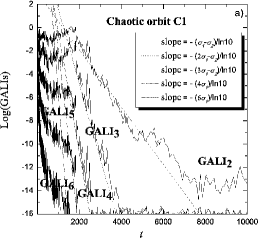
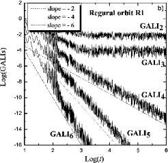
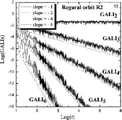
Figure 5: Distinguishing chaotic from regular motion with GALI method. a) Exponential decay of all GALIs for the chaotic orbit C1 (lin-log scale) with the predicted slopes related to its two largest Lyapunov exponents ($\sigma_{1}\approx 0.00910$ and $\sigma_{2}\approx 0.00345$). b) Slopes of GALIs for the regular orbit R1 showing that its motion lies on a 3D torus, where GALI${}_{2,3}\propto$ constant while the GALI_4,5,6 decay following a power law. c) Slopes of GALIs for the regular orbit R2 lying on a 2D torus with only GALI${}_{2}\propto$ constant.

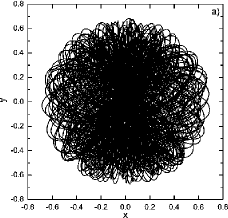
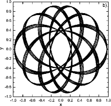
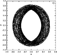
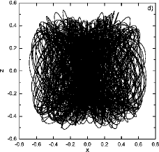
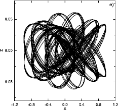
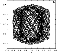
Figure 6: Two projections ($(x,y)$ and $(x,z)$–planes) of the chaotic orbit C1 (1st column) and the quasiperiodic orbits R1 (2nd column) and R2 (3rd column). Note the different “complexity” between R1, whose regular motion lies on a 3D torus, and R2, which lies on a 2D as GALI indices detected.

7 The distribution of orbits in phase space

In this section we focus on the detection and quantification of the different kinds of orbital motion (regular and chaotic) in phase (and configuration) space, as some parameters of the bar component vary. A similar study, in different potentials, was done in El-Zant & Shlosman (2002, 2003), using the Lyapunov spectra as a tool. Here we concentrate mainly in the bar component and in understanding how its different properties can affect the general stability of the system. We use a relatively large number of trajectories (50,000), more than one set of initial conditions for the survey of the phase space, and the SALI method as a chaos detector for the reasons discussed in the previous sections. We discuss the relative fraction of regular and chaotic motion not only as a function of its spatial location but also as a function of the total energy and to correlate it with the bar strength, i.e. the relative non-axisymmetric forcing.

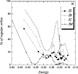
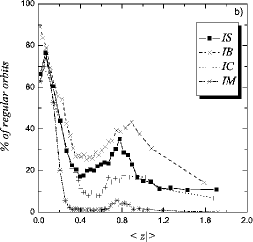
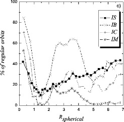
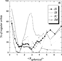
Figure 7: Percentages of regular orbits as a function of (a) the energy, (b) the averaged $<|z|>$ value, (c) the initial spherical radius $R_{spherical}$, and (d) the averaged $<R_{spherical}>$ radius of the orbit’s evolution, for models $IS$, $IB$, $IC$ and $IM$.

7.1 Initial conditions

We now need to define the sample of orbits whose properties (chaos or regularity) we will examine. The best of course would have been to draw these from a distribution function of the model. This, however, is not available, so we choose initial conditions on different grids in phase space or from the density distribution and the available energy range in the model and we measure the corresponding fraction of different kinds of motion. These percentages can depend on the choice of the sets of initial conditions and a priori are not expected to be equal. For this reason, before varying any other parameter we should consider as carefully as possible what initial conditions to choose and how well this choice “spans” the allowed phase system of the system.

We first considered sets of orbits in such a way as to favor the dynamics near the main family of periodic orbits x1 (building blocks of the bar). To this end, we launched initial conditions along the bar’s major $x$–axis with positive momenta $p_{y}$ and position ($z$) or momentum values ($p_{z}$) in the $z$–direction (distributions $I$ and $II$ below). We also considered initial conditions which follow the model’s total density $\rho$ in positions $(x,y,z)$ while their positions are arbitrary (distribution $III$ below).

Table 1: Varying parameters for all sets of initial conditions.

distribution/model	$M_{B}$	$b$	$c$
$IS,IIS,IIIS$	0.1	1.5	0.6
$IC,IIC,IIIC$	0.1	1.5	1.2
$IB,IIB,IIIB$	0.1	3.0	0.6
$IM,IIM,IIIM$	0.2	1.5	0.6

More specifically, the three different classes (distributions) of initial conditions we use here are:

• distribution $I$: 50,000 orbits equally spaced in the space $(x,z,p_{y})$ with $x\in[0.0,7.0]$, $z\in[0.0,1.5]$, $p_{y}\in[0.0,0.45]$ and $(y,p_{x},p_{z})=(0,0,0)$.

• distribution $II$: 50,000 orbits equally spaced in the space $(x,p_{y},p_{z})$ with $x\in[0.0,7.0]$, $p_{y}\in[0.0,0.35]$, $p_{z}\in[0.0,0.35]$ and $(y,z,p_{x})=(0,0,0)$.

• distribution $III$: 50,000 orbits whose spatial coordinates are chosen randomly from the density distribution of our model, using the rejection method (Press et al., 1986) within the rectangular box $-a\leq x\leq a$, $-b\leq y\leq b$, $-c\leq z\leq c$. We then draw a random value of the Hamiltonian $H$ (total energy) in the range [0, $H_{max}$], where $H_{max}$ is 1.1 times the escape energy $H_{esc}=-0.20$ defined by the zero velocity curve going through the $L_{1}$ or $L_{2}$ Lagrangian point. Then we set $(p_{y},p_{z})=(0,0)$ and we calculate the $p_{x}$–momenta by the relation: $p_{x}=H(x,y,z,p_{y},p_{z})$ (keeping the positive solution). Note that in this case instead of giving $p_{y}$–momenta we tried $p_{x}$. This choice allows us to check how a different way of populating the phase space may affect the relative fraction of regular and chaotic motion. This third distributions has a better representation of the density, but still is arbitrary with respect to the velocities.

Details of our distributions/models can be found in Table 1. In the next sections we start by studying the distribution of regular and chaotic motion in phase space, for different choices of initial conditions, different bar parameters (sizes, mass and pattern speed). We also briefly study the distribution as a function of energy and of location in configuration space.

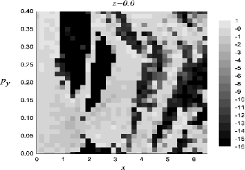
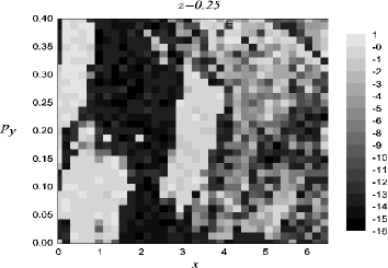
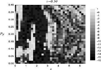
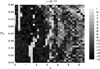
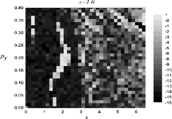
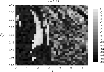
Figure 8: Slices of the $(x,p_{y})$–plane for different $z$ values. Dark regions correspond to chaotic initial conditions, light gray to regular ones and intermediate colors to orbits with a small rate of local exponential divergence, and/or orbits whose chaotic nature is revealed after long times, like for example the so-called sticky orbits. The gray-scale bar represents the values of the SALI in logarithmic scale.

7.2 Percentages of regular orbits vs. energy

We next examine the variation of the percentages of regular and chaotic orbits as a function of the energy and we show the results in Fig. 7a. We first divided the energy interval into 30 subintervals, each containing an equal number of orbits. In every subinterval we calculated the percentages of regular and chaotic orbits. In Fig. 7a we plot the percentage of regular orbits for energies up to $H\simeq-0.15$, i.e. up to a value somewhat beyond the escape energy for all models under study. Generally, we observe that the fraction of regular orbits decreases as the energy increases. An important peak, however, occurs before the escape energy, so that for ($H>-0.20$) the fraction of regular orbits increases again! This non–monotonic behavior is related to the growth of the islands around some basic stable periodic orbits in the phase space and is similar to what was observed in the two DOF model, comparing the fraction of regular orbits for the common energy interval, i.e. up to $H\leq-0.24$ (see Fig. 4).

Picking another set of initial conditions we find similar qualitative results with some small quantitative differences. Hence, we find the same behavior when studying the models of distribution $II$, i.e. regular motion is dominant for small generally energies, then a decrease and then a peak. Distribution $III$ manifests the same trend for small energies while the peak is less intense compared to the other two distributions.

7.3 Spread of regular orbits in configuration space

We also explored the way in which regular and chaotic orbits are distributed along the $z$–direction of the configuration space. Following the evolution of each orbit, we calculated the mean absolute value of their $z$–coordinate ($<|z|>$) and plot in Fig. 7b the fraction of regular orbits as a function of the $<|z|>$ for the models of distribution $I$. It clearly follows from these results that the intervals relatively near the $(x,y)$–plane ($<|z|>~{}<0.35$) contain mainly regular orbits, while those with larger values of mean absolute distance $z$ are mostly chaotic. Similar qualitative results are obtained for distribution $II$ (not shown here). Checking distribution $III$ we find good match for the relative fraction of regular motion for relatively small $<|z|>$ (up to 0.4) with the other models. For intermediate values ($0.4<~{}<|z|>~{}<1.5$) the motion is mostly chaotic while we don’t have orbits reaching larger values, which is due to the way the initial conditions are given.

We also looked at these percentages as a function of the initial spherical radius ($R_{spherical}=\sqrt{x_{0}^{2}+y_{0}^{2}+z_{0}^{2}}$) and the mean spherical radius over the evolution of the orbits ($<R_{spherical}>$). Again, dividing the total range of the $R_{spherical}$ values in 30 subintervals, we calculated the percentages of regular orbits as a function of the mean $R_{spherical}$ value in each subinterval. We find that the fraction of regular orbits for all models decreases sharply with increasing $R_{spherical}$ up to $R_{spherical}<1.5$, where it reaches a minimum (see Fig. 7c). For $1.5<R_{spherical}<7$ it starts to increase gradually almost monotonically for model $IS$ and with some rather week fluctuations for $IC$. Note that the model $IB$ possesses a relatively large fraction of regular motion within the interval $2.5<R_{spherical}<4.5$ as well. Model $IM$ follows a similar trend, but with a different scale than $IB$, containing its larger fraction of regular motion in the same roughly intervals, while for larger $R_{spherical}$ the motion is mainly chaotic. This result is in good agreement with the results in Fig. 7d, where the horizontal axis corresponds to the value of the mean spherical radius over the evolution time of the orbits. As previously, distribution $II$ confirms well this behavior while distribution $III$ is in good agreement for relatively small radial distances from the center of the galaxy and diversifies for larger ones.

7.4 Fraction of regular motion as a function of distance from the equatorial plane

We then examine whether the orbital motion is more “regular” near the $(x,y)$–plane or far from it and how this relates to their behavior as a function of $<|z|>$ discussed in the subsection 7.3 and Fig. 7b. For this, we took the set of initial conditions from distribution $I$ (version $IC$ in this example) with initial conditions given in the space $(x,z,p_{y})$ and create a mesh in the $(x,p_{y})$–plane with different slices in the $z$–direction that start from $z=0$ up to $z=1.25$ with $step=0.25$. In Fig. 8, we see that as the distance of the initial conditions from the equatorial plane increases (from top to bottom row and from left to right panels), large islands of stability in the $(x,p_{y})$–plane start to shrink, when $x$ is between 0 and 2. This trend is almost monotonic up to the $z$–slice $z\approx 1$ (Fig. 8, third row, left panel). For $z=1.25$ (Fig. 8, third row, right panel) the stability region, lying between $x=1.5$ and $x=2$ starts to grow. This result turns out to be in good agreement with the one in Fig. 7b, where we plot the percentages of regular orbits as a function of $<|z|>$. This trend, as expected, is similar for the other two different sets of initial conditions (distributions $IIC$ and $IIIC$), since the model parameters remain the same.

7.5 Percentages of regular orbits vs pattern speed

Furthermore, choosing one class of initial conditions (distribution $IS$), we compare different models for several values of the bar’s pattern speed $\Omega_{b}$, keeping the remaining parameters constant. In this study, we try to explore the effect of the value of the pattern speed on the percentages of globally ordered or chaotic behavior of the system.

Based on the structure and crowding of the periodic orbits, Contopoulos (1980) showed that bars have to end before corotation, i.e. that $r_{L}>a$, where $r_{L}$ the Lagrangian, or corotation, radius. A similar result was reached from the calculation of the self-consistent response to a bar forcing (Athanassoula, 1980). These two results are very useful, since they set a lower limit to the corotation radius, which can thus not be smaller than the bar length, but give no information on an upper limit. Comparing the shape of the observed dust lanes along the leading edges of bars to that of the shock loci in hydrodynamic simulations of gas flow in barred galaxy potentials, Athanassoula (1992a, b) was able to set both a lower and an upper limit to the corotation radius, namely $r_{L}=(1.2\pm 0.2)a$. This restricts the range of possible values of the pattern speed for our model, from $\Omega_{b}=0.0367$, that corresponds to the Lagrangian radius $r_{L}=1.4a$, to $\Omega_{b}=0.0554$, that corresponds to $r_{L}=1.0a$. Using these extreme values, and the three intermediate frequencies: $\Omega_{b}=0.0403$, $\Omega_{b}=0.0444$ and $\Omega_{b}=0.0494$, that correspond to the Lagrangian radii $r_{L}=1.3a$, $r_{L}=1.2a$ and $r_{L}=1.1a$, respectively, we investigated how the value of the pattern speed affects the system and found that as $\Omega_{b}$ increases the percentage of the regular orbits decreases relatively weakly. The corresponding results are given in Table 2. It turns out that the variation of the pattern speed does not affect drastically the relative fraction of regular and chaotic motion. One would probably need to try more extreme values of $\Omega_{b}$, beyond the upper and lower limits of the corotation radius, in order to see a significant change. Such values, however, would be unrealistic for real galaxies.

Table 2: Models with different pattern speeds $\Omega_{b}$.

model	$\Omega_{b}$	$r_{L}$	% of Regular orbits
$I\Omega_{1}$	0.0367032	1.4a	28.39
$I\Omega_{2}$	0.0403014	1.3a	27.63
$I\Omega_{2}$	0.0444365	1.2a	27.26
$I\Omega_{4}$	0.0493654	1.1a	26.55
$I\Omega_{5}$	0.0554349	1.0a	25.55

7.6 Fraction of regular and chaotic trajectories

In this section and in Fig. 9, we investigate the amount of regular motion in the phase space for all the three sets of initial conditions (distributions $I$, $II$ and $III$), varying the axial ratios ($b/a$ or $c/a$ parameters) and the mass ($M_{B}$ parameter) of the bar component, as described in Table 1. In all distributions we used 50,000 initial conditions and we employed the bootstrap–method (Press et al., 1986) on several subsamples to make sure that this number is sufficiently high to provide reliable information. Computing the distributions of regular and chaotic orbits for the above classes of initial conditions we find the following:

7.6.1 Percentages for distribution $I$

Before starting with the full 3D model, we first measured the percentages of regular orbits in the 2D model. We use initial conditions equally spaced in $(x,p_{y})$, with $(y,p_{x})=(0,0)$, $x\in[0.0,7.0]$ and $p_{y}\in[0.0,0.45]$. We find relative fractions of regular motion equal to $45.40\%$ for model $IM$, $53.43\%$, for model $IS$, $92.43\%$ for model $IB$ and $64.43\%$ for model $IC$. This shows that at least in the 2D case, the massive bar model ($IM$) has the highest fraction of chaotic orbits, followed by the standard distribution $IS$. The two models with the extended short ($IC$), or intermediate axis ($IB$) have the least chaos.

Let us now turn to the full 3D orbital coverage. In Fig. 9a we present the percentages of the regular orbits for the various sets of initial conditions of the distribution $I$. Comparing the percentages, we see that increasing the mass of the bar in model $IM$ increases chaotic behavior. This confirms the results obtained above and in Athanassoula et al. (1983) for the two DOF case. On the other hand, when the bar is thicker (model $IC$), i.e. the length of the $z$–axis larger, the system becomes more regular. Finally, the corresponding results for a fatter bar, i.e. with larger $y$–axis (model $IB$) demonstrate that the increase of the intermediate axis of the bar also provides the system with more ordered behavior.

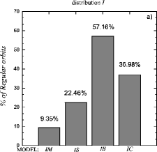
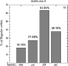
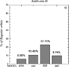
Figure 9: Percentages of regular orbits (SALI$\geq 10^{-8}$) for distribution $I$ (left panel), $II$ (middle panel) and $III$ (right panel) of initial conditions for all the different model versions, where the bar mass and the length of its intermediate and minor (vertical) semi-axes are varied. Generally, when the bar mass increases the model tends to be more chaotic, while when the size of the bar semi-axes ($b$ or $c$ parameters) increases the fraction of regular motion grows. The small difference in the trends between models $IS\rightarrow IC$ and $IIIS\rightarrow IIIC$ is due to the different way in which the sample of initial conditions in phase space is chosen.

Comparing the 2D and 3D cases presented above, we note that the trends we find are the same, but that the relative fractions of regular orbits are somewhat higher in the 2D case. We will discuss this further towards the end of the section.

7.6.2 Percentages for distribution $II$

Similarly, in Fig. 9b, we present percentages of the regular orbits for initial conditions selected for distribution $II$ and models $S$, $M$, $B$ and $C$. As before, the increase of the bar mass (model $IIM$) causes more extensive chaos, while for a thicker bar or fatter bar (models $IIB$ and $IIC$), the system is again more regular. It is thus clear that the results of distributions $I$ and $II$ are similar, presumably dues to the fact that they contain initial conditions that cover the phase space in a similar manner, i.e. they favor the region around the x1 family of periodic orbits.

7.6.3 Percentages for distribution $III$

Finally, we plot in Fig. 9c the percentages of regular orbits for several sets of initial conditions from distribution $III$. A first general observation is that the fraction of ordered motion is significantly smaller than is distributions I and II, for all models. The basic reason for this difference is related to the way that the momenta of the positions are given in this distribution of initial conditions. In particular, all the orbits in this case are launched with a $p_{x}$ momentum instead of a $p_{y}$ as in distributions $I$ and $II$. As a consequence, the big island of stability around the main family of periodic orbits x1 is populate with fewer orbits and thus in general more chaotic orbits are launched and measured. Nevertheless, again the increase of the bar mass in the $IIIM$ model results in more chaotic behavior. As for the $IB$ model, a thicker bar in the $y$–direction turns out to make the system more regular. Regarding the case of larger $z$–semiaxis (model $IIIC$), we notice a small decrease in the percentages of regular orbits (9.74$\%$ now, from 10.46$\%$). It turns out that this particular different distribution of initial conditions doesn’t reveal quite the same trend as in the previous cases ($IS\rightarrow IC$ and $IIS\rightarrow IIC$).

Concluding this section dedicated to the dynamical study of regular and chaotic motion in the phase space is that their corresponding fraction is basically related to the way that one populates the main stable (or unstable) periodic orbits of the system. We find that motion near the plane is generally stable (non chaotic) and that trajectories spending the largest fraction of time at large $z$ are usually chaotic (with large Lyapunov exponents). These results are in agreement with the results obtained by El-Zant & Shlosman (2002, 2003) for different models. The increase of the bar mass leads to more chaotic motion in the phase space as found in Athanassoula et al. (1983) for a two DOF model, while in general the increase of the bar $y$ or $z$–semiaxis leads to more regularity.

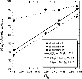
Figure 10: The relative fraction of chaotic motion as a function of bar strength $Q_{b}$ increases (see Fig.1). Filled squares ($\blacksquare$) correspond to the models $M$, $S$, $C$ and $B$ (from right to left, respectively) for distribution $I$. while filled triangles ($\blacktriangledown$) are for distribution $II$ and filled circles ($\bullet$) for distribution $III$.

7.7 The effect of bar strength

Reviewing the above percentages of regular (and chaotic) motion in phase space, we see that they change in the same way when the basic parameters and properties of the model are varied. In order to understand this better we examine next the effect of the bar strength, measuring it as discussed in Section 4, i.e. from the relative strength of the non-axisymmetric forcing. In Fig. 10 we plot the relative fraction of chaotic motion as a function of bar strength $Q_{b}$. Black filled squares correspond to distribution $I$, filled triangles to distribution $II$ and filled circles to distribution $III$. This figure reveals that, provided the choice of initial conditions for the orbits is the same or similar, there is a tight correlation between the two quantities. the amount of chaos increases with increasing bar strength, as intuitively expected. What is unexpected, however, is how tight all these correlations are, with rank correlation coefficients $\sim-0.936$ for all distributions.

Fig. 10 also shows that, except for the bar strength, the distribution of initial conditions chosen is also important. Distributions $I$ and $II$ differ little and their best fitting straight lines are roughly parallel and little displaced from each other. This is in good agreement with our previous statement (subsect. 7.1) that they both cover well the regular orbits trapped around the stable orbits of the x1 family, which are in fact the backbones of the bar (Athanassoula et al., 1983). On the other hand, distribution $III$ has a much higher fraction of chaotic orbits, as could also be seen from Fig. 9c, attesting that the corresponding distribution of initial conditions is more chaotic, for the reasons we already described.

8 Conclusions

In this paper, paper I, we studied the detection and distribution of regular and chaotic motion in the phase space of barred galaxy models. Our results referring to the dynamical properties of the 2D/3D model with a Ferrers bar can be summarized as follows:

1. We applied successfully the GALI method to distinguish both qualitatively and quantitatively between regular and chaotic orbits. We showed its efficiency and its advantage in detecting fast and accurately the chaotic nature of a trajectory.

2. In 2D systems, using the SALI (GALI₂) method, we were able to identify efficiently and fast tiny regions of regular or chaotic motion, which are not clearly visible on PSSs.

3. Using GALI_2,3 we detected regular motion in low dimensional tori, i.e. examples of regular orbits of the three DOF Ferrers’ model that lie on a 2D torus, while the torus’ expected dimension is generally three. Concerning chaotic orbits, the GALI_3,4,5,6 indices decay faster than SALI and are able to detect chaos at early times well before this is evident from the calculation of the mLCE.

4. We also tried different models and different distributions of initial conditions for the orbits to test the fraction of regular and chaotic motion in various cases. We found that regular orbits are generally dominant at relatively small radial distances from the center of the galaxy and at small distances from the equatorial plane.

5. We tested the effect of varying the bar pattern speed for our standard model and found that, within a realistic range of values, this parameter does not affect much the phase space dynamics. Within these limits, we found that the fraction of regular motion varies only by about 3 per cent, in the sense that the bars at the slow limit of the realistic range have more regular motion than the bars in the fast limit.

6. We varied the values of the main parameters of our models, such or the mass and the axial ratio of the bar component (in the 3D model). Chaos turns out to be dominant in galaxy models whose bar component is more massive, while models with a thicker or fatter bar present generally more regular behavior although the initial conditions are given can in general affect somewhat the relative percentages.

7. We found a very strong correlation (rank correlation coefficient at $\sim$0.94) between the fraction of chaotic orbits and the relative strength of the non-axisymmetric forcing. This holds for all our three initial conditions distributions taken individually, even though they were specifically chosen so as to represent different types of orbits. We can thus conclude that strong non-axisymmetric forcings (i.e. strong bars) are the main cause of the presence of large amount of chaotic motion in phase space.

In our next paper of this series (paper II) we focus on the significance of the “different degrees” of chaotic motion, like the strong and weak chaos, and their significance from an astronomical point of view. The fact that many “sticky”/chaotic orbits often persist and behave in a regular manner for very large time intervals, before showing their chaoticity, makes them astronomically important for supporting the galaxy structure. We present there a first approach in filtering these weak chaotic orbits from the strongly chaotic ones and classify them observationally as effectively ordered motion.

9 Acknowledgements

We would like to thank Ch. Skokos, T. Bountis, A. Bosma, M. Romero-Gómez and P.A. Patsis for their fruitful comments and discussions on this work. We also thank the referee, P.M. Cincotta, for his report, which helped us improve the clarity of the paper. T. Manos acknowledges the “Karatheodory” graduate student fellowship No B395 of the University of Patras and funds from the Marie Curie fellowship No HPMT-CT-2001-00338 to Marseille observatory. Visits between the Marseille and Patras team members were partially funded by the region PACA in France. This work was partially supported by the grant ANR-06-BLAN-0172.

References

- Antonopoulos & Bountis (2006) Antonopoulos, Ch., Bountis, T., 2006, Phys. Rev. E, 73, 056206
- Antonopoulos & Bountis (2006) Antonopoulos, Ch., Bountis, T., 2006, ROMAI Journal, 2(2), 1
- Antonopoulos et al. (2006) Antonopoulos, Ch., Bountis, T., Skokos, Ch., 2006, Int. J. Bif. Chaos, 16(6), 1777
- Athanassoula (1980) Athanassoula, E. 1980, A&A, 88, 184
- Athanassoula et al. (1983) Athanassoula, E., Bienayme, O., Martinet, L., Pfenniger, D., 1983, A&A, 127, 349
- Athanassoula (1992a) Athanassoula, E., 1992a, MNRAS, 259, 328
- Athanassoula (1992b) Athanassoula, E., 1992b, MNRAS, 259, 354
- Athanassoula et al. (2009a) Athanassoula, E., Romero-Gómez, M., Masdemont, J. J, 2009a, MNRAS, 394, 67
- Athanassoula et al. (2009b) Athanassoula, E., Romero-Gómez, M., Bosma, A., Masdemont, J. J., 2009b, MNRAS, 400, 1706
- Athanassoula et al. (2010) Athanassoula, E., Romero-Gómez, M., Bosma, A., Masdemont, J. J., 2010, MNRAS, 407, 1433
- Benettin et al. (1980a) Benettin, G., Galgani, L., Giorgilli, A., Strelcyn, J.-M., 1980, Meccanica, 9
- Benettin et al. (1980b) Benettin, G., Galgani, L., Giorgilli, A., Strelcyn, J.-M., 1980, Meccanica, 21
- Bountis & Skokos (2006) Bountis, T., Skokos, Ch., 2006, Nucl. Instr. Meth. - Sect. A, 561, 173
- Bountis et al. (2009) Bountis, T., Manos, T., Christodoulidi, H., 2009, J. Comp. Appl. Math., 227, 17
- Buta et al. (2003) Buta, R., Block, D. L., Knapen, J. H., 2003, AJ, 126, 1148
- Buta et al. (2004) Buta, R., Laurikainen, E., Salo, H., 2004, AJ, 127, 279
- Buta et al. (2005) Buta, R., Vasylyev, S., Salo, H., Laurikainen, E., 2005, AJ, 130, 506
- Capuzzo-Dolcetta et al. (2006) Capuzzo-Dolcetta, R., Leccese, L., Merritt, D., Vicari, A., 2007, ApJ, 666, 165
- Christodoulidi & Bountis (2006) Christodoulidi, H., Bountis, T., 2006, ROMAI Journal, 2(2), 37
- Cachucho et al. (2010) Cachucho, F., Cincotta, P. M., Ferraz-Mello, S., 2010, CMDA, 108, 35
- Cincota & Simó (2000) Cincota, P. M., Simó, C., 2000, Astron. Astroph. Suppl. Ser., 147, 205
- Cincota et al. (2003) Cincota, P. M., Giordano, C. M., Simó, C., 2003, Physica D, 182, 151
- Cincota & Giordano (2008) Cincotta, P. M., Giordano, C. M., 2008, In the book Nonlinear Phenomena Research, Nova Science Publishers, 319
- Contopoulos & Papayannopoulos (1980) Contopoulos, G., Papayannopoulos, Th., 1980, A&A, 92, 33
- Contopoulos (1980) Contopoulos G., 1980, A&A, 81, 198
- Contopoulos et al. (1995) Contopoulos, G., Grousousakou, E., Voglis, N., 1995, A&A, 304, 374
- Contopoulos & Voglis (1996) Contopoulos, G., Voglis, N., 1996, Celest. Mech. Dyn. Astron., 64, 1
- Contopoulos & Voglis (1997) Contopoulos, G., Voglis, N., 1997, A&A, 317, 73
- Contopoulos (2002) Contopoulos, G., 2002, Order and chaos in dynamical astronomy, Springer-Verlag, Berlin
- Contopoulos & Harsoula (2008) Contopoulos, G., Harsoula, M., 2008, Int. J. Bif. Chaos, 18, 2929
- Durbala et al. (2009) Durbala, A., Buta, R., Sulentic, J. W., Verdes-Montenegro, L., 2009, MNRAS, 397, 1756
- El-Zant & Shlosman (2002) El-Zant, A., Shlosman, I., 2002, ApJ, 577, 626
- El-Zant & Shlosman (2003) El-Zant, A., Shlosman, I., 2003, ApJ, 595, L41
- Ferrers (1877) Ferrers, N. M., 1877, Quart. J. Pure Appl. Math., 14:1
- Froeschlé et al. (1997) Froeschlé, C., Lega, E., Gonzi, R., 1997, Celest. Mech. Dyn. Astron., 67, 41
- Froeschlé & Lega (1998) Froeschlé, C., Lega, E., 1998, A&A, 334, 355
- Giordano & Cincotta (2004) Giordano, C. M., Cincotta, P. M., 2004, A&A, 423, 745
- Harsoula & Kalapotharakos (2009) Harsoula, M., Kalapotharakos, C., 2009, MNRAS, 394, 1605
- Kalapotharakos et al. (2004) Kalapotharakos, C., Voglis, N., Contopoulos, G., 2004, MNRAS, 428, 905
- Kalapotharakos et al. (2008) Kalapotharakos, C., Efthymiopoylos, C., Voglis, N., 2008, MNRAS, 383, 971
- Kaufmann & Contopoulos (1996) Kaufmann, D. E., Contopoulos, G., 1996, A&A, 309, 381
- Laskar (1990) Laskar, J., 1990, Icarus, 88, 266
- Laskar et al. (1992) Laskar, J., Froeschlé, C., Celletti, A., 1992, Physica D, 56, 253
- Laskar (1993) Laskar, J., 1993, Physica D, 67, 257
- Laurikainen et al. (2004) Laurikainen, E., Salo, H., Buta, R., 2004, ApJ, 607, 103
- Lieberman & Lichtenberg (1992) Lieberman, M., Lichtenberg, A., 1992, Regular and Stochastic Motion, Springer Verlag, Berlin
- Macek et al. (2010) Macek, M., Dobeš, J., Cejnar, P., 2010, Phys. Rev. C, 82, 014308
- Manos et al. (2008a) Manos, T., Skokos, Ch., Athanassoula, E., Bountis, T., 2008a, Nonlinear Phenomena in Complex Systems, 11(2), 171
- Manos et al. (2008b) Manos, T., Skokos, Ch., Bountis, T., 2008b, Proceedings of the conference Chaos, Complexity and Transport: Theory and Applications, edited by Chandre C., Leoncini X. and Zaslavsky G., World Scientific Publishing, 356
- Manos & Athanassoula (2008) Manos, T., Athanassoula, E., 2008, Proceedings of the international conference Chaos in Galaxies, edited by Contopoulos G. and Patsis P., Springer-Verlag, Berlin-Heidelberg (ASSP), 115
- Manos et al. (2008c) Manos, T., Skokos, Ch., Bountis, T., 2008c, Proceedings of the international conference Chaos in Galaxies, edited by Contopoulos G. and Patsis P., Springer-Verlag, Berlin-Heidelberg (ASSP), 376
- Manos & Ruffo (2010) Manos, T., Ruffo, S., 2010, Trans. Th. and Stat. Phys., (accepted - eprint arXiv:1006.5341)
- Miyamoto & Nagai (1975) Miyamoto, M., Nagai, R., 1975, PASJ, 27, 533
- Oseledec (1968) Oseledec, V. I., 1968, Trans. Moscow Math. Soc., 19, 197
- Panagopoulos et al. (2004) Panagopoulos, P., Bountis, T., Skokos, Ch., 2004, J. Vib. & Acoust., 126, 520
- Patsis (2006) Patsis, P. A., 2006, MNRAS, 369, L56
- Patsis et al. (1997) Patsis, P. A., Athanassoula, E., Quillen, A. C., 1997, ApJ, 483, 731
- Patsis et al. (2002) Patsis, P. A., Skokos, Ch., Athanassoula, E., 2002, MNRAS, 337, 578
- Patsis et al. (2003a) Patsis, P. A., Skokos, Ch., Athanassoula, E., 2003a, MNRAS, 342, 69
- Patsis et al. (2003b) Patsis, P. A., Skokos, Ch., Athanassoula, E., 2003b, MNRAS, 346, 1031
- Pettini (2007) Pettini, M., 2007, Geometry and topology in Hamiltonian dynamics and statistical mechanics, Springer Verlag, Berlin
- Pfenniger (1984) Pfenniger, D., 1984, A&A, 134, 373
- Plummer (1911) Plummer, H. C, 1911, MNRAS, 71, 460
- Press et al. (1986) Press, W. H., Teukolsky, S. A., Vetterling, W. T., Flannery, B. P., Numerical recipes in Fortran 77: The art of scientific computing, Cambridge: University Press, Second Edition, Volume 1 of Fortran Numerical Recipes
- Romero-Gómez et al. (2006) Romero-Gómez, M., Masdemont, J. J., Athanassoula, E., García-Gómez, C., 2006, A&A, 453, 39.
- Romero-Gómez et al. (2007) Romero-Gómez, M., Athanassoula, E., Masdemont, J. J., García-Gómez, C., 2007, A&A, 472, 63
- Romero-Gómez et al. (2009) Romero-Gómez, M., Masdemont, J. J., García-Gómez, C., Athanassoula, E., 2009, Communications in Nonlinear Science and Numerical Simulations, 14, 412
- Skokos (2001) Skokos, Ch. 2001, J. Phys. A: Math. Gen., 34, 10029
- Skokos et al. (2002a) Skokos, Ch., Patsis, P. A., Athanassoula, E., 2002a, MNRAS, 333, 847
- Skokos et al. (2002b) Skokos, Ch., Patsis, P. A., Athanassoula, E., 2002b, MNRAS, 333, 861
- Skokos et al. (2002) Skokos, Ch., Antonopoulos, Ch., Bountis, T., Vrahatis, M., 2002, in Proceedings of the 4th GRACM, edited by Tsahalis D.T., IV, 1496
- Skokos et al. (2003a) Skokos, Ch., Antonopoulos, Ch., Bountis, T., Vrahatis, M., 2003a, Prog. Theor. Phys. Suppl., 150, 439
- Skokos et al. (2003b) Skokos, Ch., Antonopoulos, Ch., Bountis, T., Vrahatis, M., 2003b, Proceedings of the Conference Libration Point Orbits and Applications, edited by Gomez G., Lo M.W. and Masdemont J.J., World Scientific, 653
- Skokos et al. (2004) Skokos, Ch., Antonopoulos, Ch., Bountis, T., Vrahatis, M., 2004, J. Phys. A, 37, 6269
- Skokos et al. (2007) Skokos, Ch., Bountis, T., Antonopoulos, Ch., 2007, Physica D, 231, 30
- Skokos et al. (2008) Skokos, Ch., Bountis, T., Antonopoulos, Ch., 2008, Eur. Phys. J. Sp. Top., 165, 5
- Skokos (2010) Skokos, Ch., 2010, Lect. Notes Phys., 790, 63
- Stránský et al. (2009) Stránský, P., Hrus̆ka, P., Cejnar, P., 2009, Phys. Rev. E, 79, 046202
- Széll et al. (2004) Széll, A., Érdi, B., Sándor, Zs., Steves B., 2004, MNRAS, 347, 380
- Tsoutsis et al. (2009) Tsoutsis, P., Kalapotharakos, C., Efthymiopoulos, C., Contopoulos, G., 2009, A&A, 495, 743
- Valluri et al. (2010) Valluri, M., Debattista, V.P., Quinn, T., Moore, B., 2010, MNRAS, 403, 525
- Voglis et al. (1998) Voglis, N., Contopoulos, G., Efthymiopoylos, C., 1998, Phys. Rev. E, 57, 372
- Voglis et al. (1999) Voglis, N., Contopoulos, G., Efthymiopoylos, C., 1999, Celest. Mech. Dyn. Astron., 73, 211
- Voglis et al. (2002) Voglis, N., Kalapotharakos, C., Stavropoulos, I., 2002, MNRAS, 337, 619
- Voglis et al. (2006a) Voglis, N., Stavropoulos, I., Kalapotharakos, C., 2006a, MNRAS, 372, 901
- Voglis et al. (2006b) Voglis, N., Tsoutsis, P., Efthymiopoulos, C., 2006b, MNRAS, 373, 280
- Voglis et al. (2007) Voglis, N., Harsoula M., Contopoulos, G, 2007, MNRAS, 381, 757