The Mass Mixing Length in Convective Stellar Envelopes

Abstract

The scale length over which convection mixes mass in a star can be calculated as the inverse of the vertical derivative of the unidirectional (up or down) mass flux. This is related to the mixing length in the mixing length theory of stellar convection. We give the ratio of mass mixing length to pressure scale height for a grid of 3D surface convection simulations, covering from 4300 K to 6900 K on the main-sequence, and up to giants at $\log g=2.2$, all for solar composition. These simulations also confirm what is already known from solar simulations, that convection doesn’t proceed by discrete convective elements, but rather as a continuous, slow, smooth, warm upflow and turbulent, entropy deficient, fast down drafts. This convective topology also results in mixing on a scale as that of the classic mixing length formulation, and is simply a consequence of mass conservation on flows in a stratified atmosphere.

1 Introduction

For stellar structure and evolution calculations (e.g., Iben, 1967), models for the relevant energy-transport mechanisms are needed. In the interior, radiative or conductive transfer of energy is trivial, although the atomic physics going into the opacities and conductivities are not. A satisfactory description of convection in a manner amenable to stellar structure calculations, however, has proven elusive. Stellar modelers usually use the mixing length theory (MLT) (Böhm-Vitense, 1958; Gough, 1977), which despite its simplicity and many shortcomings, has been highly successful in matching a variety of stellar observations. In this model, convection is thought of as a collection of fluid parcels that travel a distance equal to the mixing length and then thoroughly mix with the surrounding ambient medium, sharing their energy. The MLT picture is completely symmetric, so the upward flow of buoyant warm elements is accompanied by an equal number of cooler and over-dense elements moving inward. In these calculations the mixing length is a free parameter and is specified as a multiple of the pressure scale height $H_{P}=P/\rho g$, where $P$ is the pressure, $\rho$ is the density and $g$ is the gravitational acceleration. In general, there are also free parameters specifying the geometry of the fluid parcel – the ratio of its horizontal to vertical size and another specifying the lateral radiative transfer between convective elements and the ambient medium. The simple mixing length model is used due to a lack of better alternatives and because it is quick to compute. Its primary function is to determine the entropy of the deep, efficient and nearly adiabatic part of the convection zone in the star. If the magnitude of the mixing length and the other parameters could be specified a priori, simple mixing length theory would be capable of fulfilling this function. However, there is little guidance from theory as to their values.

In addition, the mixing length model suffers from several other problems: it does not allow for overshooting motions that mix material into the surrounding stable layers, it does not allow for turbulence, it does not allow for asymmetry between upflows and downflows, especially the large temperature difference near the surface and its effect on opacities and radiative transfer. These are all phenomena that, according to realistic 3D simulations, contribute to the atmospheric entropy jump and hence, the adiabat of the deep, efficient convection. Several attempts have been made to improve the mixing length model. Some have taken the mixing length to be the distance to the nearest boundary (Stothers & Chin, 1997), some have introduced a two-stream model with separate properties of the upflows and downflows (Nordlund, 1976), some have introduced the idea of a spectrum of sizes of the convective cells (Canuto & Mazzitelli, 1991).

Several attempts have been made to determine the appropriate value of the ratio of mixing length to pressure scale height by matching theoretical and observed evolutionary tracks in the Hertzsprung-Russell diagram (Chieffi et al., 1995; Stassun et al., 2004), by matching observed and model properties of binary systems (Fernandes et al., 1998, 2002; Montalbán et al., 2004), and red giant temperatures (Ferraro et al., 2006). There have also been a few attempts to determine the mixing length parameter by comparing one-dimensional mixing length stellar model calculations with two- and three-dimensional numerical simulations of stellar convection by either matching entropy in the adiabatic portion of the convection zone (Ludwig et al., 1999; Freytag & Salaris, 1999) or by matching temperature and density at a given pressure in the interior (Trampedach et al., 1999, 2011b).

Mixing length theory works reasonably well for determining the thermal structure of convection zones because real mixing of mass occurs in stratified convection. Stars are stratified. Their density decreases from their center to their surface in order to produce a pressure gradient to balance the inward pull of gravity. In order to conserve mass in such a stratified medium, most of the ascending material must turnover and head back down within about a density scale height (Stein & Nordlund, 1989). Thus, mixing really does occur on the order of a density scale height.

It is possible to easily and unambiguously calculate the mass mixing length from computational fluid dynamic simulations of stellar convection. Such simulations, when they employ realistic equations of state to relate the pressure to the density and internal energy or temperature and employ sufficiently accurate treatment of radiative transfer to determine the heating and cooling, have as free parameters only the resolution of the computational grid used and the magnitude of the diffusion used to stabilize the calculations. These parameters, however, are not free to be adjusted to match observations. The diffusion is minimized against the requirement of a numerically stable simulation, and the resolution is chosen as a trade-off between resolving features in the photosphere and computational cost. We would not lower the resolution or increase the diffusion to give a better match to some observations.

In this paper, we present results of such mass mixing calculation for a homogeneous sample of convection simulations, covering a large part of the Hertzsprung-Russell diagram for which stars have convective envelopes. The simulations form an irregular grid, covering 4 500–6 900 K on the main sequence and going up to giants with $\log g=2.2$ and $T_{\rm eff}=$4 300-5 000 K, all with solar composition. The simulations employ the Mihalas-Hummer-Däppen equation of state (Hummer & Mihalas, 1988), line-opacity from Kurucz (1992) and continuum opacities largely from the Marcs stellar atmosphere package (Gustafsson et al., 1975), but with many improvements. The simulations are described in more detail in Trampedach et al. (2011a, b).

2 Mass Mixing Length

Figure 1: Uni-directional downward mass flux as a function of the mean pressure for the stars in our sample. The break in the mass flux near pressures of $10^{5}$ dyn/cm² occurs in the photosphere. The effect of the bottom boundary can be seen as a small downturn near the high pressure end of the traces.

The mass mixing length, the distance over which, because of mass conservation, most of the ascending fluid turns over and starts to descend, is the inverse of the logarithmic derivative of the unidirectional mass flux (Stein et al., 2009),

$$\ell_{m}(r) = \left|{\rm d}\ln F_{\uparrow m}(r)/{\rm d}r\right|^{-1}$$ (1)

$$= \left|{\rm d}\ln F_{\downarrow m}(r)/{\rm d}r\right|^{-1}\ .$$

This quantity is readily determined from three-dimensional, stellar convection simulations. The equality of the mass flux in the up- and downflows, is just another way of stating mass conservation at each depth.

In the rest of this paper we will look at the upflow, which mass flux is

$$F_{\uparrow m}(r)=\langle\rho(r)V(r)\rangle_{\uparrow}A_{\uparrow}(r)\approx\langle\rho(r)\rangle_{\uparrow}\langle V(r)\rangle_{\uparrow}A_{\uparrow}(r)\ ,$$ (2)

The brackets, $\langle f(r)\rangle_{\uparrow}$, denote horizontal averages over the upflows of a quantity $f$: $\langle f(r)\rangle_{\uparrow}=\int_{A_{\uparrow}(r)}f(\vec{s},r){\rm d^{2}}\vec{s}/A_{\uparrow}(r)$, with $A_{\uparrow}(r)$ being the area with upflows and $\vec{s}$ is the coordinates in the horizontal directions. The approximation of the right-hand-side of Eq. (2) ignores correlations between density and velocity, but we only use this approximation to gain some insights into the behavior of $\ell_{m}(r)$, by re-writing it as

$$\ell_{m}(r)\approx\left|\frac{{\rm d}{\ln\langle\rho\rangle_{\uparrow}}}{{\rm d}{r}}+\frac{{\rm d}{\ln\langle V\rangle_{\uparrow}}}{{\rm d}{r}}+\frac{{\rm d}{\ln A_{\uparrow}}}{{\rm d}{r}}\right|^{-1}\ .$$ (3)

Below the surface region, the area of the upflows is nearly constant at about 2/3 of the total area, so its gradient has little effect on $\ell_{m}$. From Eq. (3) we see that, ignoring gradients in velocity and filling factor, the mass mixing length is simply the density scale-height, $H_{\rho}={\rm d}r/{\rm d}\ln\rho$. Another way to look at it, is to consider an upflow along the decreasing density of an average stratification with gradient $\frac{{\rm d}{\ln\rho}}{{\rm d}{r}}$. If the upflow had retained its density, it would be overdense by $\Delta\rho/\rho=-\frac{{\rm d}{\ln\rho}}{{\rm d}{r}}\Delta r$, compared to its surroundings, after having traveled the distance $\Delta r$ (remember that the gradient is negative). This is obviously unstable, and instead the fraction $\Delta\rho/\rho$ overturns into the downflows, in order to keep the hydrostatic balance. That fraction is 1 for $\Delta r=1/\frac{{\rm d}{\ln\rho}}{{\rm d}{r}}=H_{\rho}$ in a linear stratification and 1/e in an exponential stratification. Locally the upflow will therefore be “eroded” with an $e$-folding scale of $H_{\rho}$. This “erosion” of the upflows does not mean that they loose coherency and disappear over that length-scale — on the contrary. We observe coherent upflows over the entire 5.3–7.3 pressure scale heights covered by the convection zones of our simulations (a similar number of pressure scale heights are included above the convection zones of the simulations). We likewise see downdrafts that reach all the way to the bottom of our simulations (in all of our simulations), with weaker ones either stopping or merging into fewer strong downdrafts, before they reach the bottom. The mass mixing length simply describes how only a very small fraction of the mass in the upflows make it from the interior and all the way up to the photosphere, simply due to mass conservation in a stratified atmosphere.

Realistically the velocity decreases inward from the top of the convection zone, so its derivative is of opposite sign to that of the density. This decreases the variation of the unidirectional mass flux and increases its scale length compared to the density scale height. In a deep solar simulation, we find a logarithmic derivative of the upward mass flux of $\simeq 4/(5H_{\rho})$ (Figure 3), and the vertical velocity must therefore vary approximately as

$$V_{\rm vert}\propto\rho^{-1/5}\ .$$ (4)

The various terms of Eq. (3) are shown for the deep solar simulation in Figure 2. We clearly see that the density gradient is the main term and that the velocity gradient produces the deviation from $\ell_{m}=H_{\rho}$. The gradient of the filling factor is only significant in the surface layers. The difference between the approximation of the right-hand-side of Eq. (3) and the full expression, can be seen by comparison with Figure 3, which is based on the latter.

Figure 2: The three terms of Eq. (3) constituting the mass mixing lengths, in terms of the density scale height, $H_{\rho}$ (left), and the pressure scale height, $H_{P}$ (right). The full expression is shown with solid line. The effect of ignoring the gradient in filling factor is shown with dot-dashed, and just including the density gradient results in the dashed line. The example is shown for the deep solar simulation, also presented in Fig. 3

Near the surface, the mass mixing length is not a constant multiple of either the pressure or density scale heights (Figs. 2 and 3). This is due to the abrupt changes in all three mass-flux ingredients in the surface layers. The density gradient becomes very small (for all but the coolest dwarfs the density in the upflows has a sub-photospheric inversion) resulting in a spike in the density’s contribution to the mixing length (See right hand panel of Fig. 2). The small density gradient is however accompanied by a large velocity gradient due to buoyancy braking of the upflows where the density gradient becomes small or inverted, which reduces the density induced peak in the mixing length. In the interior the density and velocity gradients have opposite signs and a nearly constant ratio. However, as the surface is approached the buoyancy driving increases, which steepens the velocity gradient and gives rise to the wide sup-photospheric bump in the mixing length. The photospheric side of this bump is considerably smoothed by the contribution from the filling factor. Division by the pressure scale height to get the $\ell/H_{P}$ presented in Figs. 4-5 decreases the difference between the atmospheric and the interior values.

To determine the mass mixing length, $\ell_{m}$, for a simulation, we first calculate the horizontal and time averages of the vertical upward (and downward) momentum (which is the unidirectional mass flux). The unidirectional mass flux increases with increasing depth as the density increases and the velocity decreases, but more slowly than $\rho^{-1/2}$. We then calculate the inverse of the logarithmic derivative of this total up- or downward unidirectional mass flux. We have computed the mass mixing length for the set of realistic, compressible, convection simulations by Trampedach et al. (2011b). Figure 1 shows the unidirectional (downward) mass flux for all the stars in our sample. Next we determine the multiple of the pressure and density scale heights that best match the inverse logarithmic derivative of the unidirectional mass flux between its local maximum at the steep temperature gradient near the surface and where the bottom boundary conditions begin to affect it, due to boundary effects on the velocity, seen as the upturn at the bottom in Figs. 3–5. This increase in the mass mixing length near the bottom boundary is an artifact of the bottom boundary condition that the upflows are forced towards vertical at the boundary.

3 Results

Figure 3: Sun’s mass mixing length (solid) in units of the pressure scale height (left), density scale height (middle) and distance to the top of the convection zone (right) as a function of the mean pressure in units of the surface pressure. Dashed line is the average and dotted lines are the extremes away from the boundaries.

For the Sun we have deep (20 Mm) convection calculations (Stein et al., 2009) and the determination of the mass mixing length is straightforward, as shown in Figure 3. From this we see that the ratio of the mass mixing length to the pressure scale height, $\alpha_{P}$, is nearly constant with depth in the interior of the convection zone until the bottom boundary is approached. The ratio to the density scale height, $\alpha_{\rho}$, is closer to one, but varies slightly and linearly with depth. The mixing length is greater than the density scale height because buoyancy is continually accelerating the flow resulting in a significant contribution from the second term in Eq. (3). The mass mixing length in units of the distance to the top of the convection zone, $\alpha_{r-r_{\rm CZ}}$, is also nearly constant with depth in the interior, but has a value of only 0.45 rather than one. In all three cases the constant proportionality is destroyed at the same point near the bottom boundary due to boundary effects (See Fig. 1). At the top of the convection zone, in the highly superadiabatic layer, the mass mixing length becomes large compared to all three measures. Hence, larger values of the mixing length parameters, $\alpha_{X}$, are needed near the surface than in the interior, with $\alpha_{r-r_{\rm CZ}}$ becoming largest of all, a factor of 5, compared to only a factor of 1.5 for the two other methods. Canuto & Mazzitelli (1991) suggest that a mixing length equal to the distance to the boundary, $\alpha_{r-r_{\rm CZ}}=1$, should work for the entire Sun. This does not match the actual mass mixing in the simulations which is half of the expected value in the interior, adiabatic part of the convection zone, and a factor of five larger near the surface. From a relative logarithmic pressure of 0.5 and down to 4.7 where the bottom boundary effects are felt, this normalization of the mass mixing length results in a concave curve, and it is not obvious which range should be considered close to constant. If we allow larger fluctuations around the mean, that mean value will increase slightly as will the range over which the ratio is within these fluctuations. To obtain a range similar to that of $\alpha_{P}$ would require accepting fluctuations as large as $\pm 0.27$, apart from them not being random fluctuations, but rather a systematic concaveness.

The reasoning behind choosing $\ell=r-r_{\rm CZ}$ is based on the MLT concept of convective elements having size $\ell$, and that they cannot be larger than their distance from the top of the convection zone. Convection simulations show, however, that the convective topology is one of upward and downward moving streams with continual entrainment of upward moving fluid into the downflows. Convection is a continuous not a discrete process. There is therefore no conceptual problem with an $\ell>r-r_{\rm CZ}$.

As $\alpha_{P}$ is the most constant measure of the mass mixing length in the interior of the deep solar simulation (Figure 3), and we have similar experiences with other simulations, we advocate a mixing length formulation using $\alpha_{P}$. We note that with an adiabatic stratification in hydrostatic equilibrium, $H_{P}=H_{\rho}/\gamma_{1}$. So $H_{P}<H_{\rho}$ due to the simultaneous variation of $\rho$ and $T$, and consequently $\alpha_{P}\simeq\gamma_{1}\alpha_{\rho}$. In the deep solar simulation $\gamma_{1}$ reaches the completely ionized value of 5/3, but for the other 26 simulations, listed in Table 1, only the six simulations along the high-$T_{\rm eff}$/low-$g$ edge get close to fully ionized, and the rest do not get closer than $\gamma_{1}\sim$1.22–1.32 (their minima are in the 1.16–1.22 range). The radial variation of $\gamma_{1}$ therefore also affects the differences between mixing length normalizations with $H_{\rho}$ or $H_{P}$, although the small gradient in the interior makes this a minor effect.

For other stars the available simulations are shallower (about 3 dex less in pressure), so some of the simulations have a smaller range between the surface effects and the bottom boundary effects, and the mixing length for those simulations are, for the moment, less precisely determined.

Table 1 presents the mass mixing length in units of $H_{P}$ for the 26 stars for which we have performed convection simulations and for which the simulations have a deep enough domain to determine the mass mixing length. The table is ordered in order of increasing $\log g$, and for similar gravity, in order of increasing $T_{\rm eff}$. Figure 4–5 show the individual $\alpha_{\rm P}$ determinations and Figure 6 shows how $\alpha_{\rm P}$ varies as a function of effective temperature and gravity.

Table 1: Mass mixing length and fundamental parameters for the 26 simulations

Simulation	MK class	$T_{\rm eff}$/[K]	$\log g$	$M/M_{\odot}$	$\ell/H_{P}$
1	K3	4669	2.200	3.450	$1.69\pm 0.05$
2	K2	4962	2.200	4.300	$1.77\pm 0.06$
3	K5	4294	2.420	0.842	$1.75\pm 0.07$
4	K1	4994	2.930	2.350	$1.71\pm 0.07$
5	G8	5556	3.000	2.500	$1.67\pm 0.08$
6	K0	5288	3.421	1.833	$1.73\pm 0.03$
7	K3	4718	3.500	0.940	$1.75\pm 0.05$
8	K0	5189	3.500	1.660	$1.72\pm 0.03$
9	F9	6111	3.500	1.748	$1.70\pm 0.07$
10	G6	5671	3.943	1.110	$1.77\pm 0.05$
11	Procyon F4	6529	3.966	1.500	$1.67\pm 0.06$
12	K3	4673	4.000	0.727	$1.90\pm 0.08$
13	K2	4980	4.000	0.825	$1.85\pm 0.15$
14	F4	6611	4.000	1.490	$1.68\pm 0.06$
15	F9	6147	4.040	1.180	$1.72\pm 0.006$
16	G1	5929	4.295	1.028	$1.70\pm 0.02$
17	K4	4603	4.300	0.502	$1.96\pm 0.06$
18	K0	5327	4.300	0.788	$1.83\pm 0.05$
19	F2	6908	4.300	1.396	$1.72\pm 0.05$
20	Sun G5	5778	4.438	1.000	$1.76\pm 0.08$
21	K4	4500	4.500	0.553	$2.05\pm 0.05$
22	F7	6286	4.500	1.201	$1.69\pm 0.03$
23	K1	5021	4.550	0.767	$1.98\pm 0.26$
24	G2	5894	4.550	1.085	$1.76\pm 0.04$
25	G9	5480	4.557	0.933	$1.85\pm 0.04$
26	K4	4531	4.740	0.800	$2.20\pm 0.04$

Figure 4: Ratio of mass mixing length to pressure scale height for stars labeled by their simulation number in the table. Solid line is the calculated mass mixing length divided by the pressure scale height. Dashed lines are the minimum and maximum range chosen for the ratio $\alpha=\ell/H_{P}$.

Figure 5: Next set of stars (See Fig. 4 for explanation).

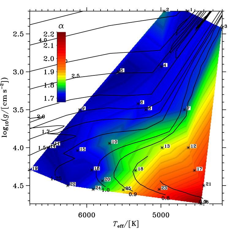
Figure 6: The mass mixing-length in units of $H_{P}$ for the 26 simulations, as listed in Table 1 in the $T_{\rm eff}$ – log g plane. We have also plotted evolutionary tracks (Schaller et al., 1992; Charbonnel et al., 1999) for masses as indicated at the bottom of each track.

4 Discussion and Summary

The basic structure of stellar convection zones is determined by the need to conserve mass. Stars are highly stratified so most of the mass ascending from depth must turn over and go back down within the order of a scale height. The high density mass from the interior can not be supported in the low density outer layers. This produces a true mixing by entrainment of the almost laminar upflows into the turbulent downflows. There is therefore a real physical basis for the mixing length theory of convection. From computational fluid dynamic simulations of stellar convection zones one can calculate this real mixing of mass to determine the length scale on which it occurs. Naively, one might expect it to be some multiple of the density scale height. However, as we observed for the Sun in Figure 3, it is actually the ratio of the mass mixing length to the pressure scale height which is nearly constant over many orders of magnitude change in the pressure. All of our values of mass mixing lengths are therefore presented in terms of the pressure scale height, $H_{P}$.

In Figure 6 we present the variation of $\alpha=\ell/H_{P}$ with the atmospheric parameters $T_{\rm eff}$ and $\log g$. First off, comparing the range of $\alpha$ with the uncertainties in Table 1, we see that the variation over the HR diagram is small, but significant. The range of values found here (1.6-2.2) is consistent with those used in stellar evolution calculations (Salaris & Cassisi, 2008; Montalbán & D’Antona, 2006; Montalbán et al., 2004; Fernandes et al., 1998; Chieffi et al., 1995; Pedersen et al., 1990), although such calculations assume a constant value for $\alpha$ as the star evolves. We have also compared the mass mixing length values found here with those determined by matching the adiabat in the convection zone from the simulations with that obtained from mixing length theory stellar models (Trampedach et al., 2011b). We find excellent agreement except for the coolest, low mass, dwarf stars where the mass mixing length values are larger. It should also be remembered that in addition to the other mixing length parameters specifying geometry and radiative energy exchange, other input physics, atmospheric opacities and the T-$\tau$ relation, also influence the appropriate value of the mixing length to use in stellar structure and evolution calculations.

We find $\alpha$ is smallest towards the high-$T_{\rm eff}$ and low-$g$ side of the diagram. These are also the simulations that have the least efficient convection, where high speeds and large superadiabatic gradients are necessary for carrying the flux to the photosphere. The least efficient convection has the smallest mass mixing lengths, as expected. The most efficient mixing occurs in the coolest dwarf with the most sedate convection. The solar value from our grid of simulations of $\alpha_{\odot}=1.76\pm 0.08$ agrees well with several determinations from the literature, lending credence to the solar models and to the common practice of calibrating $\alpha_{\rm MLT}$ against such models. We also see from Figure 6, however, that the solar value is less applicable for lower mass stars, which also have the largest change of $\alpha$ during their evolution. The evolution of higher-mass stars and the ascent up the Hayashi-track, seems well described by a single value of $\alpha$.

The surface layers cannot be properly accounted for with a MLT-like formulation. Crucial components like over-shooting, turbulent pressure, radiative transfer in the presence of large temperature inhomogeneities, etc., are not included in this simple model, but greatly affect the surface layers. The mass mixing length found here, is the appropriate mixing length to use in a formulation that can realistically include all these phenomena — an ideal MLT formulation. Still lacking such a formulation, the solar mass mixing length found in the present work, does not necessarily agree with that found from matching solar evolution models to the Sun’s present luminosity and radius. The latter furthermore depends on all the other ingredients going into the atmosphere of the evolution model, such as atmospheric opacities and how the photospheric transition from optically thick to optically thin is treated, e.g., through some match to an atmosphere model or through $T$-$\tau$ relations. The mixing length of MLT is strongly connected to the actual length-scale of mixing, as found in this paper, but this connection is weakened by all these confounding factors entering into the MLT version.

The increase in the ratio of mass mixing length to pressure scale height in the superadiabatic layers near the surface raises the question of why stellar evolution calculations with the interior values of $\alpha$ work well in matching observations of global stellar properties. In this regard, note that to match line profiles (e.g. Balmer lines ) a small value of $\alpha$ that produces a steep temperature gradient is needed in the atmosphere. In this case, a large value of $\alpha$ must be used in the interior (Montalbán et al., 2004). Our result suggest such a two value set of mixing length parameters may indeed be appropriate. However, the main conclusion should be that mixing length theory is not well defined and different variations are possible that will yield similar results.

Calculations, such as presented here, will reduce the uncertainty in the appropriate choice of mixing length in stellar structure and evolution calculations. In particular, we have used the behavior with depth, to discriminate between various mixing length formulations, and find that the mass mixing length, $\ell$, is best described with a constant $\alpha_{P}=\ell/H_{P}$. In a future paper (Trampedach et al., 2011b) we present calibrations of $\alpha_{P}({\rm MLT})$ against the simulations, based on 1D MLT envelope models that employ the exact same EOS and opacities as the simulations, and use a new self-consistent treatment of $T$-$\tau$ relations, computed from the simulations (Trampedach et al., 2011a). That calibration will be aimed at reproducing the asymptotic adiabat with a standard MLT formulation, and will contain our recommended values for $\alpha_{P}({\rm MLT})$. Our present calculation of $\alpha$ is model independent in that we compute the actual physical mixing length of the simulations, without connecting it to a particular MLT formulation. Our present result, that $\alpha_{P}$ seems convergent with depth, is a confirmation that MLT is a physically reasonable model for stellar convection, despite its many shortcomings, particularly near the surface. The present work also confirms the soundness of the scheme employed in the Trampedach et al. (2011b) $\alpha_{P}({\rm MLT})$ calibration, since, for most of the simulations, it results in $\alpha$-values very similar to what we find here. This agreement between the two independent methods, suggests that $\alpha_{P}({\rm MLT})$ has been approximately disentangled from the various uncertainties in atmospheric physics that have historically been absorbed into $\alpha_{\rm MLT}$.

With the results from Trampedach et al. (2011a, b), supported by our present results, 1D MLT models can be made more self-consistent and with a reduced set of free parameters. From an MLT point of view, there are of course still the undetermined geometric form factors that could conceivably be adjusted to match the adiabat in conjunction with the mass mixing length found here.

References

- Böhm-Vitense (1958) Böhm-Vitense, E. 1958, ZAp, 46, 108
- Canuto & Mazzitelli (1991) Canuto, V. M., & Mazzitelli, I. 1991, ApJ, 370, 295
- Charbonnel et al. (1999) Charbonnel, C., Däppen, W., Schaerer, D., Bernasconi, P. A., Maeder, A., Meynet, G., & Mowlavi, N. 1999, A&APS, 135, 405
- Chieffi et al. (1995) Chieffi, A., Straniero, O., & Salaris, M. 1995, ApJ, 445, L39
- Fernandes et al. (1998) Fernandes, J., Lebreton, Y., Baglin, A., & Morel, P. 1998, A&A, 338, 455
- Fernandes et al. (2002) Fernandes, J., Morel, P., & Lebreton, Y. 2002, A&A, 392, 529
- Ferraro et al. (2006) Ferraro, F. R., Valenti, E., Straniero, O., & Origlia, L. 2006, ApJ, 642, 225
- Freytag & Salaris (1999) Freytag, B., & Salaris, M. 1999, ApJ, 513, L49
- Gough (1977) Gough, D. O. 1977, in IAU Coll. 38, Lecture Notes in Physics, Vol. 71, Problems of stellar convection, ed. E. A. Spiegel & J. P. Zahn (Berlin: Springer), 15–56
- Gustafsson et al. (1975) Gustafsson, B., Bell, R. A., Eriksson, K., & Nordlund, Å. 1975, A&A, 42, 407
- Hummer & Mihalas (1988) Hummer, D. G., & Mihalas, D. 1988, ApJ, 331, 794
- Iben (1967) Iben, Jr., I. 1967, ARA&A, 5, 571
- Kurucz (1992) Kurucz, R. L. 1992, Rev. Mex. Astron. Astrofis., 23, 45
- Ludwig et al. (1999) Ludwig, H., Freytag, B., & Steffen, M. 1999, A&A, 346, 111
- Montalbán & D’Antona (2006) Montalbán, J., & D’Antona, F. 2006, MNRAS, 370, 1823
- Montalbán et al. (2004) Montalbán, J., D’Antona, F., Kupka, F., & Heiter, U. 2004, A&A, 416, 1081
- Nordlund (1976) Nordlund, A. 1976, A&A, 50, 23
- Pedersen et al. (1990) Pedersen, B. B., Vandenberg, D. A., & Irwin, A. W. 1990, ApJ, 352, 279
- Salaris & Cassisi (2008) Salaris, M., & Cassisi, S. 2008, A&A, 487, 1075
- Schaller et al. (1992) Schaller, G., Schaerer, D., Meynet, G., & Maeder, A. 1992, A&APS, 96, 269
- Stassun et al. (2004) Stassun, K. G., Mathieu, R. D., Vaz, L. P. R., Stroud, N., & Vrba, F. J. 2004, ApJS, 151, 357
- Stein et al. (2009) Stein, R. F., Georgobiani, D., Schafenberger, W., Nordlund, Å., & Benson, D. 2009, in Amer. Inst. of Phys. Conf. Ser., Vol. 1094, , 764–767
- Stein & Nordlund (1989) Stein, R. F., & Nordlund, Å. 1989, ApJ, 342, L95
- Stothers & Chin (1997) Stothers, R. B., & Chin, C. 1997, ApJ, 478, L103
- Trampedach et al. (2011a) Trampedach, R., Christensen-Dalsgaard, J., Nordlund, Å., Asplund, M., & Stein, R. F. 2011a, A&A, (submitted)
- Trampedach et al. (2011b) —. 2011b, (in preparation)
- Trampedach et al. (1999) Trampedach, R., Stein, R. F., Christensen-Dalsgaard, J., & Nordlund, Å. 1999, in Astron. Soc. Pac. Conf. Ser., Vol. 173, Stellar Structure: Theory and Test of Connective Energy Transport, ed. A. Gimenez, E. F. Guinan, & B. Montesinos, 233–236