Repeated Matching Pennies
with Limited Randomness

Abstract

We consider a repeated Matching Pennies game in which players have limited access to randomness. Playing the (unique) Nash equilibrium in this $n$-stage game requires $n$ random bits. Can there be Nash equilibria (or $\varepsilon$-Nash equilibria) that use less than $n$ random coins?

Our main results are as follows

• We give a full characterization of approximate equilibria, showing that, for any $\gamma\in[0,1]$, the game has a $\gamma$-Nash equilibrium if and only if both players have $(1-\gamma)n$ random coins.

• When players are bound to run in polynomial time with $n^{\delta}$ bits of randomness, approximate Nash equilibria can exist if and only if one-way functions exist.

• It is possible to trade-off randomness for running time. In particular, under reasonable assumptions, if we give one player only $O(\log n)$ random coins but allow him to run in arbitrary polynomial time with $n^{\delta}$ bits of randomness and we restrict his opponent to run in time $n^{k}$, for some fixed $k$, then we can sustain an $\varepsilon$-Nash equilibrium.

• When the game is played for an infinite amount of rounds with time discounted utilities, under reasonable assumptions, we can reduce the amount of randomness required to achieve a $\varepsilon$-Nash equilibrium to $n^{\delta}$, where $n$ is the number of random coins necessary to achieve an approximate Nash equilibrium in the general case.

1 Introduction

In the classical setting of Game Theory, one of the core assumptions is that all participating agents are “fully rational”. This amounts not only to the fact that an agent must be able to make optimal decisions, given the other players’ actions, but also to the fact that he must understand how these actions will affect the behavior of all other participants. If this is the case, a Nash equilibrium can be viewed as a set of strategies in which each agent is simply computing his best response given his opponents’ actions. However, in real world strategic interactions, people often behave in manners that are not fully rational. There are many reasons behind non-rational behavior, we focus on two: limitations on computation and limitations on randomness.

Since the work of Herbert Simon [13], much research has focused on defining models that take computational issues into account. In recent years, the idea that the full rationality assumption is often unrealistic has been formalized using tools and ideas from computational complexity. It is in fact easy to come up with settings, as in Fortnow and Santhanam [4], in which simply computing a best response strategy involves solving a computationally hard problem. Furthermore there is strong evidence that, in general, the problem of finding a Nash equilibrium is computationally difficult for matrix games (Daskalakis, Goldberg and Papadimitriou [3], Chen and Deng [2]).

Traditionally bounded rationality has focused on two computational resources: time and space. In this paper we focus on another fundamental resource: randomness.

It is a basic fact that games in which agents are not allowed to randomize might have no Nash equilibrium. In this sense, randomness is essential in game theory. We focus on a simple two player zero-sum game that captures this: Matching Pennies (Figure 1).

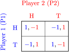
Figure 1: The payoff bimatrix for the Matching Pennies game.

Specifically, we consider the repeated version of Matching Pennies, played for $n$ rounds. In this game, the unique Nash equilibrium is the one in which, at every round, both players choose one of their two strategies uniformly at random. The algorithm that implements this strategy requires $n$ random coins, one for each round. The main question we address in this paper is: can there be Nash equilibria if the amount of randomness available to both players is less than $n$?

First we show that, in general, the game cannot have a Nash equilibrium in which both players have only a fraction of $n$ random coins. In particular, when we give both players $n(1-\gamma)$ random coins, we can only achieve a $\gamma$-Nash equilibrium. This turns out to be tight, in the sense that we can show that any game with a $\gamma$-Nash equilibrium both players must have at least $n(1-\gamma)$ coins.

The proof of this fact, however, relies on the players’ ability to implement a strategy that runs in exponential time. We then consider games in which the players’ strategies are polynomially-bounded. Using ideas developed in cryptography and computational complexity we show that, in this setting, $\varepsilon$-Nash equilibria that use only $n^{\delta}$ coins exist if and only if one-way functions exist.

We also show that the amount of randomness can be “traded” for time. If we allow one of the players to run in arbitrary polynomial time, but use only $O(\log n)$ bits, we can still achieve a $\varepsilon$-Nash equilibrium if we restrict his opponent to run in time $n^{k}$ for some fixed $k>0$, while giving him $n^{\delta}$ random bits.

Finally we consider an infinitely repeated game with time discounted utilities. In this case, in general, for any discount factor $\delta$ and approximation $\varepsilon$, we can always achieve a $\varepsilon$-Nash equilibrium with only $n$ random coins, if $n$ is large enough. When we limit players’ strategies to polynomial size circuits, we can reduce the amount of randomness to $n^{\delta}$, for any $\delta>0$.

Related Work

There are many recent approaches to bounded rationality using a computational complexity perspective. For instance Halpern and Pass [7] study games in which players’ strategies are Turing machines. The idea of considering randomness as a costly resource in game theory has received only limited attention. Kalyanaraman and Umans [11] study zero-sum games, and give both an efficient deterministic algorithm for finding $\varepsilon$-Nash equilibria, as well as a weaker, but more general, result in the spirit of our Lemma 3.1, giving a randomness-efficient adaptive on-line algorithm for playing repeated zero-sum games. Hu [9] also considers a similar setting but he is concerned with computability rather than complexity. He considers infinitely repeated plays of 2 player zero-sum games that have no pure strategy Nash equilibrium, and in which players have a set of feasible actions, which represents both the strategies they can play and the strategies they can predict. In this setting Hu gives necessary and sufficient conditions for the existence of Nash equilibria. Finally Gossner and Tomala [6], give entropy bounds on Bayesian learning in a game theoretic setting, in a more general framework then this paper. Their results applied to Matching Pennies do not achieve the tight bounds we get in Lemma 3.1.

The rest of the paper is organized as follows. In Section 2 we introduce the notation and known results used. Section 3 presents an information theoretic impossibility result. Section 4 considers players whose strategies are limited to polynomial sized Boolean circuit families, while Sections 5 and 6 give extensions of the main results to complexity pseudorandom number generators and infinitely repeated versions of the game.

2 Background and Definitions

2.1 Game Theory Notation

Throughout the paper we consider a repeated game of Matching Pennies. We focus on this game because it captures one of the fundamental aspects of randomness in game theory. Studying such a simple game also allows us to get tight bounds. However, variations of our results extend to other similar 2 person zero-sum repeated games.

The payoffs at each round are shown in Figure 1. Let $h:\{\text{H,T}\}\times\{\text{H,T}\}\to\{-1,1\}$, be the payoff to Player 1 (P1), and $-h$ the payoff for P2. When we allow the players to randomize, we denote as $S_{i}$ a randomized strategy on $\Delta\{H,T\}$ for player $i$. P1’s expected payoff in one round is

$$\mathbf{E}\left[h(S_{1},S_{2})\right]=\sum_{s_{1},s_{2}\in\{\text{H,T}\}}\text{Pr}\left(S_{1}=s_{1}\right)\text{Pr}\left(S_{2}=s_{2}\right)h(s_{1},s_{2}).$$

Let $u:\{\text{H,T\}}^{n}\times\{\text{H,T\}}^{n}\to\{-n,\cdots,n\}$ be P1’s cumulative payoff when the game is played for $n$ rounds. In the repeated game, mixed strategies can be viewed as distribution over sequences of length $n$ that are dependend on the opponent’s strategy. Given the adversary’s strategy, let $R_{i}=(r_{i}^{1},\cdots,r_{i}^{n})\in\Delta\{\text{H,T\}}^{n}$ denote a randomized strategies for player $i$. P1’s expected cumulative payoff is

$$\mathbf{E}\left[u(R_{1},R_{2})\right]=\sum_{t=1}^{n}\mathbf{E}\left[h(r_{1}^{t},r_{2}^{t})\right].$$

Finally we define the expected average payoff to P1 for the $n$-round game as

$$\mathbf{E}\left[U(R_{1},R_{2})\right]=\frac{\mathbf{E}\left[u(R_{1},R_{2})\right]}{n},$$

and consequently P2’s expected payoff is $-\mathbf{E}\left[U(R_{1},R_{2})\right]$. To denote player’s $i$ payoff we will sometimes use the standard notation $\mathbf{E}\left[U(R_{i},R_{-i})\right]$, where $R_{i}$ is player’s $i$ mixed strategy and $R_{-i}$ is his opponent’s mixed strategy.

Definition 2.1 (Nash equilibrium).

A pair of mixed strategies $(R_{1},R_{2})$ is a Nash equilibrium for the $n$-stage Matching Pennies game if, for $i=1,2$:

$$\mathbf{E}\left[U(R_{i},R_{-i})\right]\geq\mathbf{E}\left[U(R_{i}^{\prime},R_{-i})\right]\quad\text{for all }R_{i}^{\prime}\in\Delta\{\text{H,T}\}^{n}.$$

In some cases we will consider a relaxed notion of equilibrium, namely $\varepsilon$-Nash equilibrium.

Definition 2.2 ($\varepsilon$-Nash equilibrium).

A pair of mixed strategies $(R_{1},R_{2})$ is a $\varepsilon$-Nash equilibrium for the $n$-stage Matching Pennies game if, for $i=1,2$:

$$\mathbf{E}\left[U(R_{i},R_{-i})\right]\geq\mathbf{E}\left[U(R_{i}^{\prime},R_{-i})\right]-\varepsilon\quad\text{for all }R_{i}^{\prime}\in\Delta\{\text{H,T}\}^{n}.$$

2.2 Complexity and Pseudorandomness

We give a brief description of the pseudorandomness tools we need for this paper. For more details we recommend the textbooks of Arora and Barak [1] and Goldreich [5].

The model of computation used throughout most of the paper is based on Boolean Circuits. We consider circuits with AND, OR and NOT gates, and denote by $C_{n}$ a circuit with $n$ input nodes. A circuit family $\{C_{i}\}_{i\in\mathbb{N}}$ is an infinite collection of circuits, intuitively one for each input length.

The size of a circuit $|C_{n}|$ is the number of gates. A circuit family is polynomial sized if there is a $k>0$ such that, for all $n$, $|C_{n}|\leq n^{k}$. The class of languages recognizable by families of polynomial sized circuits is called P/Poly. Any language that can be decided in polynomial time by a deterministic or randomized Turing machine is also in P/Poly. Formally $\textsf{P}\subseteq\textsf{BPP}\subseteq\textsf{P/Poly}$.

A function is one-way if it is easy to compute and hard to invert.

Definition 2.3 (One-way Function).

A one-way function is a polynomial-time computable function $f:\{0,1\}^{n}\to\{0,1\}^{n}$ such that, for all polynomial size circuits $D$ and $y=f(x)$ (where $x$ is chosen uniformly at random on $\{0,1\}^{n}$), $\Pr(f(D(y))=f(x))<n^{-c}$ for all $c>0$ and sufficiently large $n$.

Informally, two objects are indistinguishable if no polynomial sized circuit family can tell them apart with noticeable probability.

Definition 2.4 (Indistinguishability).

Let $X,Y$ be two random variables on $\{0,1\}^{n}$. We say that $X$ and $Y$ are computationally indistinguishable if for every family of polynomial size circuits $\left\{C_{i}\right\}_{i\in\mathbb{N}}$, every $c>0$ and for sufficiently large $n$

$$\Big{|}\text{Pr}\left(C_{n}\left(X\right)=1\right)-\text{Pr}\left(C_{n}\left(Y\right)=1\right)\Big{|}<\frac{1}{n^{c}}.$$

A cryptographic pseudorandom number generator (PRNG) is a deterministic algorithm whose output is computationally indistinguishable from the uniform distribution, provided that it’s input is truly random. We will denote by $U_{k}$ a random variable uniformly distributed on $\{0,1\}^{k}$.

Definition 2.5 (Cryptographic PRNG).

A cryptographic pseudorandom number generator is a deterministic polynomial time algorithm $G:\{0,1\}^{l(n)}\to\{0,1\}^{n}$, where $l(n)<n$ is a polynomial time computable function, such that $G(U_{l(n)})$ and $U_{n}$ are computationally indistinguishable.

There are two basic properties about pseudorandom number generators that we will use. One relates the notion of pseudorandomness to the notion of predictability.

Definition 2.6 (Unpredictable).

Let $G:\{0,1\}^{l(n)}\to\{0,1\}^{n}$ be a polynomial time algorithm, and $G(x)=(y_{1},\cdots,y_{n})$. We call $G$ unpredictable if for every family of polynomial size circuits $\left\{D_{i}\right\}_{i\in\mathbb{N}}$, all $c>0$ and for sufficiently large $n$

$$\text{Pr}\left(D_{i}\left(y_{1},\dots,y_{i-1}\right)=y_{i}\right)\leq\frac{1}{2}+\frac{1}{n^{c}}.$$

Intuitively a pseudorandom number generator must be unpredictable, otherwise we could easily build a test for it by using the predictor circuits. In 1982 Yao [14] proved the opposite implication, thus establishing the following theorem.

Theorem 2.7 (Yao’s Theorem).

A polynomial time algorithm $G:\{0,1\}^{l(n)}\to\{0,1\}^{n}$ is unpredictable if and only if $G$ is a pseudorandom number generator.

Håstad, Impagliazzo, Luby and Levin in 1999 [8] showed how to construct pseudorandom number generators with polynomial expansion based on one-way functions.

Theorem 2.8 (PRNG’s from one-way functions).

One way functions exist if and only if for every $\delta>0$ there is a pseudorandom number generator with $l(n)=n^{\delta}$.

Cryptographic pseudorandom number generators’ main power lies in the ability to fool any polynomial sized adversary, while running in polynomial time. However, in other areas of complexity, such as derandomization, the crucial issue is having a smaller seed.

Definition 2.9 (Complexity PRNG).

A complexity pseudorandom number generator is a $2^{l(n)}$ time computable function $G:\{0,1\}^{l(n)}\to\{0,1\}^{n}$, such that for any circuit $C$ of size $n$

$$\Big{|}\text{Pr}\left(C\left(U_{l(n)}\right)=1\right)-\text{Pr}\left(C\left(G\left(U_{n}\right)\right)=1\right)\Big{|}<n^{-1}.$$

The essential difference with cryptographic pseudorandom number generators is the order of quantifiers. A cryptographic pseudorandom number generator fools circuits of an arbitrary polynomial size. The complexity pseudorandom number generator fools circuits only of a fixed polynomial size but under the right assumptions requires far fewer random bits.

Impagliazzo and Wigderson [10] building on a series of paper starting with Nisan and Wigderson [12] characterize when complexity pseudorandom number generators exist.

Theorem 2.10.

There exists $L\in\textsf{DTIME}(2^{O(l(n))})$ and $\varepsilon>0$ such that no circuit of size at most $2^{\varepsilon l(n)}$ can compute $L$ if and only if there exists a complexity pseudorandom number generator with $l(n)=C\log n$ for some $C>0$.

3 Information Theoretic Bounds

In this section we make no computational assumptions on the players, and show that there can be no Nash equilibrium if we limit the amount of randomness available to both players.

Lemma 3.1.

For any $\gamma\in[0,1]$, if P2 has less than $n(1-\gamma)$ random bits, then P1 has a deterministic strategy $A$ that achieves an expected average payoff of at least $\gamma$.

Proof.

We will give a strategy $A=(a^{1},\cdots,a^{n})$ for P1 that achieves a high payoff against any strategy $B=(b^{1},\cdots,b^{n})$ from P2.

Player 1 will enumerate all of P2’s possible coin flips, and will obtain a set of $2^{n(1-\gamma)}$ possible strategies, one of which is the one being used by P2. After each play by P2, P1 can eliminate all the strategies that do not play that action at that round. Let $S^{t}$ be the set of strategies that are consistent with P2’s plays up to round $t$. Initially the set $S^{1}$ contains $2^{n(1-\gamma)}$ strategies, and, for all $t$, $|S^{t+1}|\leq|S^{t}|$.

The strategy $A$ for P1 is straightforward: at round $t$, P1 will play based on the most likely event: he will consider all strategies in $S^{t}$ and play H if the majority of strategies in $S^{t}$ use H at round $t$ and play T otherwise. Let $p^{t}$ be the exact fraction of strategies that are the majority at round $t$,

$$p^{t}=\frac{\max\{|\{b^{t}~{}|~{}b^{t}=H\}|,|\{b^{t}~{}|~{}b^{t}=T\}|\}}{|S^{t}|},$$ (3.1)

so that $p^{t}\in[1/2,1]$. P1’s expected payoff at round $t$ is:

$$\mathbf{E}\left[h(a^{t},b^{t})\right]=p^{t}-(1-p^{t})=2p^{t}-1\geq 0.$$

Thus P1’s average expected payoff is at least 0. To show that P1 can actually achieve an average expected payoff of $\gamma$ we need to consider the amount of information P1 gains at each round. We define the following potential function $\phi:\{1,\dots,n\}\to\mathbb{R}$:

$$\phi(t)=\sum_{k=1}^{t-1}h(a^{k},b^{k})-\log|S^{t}|,$$

which considers both the accumulated payoff for P1 and the log-size of the set of consistent strategies. At time $t=1$ there are $2^{n(1-\gamma)}$ possible strategies for P2, so $\phi(1)=-n(1-\gamma)$. We will now lower bound the expected increase in $\phi$ at each round. We can express this as

$$\mathbf{E}\left[\phi(t+1)-\phi(t)\right] =\left(\mathbf{E}\left[\sum_{k=1}^{t}h(a^{k},b^{k})\right]-\mathbf{E}\left[\sum_{k=1}^{t-1}h(a^{k},b^{k})\right]\right)$$

$$\qquad\qquad-\left(\mathbf{E}\left[\log|S^{t+1}|\right]-\mathbf{E}\left[\log|S^{t}|\right]\right)$$

$$=\mathbf{E}\left[h(a^{t},b^{t})\right]-\left(\mathbf{E}\left[\log|S^{t+1}|-\log|S^{t}|\right]\right)$$

$$=2p^{t}-1-\left(\mathbf{E}\left[\log|S^{t+1}|-\log|S^{t}|\right]\right).$$

Now consider $\mathbf{E}\left[\log|S^{t+1}|\right]$. When P1 looses he can eliminate a $p^{t}$ fraction of strategies, thus the new set $S^{t+1}$ will contain a $(1-p^{t})$ fraction of the strategies in $S^{t}$. On the other hand, when P1 wins, $|S^{t+1}|=p^{t}|S^{t}|$. To complete the analysis we have to consider two cases, since if $p^{t}=1$ then $\mathbf{E}\left[\log|S^{t+1}|\right]$ is not well defined.

First assume $p^{t}=1$. This happens when all feasible strategies for P2 have the same action at round $t$. In this case P1 will win with probability 1, and the size of the set of feasible strategies will stay the same. So, overall, the increase in $\phi$ will be 1.

Now assume $p^{t}\in[1/2,1)$. Then, the expected size of the set $S^{t+1}$ is:

$$\mathbf{E}\left[\log|S^{t+1}|\right]=\left((1-p^{t})\log(1-p^{t})|S^{t}|+p^{t}\log p^{t}|S^{t}|\right).$$ (3.2)

The expected change in $\log|S^{t}|$ does not depend on $S^{t}$, but only on $p^{t}$, since

$$\mathbf{E}\left[\log|S^{t+1}|-\log|S^{t}|\right] =\left[(1-p^{t})\log(1-p^{t})|S^{t}|\right.$$

$$\left.\quad\qquad+p^{t}\log p^{t}|S^{t}|\right]-\log|S^{t}|$$

$$=(1-p^{t})\log(1-p^{t})+p^{t}\log p^{t}.$$

So that the overall change in potential when $p^{t}<1$ is

$$\mathbf{E}\left[\phi(t+1)-\phi(t)\right]\geq 2p^{t}-1-(1-p^{t})\log(1-p^{t})-p^{t}\log p^{t},$$

which is always at least $1$ for $p^{t}\geq 1/2$.

So, for all $p^{t}\in[1/2,1]$, at each step the potential function $\varphi$ increases by at least $1$. Thus, after $n$ rounds we have that

$$\mathbf{E}\left[\phi(n)\right] \geq\phi(1)+\min_{t}\{n\mathbf{E}\left[\phi(t+1)-\phi(t)\right]\}$$

$$\geq-n(1-\gamma)+n=n\gamma.$$

Since P1’s expected payoff is at least $\mathbf{E}\left[\phi(n)\right]$, this completes the proof. ∎

This result immediately implies that, without any computational assumption, there can be no equilibrium with less than $n$ random coins.

Corollary 3.2.

For all $\gamma_{1},\gamma_{2}\in[0,1]$ such that $\gamma_{1}+\gamma_{2}>0$, if P1 and P2 have, respectively, $n(1-\gamma_{1})$ and $n(1-\gamma_{2})$ random coins, then there can be no Nash equilibrium in the $n$-stage Matching Pennies repeated game.

Proof.

Assume, by contradiction, that $(S_{1},S_{2})$ is such a Nash equilibrium. By Lemma 3.1, P1’s expected payoff must be $\mathbf{E}\left[U(S_{1},S_{2})\right]\geq\gamma_{2}$ and P2’s payoff $-\mathbf{E}\left[U(S_{1},S_{2})\right]\geq\gamma_{1}$, otherwise they would be better off by using the majority strategy in the proof of Lemma 3.1. Summing the two inequalities we get $\gamma_{1}+\gamma_{2}\leq 0$, a contradiction, since we assume $\gamma_{1}+\gamma_{2}>0$. ∎

However, if we limit the amount of randomness available to both players, we are still able to achieve an $\varepsilon$-Nash equilibrium. Furthermore, if the game has a $\varepsilon$-Nash equilibrium, then both players must have at least $(1-\varepsilon)n$ random coins.

Theorem 3.3.

Let $\gamma\in[0,1]$. The game has a $\gamma$-Nash equilibrium if and only if both players have $n(1-\gamma)$ random coins.

For simplicity we assume $\gamma$ is the same for both players, however a similar result holds even in the case where the two players have a different amount of random coins.

Proof.

To show the “only-if” implication, consider, by way of contradiction, a game that has a $\gamma$-Nash equilibrium $(S_{1},S_{2})$ but in which both players have less than $n(1-\gamma)$ random bits. Thus there must be a $\gamma^{\prime}>\gamma$ such that they have exactly $n(1-\gamma^{\prime})$ random bits. Since $(S_{1},S_{2})$ is a $\gamma$-Nash equilibrium, it must be the case that, for any strategy $S_{1}^{\prime}$ for P1

$$\mathbf{E}\left[U(S_{1},S_{2})\right]\geq\mathbf{E}\left[U(S_{1}^{\prime},S_{2})\right]-\gamma.$$

By Lemma 3.1 we know that both players have a strategy that achieves a payoff of at least $\gamma^{\prime}>\gamma$, so that the above implies $\mathbf{E}\left[U(S_{1},S_{2})\right]>0$. Applying the same argument to P2, we get $-\mathbf{E}\left[U(S_{1},S_{2})\right]>0$, a contradiction.

The “if” part follows from Lemma 3.4 below. ∎

Lemma 3.4.

Let $\gamma\in[0,1]$. If both players have $n(1-\gamma)$ random coins, then the game has a $\gamma$-Nash equilibrium.

For simplicity we assume $\gamma n$ is even.

Proof.

Consider the following strategies: both player use their random coins to play uniformly at random for the first $n(1-\gamma)$ rounds. Thereafter P1 will always play $H$, while P2 will alternate between $H$ and $T$, playing $H,T,\dots$. We claim that this is a $\gamma$-Nash equilibrium.

First notice that no player can improve his payoff in the first $n(1-\gamma)$ rounds, given his opponent’s strategy. Let’s consider the remaining $n\gamma$ rounds. P1 could improve his payoff by playing $H,T,H,T\dots$, however this only increases his payoff by $\gamma$. This holds also for P2, that could play $T,T,\dots$, however gaining only $\gamma$. ∎

4 Computationally Efficient Players

The proof of Lemma 3.1 in the previous section relies heavily the fact that we make no computational assumptions. In particular, to implement the majority strategy and compute $p^{t}$ in (3.1) requires solving $\#$P hard problems, by reduction from $\#$SAT. If we restrict the players to run in time polynomial in $n$ this particular strategy likely becomes unfeasible. In this setting, under reasonable complexity assumptions, it is possible to greatly reduce the amount of randomness and, at the same time, achieve a $\varepsilon$-Nash equilibrium.

We consider players’ whose actions are polynomial size Boolean circuits. A strategy is thus a circuit family $\{C_{i}\}_{i\in\mathbb{N}}$, such that circuit $C_{l(n)}$ takes as input $l(n)$ random coins and outputs the $n$ actions to be played. Notice that this definition implies that each agent can simulate any of his opponent’s strategies.

We consider equilibria that use $n^{\delta}$ random coins for any $\delta>0$. Theorem 4.1 shows that such $\varepsilon$-Nash equilibria exist if and only if one-way functions exist.

Theorem 4.1.

If players are bound to run in time polynomial in $n$, then, for all $\delta>0$ and sufficiently large $n$, $\varepsilon$-Nash equilibria that use only $n^{\delta}$ random coins exist, where $\varepsilon=n^{-k}$ for all $k>0$ and sufficiently large $n$’s, if and only if one-way functions exist.

Proof.

The if part is Lemma 4.3, while the only-if part is Lemma 4.4. ∎

As a preliminary result we show that, in our setting, the expected utility when at least one player uses a pseudorandom number generator can’t be too far from the expected utility when playing uniformly at random.

Lemma 4.2.

Assume one-way functions exist, and let $G$ be the strategy corresponding to the output of a pseudorandom number generator. For any strategy $S$ that runs in time polynomial in $n$, for all $k>0$ and sufficiently large $n$,

$$\Big{|}\mathbf{E}\left[U(G,S)\right]\Big{|}\leq n^{-k}\text{ and }\Big{|}\mathbf{E}\left[U(S,G)\right]\Big{|}\leq n^{-k}.$$

Proof.

We prove only the first inequality, the proof for the second one being symmetric.

Proof by contradiction. Assuming there is a $k>0$ such that $\Big{|}\mathbf{E}\left[U(G,S)\right]\Big{|}>n^{-k}$ for infinitely many $n$’s, we will construct a test $T$ for $G$, and show that

$$\Big{|}\text{Pr}\left(T\left(G\left(U_{l(n)}\right)\right)=1\right)-\text{Pr}\left(T\left(U_{n}\right)=1\right)\Big{|}>n^{-c}$$ (4.1)

for some $c>0$ and infinitely many $n$’s, thus contradicting the assumption that $G$ is a pseudorandom number generator.

First consider the $n$ random variables $A_{i}(G,S)$, for $i=1,\cdots,n$, where $A_{i}(G,S)$ is simply P1’s payoff at round $i$. Since $\sum_{i=1}^{n}A_{i}(G,S)=nU(G,S)$,

$$\sum_{i=1}^{n}\mathbf{E}\left[A_{i}(G,S)\right]>n^{1-k}.$$

This implies that there must be an $i$ such that $\mathbf{E}\left[A_{i}(G,S)\right]>n^{-k}$. Fix that $i$.

The test $T$ takes as input an $n$-bit sequence $x$ and generates a sequence of plays $s$ according to strategy $S$. Now $T$ simulates an $n$-stage repeated Matching Pennies game with strategies $(x,s)$. If P1 wins the $i$-th round then it will output 1, otherwise the output will be 0. In other words, $T$ outputs 1 if and only if $A_{i}(x,s)=1$. Notice that $T$ runs in time polynomial in $n$.

When $x$ is drawn from the uniform distribution, P1 will win with probability $1/2$, or $\text{Pr}\left(T(U_{n})=1\right)=1/2$.

Now notice, that since $A_{i}\in\{-1,1\}$, $\text{Pr}\left(A_{i}=1\right)=\frac{\mathbf{E}\left[A_{i}\right]+1}{2}$. This implies that

$$\text{Pr}\left(T(G(U_{l(n)}))=1\right)=\frac{\mathbf{E}\left[A_{i}\right]+1}{2}>\frac{1}{2n^{k}}+\frac{1}{2}.$$

Thus

$$\Big{|}\text{Pr}\left(T\left(G_{1}\left(U_{l(n)}\right)\right)=1\right)-\text{Pr}\left(T\left(U_{n}\right)=1\right)\Big{|}>\frac{1}{2n^{k}},$$

which proves the lemma. ∎

Lemma 4.3.

If one-way functions exist and players are bound to run in time polynomial in $n$, then for every $\delta,k>0$ and for sufficiently large $n$, the $n$-stage has an $n^{-k}$-Nash equilibrium in which each player uses at most $n^{\delta}$ random bits.

Proof.

Assume, by contradiction, that one-way functions exist but there are values $\delta>0$ and $k>0$ such that the game has no $n^{-k}$-Nash equilibrium in which players use at most $n^{\delta}$ random coins.

Since we assume one-way functions exist, by Theorem 2.8 there exist pseudorandom number generators that use $n^{\delta}$ coins. Assume both players use the output of such pseudorandom number generators as their strategies (which we call, respectively, $G_{1}$ and $G_{2}$). Since we are assuming that this is not a $n^{-k}$-Nash equilibrium, one of the players, say Player 1, must have a strategy $A$ such that

$$\mathbf{E}\left[U\left(A,G_{2}\right)\right]>\mathbf{E}\left[U\left(G_{1},G_{2}\right)\right]+n^{-k}.$$ (4.2)

By Lemma 4.2 we can choose a $k^{\prime}>0$ such that

$$\mathbf{E}\left[U\left(A,G_{2}\right)\right]>-n^{-k^{\prime}}+n^{-k}.$$ (4.3)

Pick $c=k^{\prime}=k+1$, so that $\mathbf{E}\left[U\left(A,G_{2}\right)\right]>n^{-c}$ for $n>2$. This contradicts Lemma 4.2, proving the claim. ∎

We now prove the opposite direction, that is that the existence of Nash equilibria that use few random bits implies the existence of one-way functions.

Lemma 4.4.

If for every $\delta>0$ there is a Nash equilibrium in which each player uses $n^{\delta}$ random bits and runs in time polynomial in $n$, then one-way functions exist.

Proof.

Let $(A,B)$ be such a Nash equilibrium and assume, by contradiction, that one-way functions don’t exist. This implies that pseudorandom number generators can’t exist (Goldreich [5]), and so, $A$ and $B$ can’t be sequences that are computationally indistinguishable from uniform.

Thus, by Yao’s theorem (Theorem 2.7), we know that there are polynomial size circuit families $\left\{C_{i}\right\}_{i\in\mathbb{N}}$ and $\left\{D_{i}\right\}_{i\in\mathbb{N}}$ such that

$$\text{Pr}\left(C_{i}(y_{1},\dots,y_{i})=y_{i+1}\right) >1/2+\delta_{1}$$

$$\text{Pr}\left(D_{i}(z_{1},\dots,z_{i})=z_{i+1}\right) >1/2+\delta_{2},$$

for some $\delta_{1},\delta_{2}>0$, where $A(x_{1},\dots,x_{l_{1}(n)})=(y_{1},y_{2},\dots,y_{n})$ and $B(x_{1},\dots,x_{l_{2}(n)})=(z_{1},z_{2},\dots,z_{n})$.

To get a contradiction it is sufficient to show that players are better off by using the predictor circuits $C$ and $D$. Consider Player 1: using $D$, at each round he can guess, given the previous history, the opponent’s next move with probability $\frac{1}{2}+\delta_{1}$. Thus his expected payoff at any round $t$ is

$$\mathbf{E}\left[h(d^{t},b^{t})\right]>\frac{1}{2}+\delta_{1}-\frac{1}{2}+\delta_{1}=2\delta_{1},$$

where the expectation is over the internal coin tosses of the predictor circuit $D$. The overall expected payoff is

$$\mathbf{E}\left[U(D,B)\right]>\frac{1}{n}\sum_{t=1}^{n}2\delta=2\delta_{1}.$$

Now, let $w=\mathbf{E}\left[U(A,B)\right]$ be the value of the expected payoff when players play $(A,B)$. Consider the following cases:

1. $w\leq 0$: this implies that Player 1 could gain $2\delta_{1}$ by using strategy $D$,

2. $w>0$: by definition Player 2’s expected payoff is $-\mathbf{E}\left[U(A,B)\right]<0$, so Player 2 can achieve a higher payoff by using his predictor circuit $C$,

In both cases we see that $(A,B)$ can’t be a Nash equilibrium, a contradiction. ∎

5 Exchanging Time for Randomness

In this section we determine conditions under which a $\varepsilon$-Nash equilibrium can arise, given that one of the players has only a logarithmic amount of randomness and his opponent must run in time $n^{k}$ for some fixed $k$. This shows how we can trade off randomness for time; the player with $O(\log n)$ random bits runs in time polynomial in $n$, while the player with more random bits runs in fixed polynomial time.

Theorem 5.1.

Assume there exists $f\in\textsf{DTIME}(2^{O(l(n))})$ and $\varepsilon>0$ such that no circuit of size at most $2^{\varepsilon l(n)}$ can compute $f$ and that one-way functions exist. Let Player 1’s strategies be circuits of size at most $n^{k}$ that use at most $n^{\delta}$ random bits for some $k>2+c\delta$, where $c\geq 1$ is a constant related to the implementation of a cryptographic pseudorandom number generator. Assume Player 2 has access to only $M\log n$ random bits. As long as $M>Ck$, where $C$ is the constant in Theorem 2.10, then for all $\varepsilon>0$ and sufficiently large $n$ there is a $\varepsilon$-Nash equilibrium.

Proof.

Let $G_{1}$ be the cryptographic pseudorandom number generator available to Player 1 and $G_{2}$ be the complexity pseudorandom number generator used by player 2. Furthermore let $\mathcal{S}_{1}$ be the set of all possible strategies for P1 (for all $\delta>0$ circuits of size at most $n^{k}$ that use $n^{\delta}$ random bits), and $\mathcal{S}_{2}$ the set of strategies available to P2 (polynomial size circuit families and $M\log n$ random coins). We will show that for all $\varepsilon>0$ and sufficiently large $n$, $(G_{1},G_{2})$ is a $\varepsilon$-Nash equilibrium with the required properties.

First we argue that, for all $\gamma>0$ and sufficiently large $n$, $|\mathbf{E}\left[U(G_{1},G_{2})\right]|<\gamma$. The proof of this fact is similar to the proof of Lemma 4.2, showing by way of contradiction, that if $|\mathbf{E}\left[U(G_{1},G_{2})\right]|\geq\gamma$ then we can build a test for the cryptographic pseudorandom number generator $G_{1}$.

Now we show that, for the appropriate setting of parameters, $G_{1}$ fools $\mathcal{S}_{2}$ and $G_{2}$ fools $\mathcal{S}_{1}$. For any $k$, Player 2 can fool circuits of size $n^{k}$ by using $C\log n^{k}=Ck\log n$ random bits. So, for $M>Ck$, $G_{2}$ fools $\mathcal{S}_{1}$. Notice also that since Player 2 runs in time $O(n^{Ck})$, the cryptographic pseudorandom number generator $G_{1}$ fools $\mathcal{S}_{2}$. Let $h$ be the one-way permutation used by the pseudorandom number generator $G_{1}$, and assume $h$ us computable in time $n^{c}$ for some $c>0$. Given $h$, $G_{1}$ is defined as follows: let $x,y\in\{0,1\}^{\frac{n^{\delta}}{2}}$, and let $(x,y)$ be $G_{1}$’s seed (notice that $|(x,y)|=n^{\delta}$), then

$$G_{1}(x,y)=\left(f^{n}(x)\odot y,f^{n-1}(x)\odot y,\dots,f(x)\odot y\right),$$

where $x\odot y=\sum_{i}x_{i}y_{i}\mod 2$. There are $O(n^{2})$ applications of $h$, so $G_{1}$ runs in time $O(n^{2+c\delta})$. So, for $k\geq 2+c\delta$, $G_{1}$ fools $\mathcal{S}_{2}$.

At this point we’re almost done. As in Lemma 4.3 assume, by contradiction, that the assumptions in the theorem hold but $(G_{1},G_{2})$ is not a $\varepsilon$-Nash equilibrium for some $\varepsilon>0$. This implies that at least one of the two players can improve his expected payoff by more than $\varepsilon$ by switching to some other strategy. First consider P2, and assume there is a strategy $S_{2}\in\mathcal{S}_{2}$ such that

$$\mathbf{E}\left[U(G_{1},S_{2})\right]>\mathbf{E}\left[U(G_{1},G_{2})\right]+\varepsilon.$$

As in Lemma 4.3 this implies that $S_{2}$ would be a test for the cryptographic pseudorandom number generator $G_{1}$, contradicting the fact that $G_{1}$ fools $\mathcal{S}_{2}$. Similarly, assume P1 has a strategy $S_{1}\in\mathcal{S}_{1}$ such that

$$\mathbf{E}\left[U(S_{1},G_{2})\right]>\mathbf{E}\left[U(G_{1},G_{2})\right]+\varepsilon.$$

Again, $S_{1}$ can easily be made into a test for $G_{2}$, contradicting the fact that $G_{2}$ fools $\mathcal{S}_{1}$. ∎

6 Infinite Play

We now consider an infinitely repeated game of Matching Pennies, and show that, if utilities are time discounted, we can always achieve a $\varepsilon$-Nash equilibria using a large enough (but finite) amount of random coins. First we determine the least amount of randomness required to achieve a $\varepsilon$-Nash equilibrium in the general, i.e. computationally unbounded, case.

Lemma 6.1.

For all discount factors $\delta\in(0,1)$ and all $\varepsilon>0$, there is an $\varepsilon$-Nash equilibrium in which the players use only $n$ random bits, for $n>\frac{\log\varepsilon(1-\delta)}{\log\delta}$.

Proof.

Given $\delta,\varepsilon>0$ consider the following strategies: both players play the Nash equilibrium strategy for the first $n$ rounds. After this P1 will always play $H$, while P2 will play $H$ and $T$ alternatively. The overall expected payoff is 0. However, after round $n$, both players could switch to a strategy that always wins, achieving a total expected payoff of $0+\sum_{t=n}^{\infty}\delta^{t}=\frac{\delta^{n}}{1-\delta}$. To ensure that our strategies are indeed a $\varepsilon$-Nash equilibrium we just need to make sure that

$$0>\frac{\delta^{n}}{1-\delta}-\varepsilon.$$

Rearranging and taking logarithms we get $n>\frac{\log\varepsilon(1-\delta)}{\log\delta}$. ∎

Now we consider players’ whose strategies are families of polynomial size Boolean circuits (as in Section 4), and assume one-way functions exist. We first give a version of Lemma 4.2 for time discounted utilities on a finite number of rounds.

Lemma 6.2.

Assume one-way functions exist, and let $G=(g^{1},\dots,g^{n})$ be the strategy corresponding to the output of a cryptographic pseudorandom number generator. Let $S=(s^{1},\dots,s^{n})$ be any strategy. For all $\delta\in(0,1)$, $k>0$ and for sufficiently large $n$

$$\Big{|}\mathbf{E}\left[\sum_{t=1}^{n}\delta^{t}h(g^{t},s^{t})\right]\Big{|}\leq n^{-k}\text{ and }\Big{|}\mathbf{E}\left[\sum_{t=1}^{n}\delta^{t}h(s^{t},g^{t})\right]\Big{|}\leq n^{-k}.$$

Proof.

Again we give the proof only for the first inequality. Assume, by contradiction, that $|\mathbf{E}\left[\sum_{t=1}^{n}\delta^{t}h(g^{t},s^{t})\right]|>n^{-k}$ for some $\delta$, $k$ and infinitely many $n$’s. Consider the random variables $A_{1}(c_{1}^{1},c_{2}^{1}),\dots,A_{n}(c_{1}^{n},c_{2}^{n})$, defined as $A_{t}(c_{1}^{t},c_{2}^{t})=1$ if P1 wins round $t$ when playing according to $(C_{1},C_{2})$ and 0 otherwise. Let $A(C_{1},C_{2})=\sum_{t}\delta^{t}A_{t}(c_{1}^{t},c_{2}^{t})$, so that $\mathbf{E}\left[A(G,S)\right]\geq|\mathbf{E}\left[\sum_{t=1}^{n}\delta^{t}h(g^{t},s^{t})\right]|>n^{-k}$. This implies that there is a $t$ such that $\delta^{t}\mathbf{E}\left[A_{t}(g^{t},s^{t})\right]>n^{-k-1}$, which implies $\mathbf{E}\left[A_{t}(g^{t},s^{t})\right]>n^{-k-1}$. Fix that $t$. As in Lemma 4.2, consider the test $T$ that, given a sequence of plays $x$, generates a play $s$ from $S$ and outputs 1 if P1 wins round $t$ and outputs 0 otherwise.

When $x$ is drawn uniformly at random, $\text{Pr}\left(T(U_{n})=1\right)=1/2$. On the other hand, when $x$ is $G$’s output,

$$\text{Pr}\left(T(G(U_{l(n)}))=1\right)=\mathbf{E}\left[A_{t}\right]>n^{-k-1}.$$

Now

$$\Big{|}\text{Pr}\left(T(G(U_{l(n)}))=1\right)-\text{Pr}\left(T(U_{n})=1\right)\Big{|}>\frac{1}{2}-\frac{1}{n^{k+1}}=\frac{1}{n^{c}},$$

for $c>-\frac{\log(1/2-n^{-1-k})}{\log n}\geq 0$, contradicting the assumption that $G$ is a pseudorandom number generator. ∎

Using the above Lemma we can show that, for all discount factors, we can greatly reduce the amount of random coins needed to get an $\varepsilon$-Nash equilibrium.

Lemma 6.3.

For all discount factors $\delta\in(0,1)$, all $\varepsilon>0$ and all $\xi>0$, there is a $n^{-k}$-Nash equilibrium in which players use only $n^{\xi}$ random coins, for sufficiently large $n$’s.

Proof.

As in the proof of Lemma 6.1 we consider the following strategy for both players: for the first $n$ rounds play the output of a cryptographic pseudorandom number generator $G$, with seed length $n^{\xi}$. Thereafter P1 will always play $H$, while P2 will alternate between $H$ and $T$. Pick any $k>0$, we now show that this is a $n^{-k}$-Nash equilibrium. By Lemma 6.2 we can pick $k^{\prime}=k/2$ such that the expected utility in the first $n$ rounds lies in the interval $[-n^{-k^{\prime}},n^{-k^{\prime}}]$. To ensure that this is a $n^{-k}$-Nash equilibrium we just need to show that

$$-n^{-k^{\prime}}>n^{-k^{\prime}}+\frac{\delta^{n}}{(1-\delta)}-n^{-k},$$

or

$$-2n^{-k^{\prime}}+n^{-2k^{\prime}}>\frac{\delta^{n}}{(1-\delta)}.$$

Now, for any $c>0$, if we set $k^{\prime}=\frac{\log\left((\sqrt{c+1}-1)/c\right)}{\log n}$, then the left hand side of the above inequality is $c$, so that it always holds for sufficiently large $n$’s. ∎

Thus, given any $n$ that satisfies the conditions in Lemma 6.1, there can be a $n^{-k}$-Nash equilibrium using $n^{\delta}$ coins, for any $\delta>0$. To see this, consider an $m$ sufficiently large so that Lemma 6.3 holds and pick $\xi=\delta\frac{\log n}{\log m}$.

7 Conclusions

We have shown how, in a simple setting, reducing the amount of randomness available to players affects Nash equilibria. In particular, if we make no computational assumptions on the players, there is a direct tradeoff between the amount of randomness and the approximation to a Nash equilibrium we can achieve. If, instead, players are bound to run in polynomial time, we can get very close to a Nash equilibrium with only $n^{\delta}$ random coins, for any $\delta>0$.

Some directions for future research include:

• Is it possible to extend Lemma 3.1 to $m$ player games, for $m>2$? Notice that the strategy used in that proof does not generalize to this setting.

• Under what circumstances is it possible to further reduce the amount of randomness available (say to $O(\log n)$ for both players)?

• Is it possible to extend these results to general zero-sum games or even non zero-sum games?

Acknowledgments

We wish to thank Tai-Wei Hu, Peter Bro Miltersen, Rahul Santhanam and Rakesh Vohra for fruitful discussions.

References

- [1] S. Arora and B. Barak. Computational Complexity: A Modern Approach. Cambridge University Press, 2009.
- [2] X. Chen and X. Deng. Settling the Complexity of Two-player Nash Equilibrium. In 47th FOCS, 2006.
- [3] C. Daskalakis, P. W. Goldberg, and C. H. Papadimitriou. The complexity of computing a nash equilibrium. SIAM J. Comput., 39(1):195–259, 2009.
- [4] L. Fortnow and R. Santhanam. Bounding Rationality by Discounting Time. In 1st ICS, 2010.
- [5] O. Goldreich. Foundations of Cryptography: Basic Applications. Cambridge University Press, 2004.
- [6] O. Gossner and T. Tomala. Entropy Bounds on Bayesian Learning. Journal of Mathematical Economics, 44(1):24–32, 2008.
- [7] J. Y. Halpern and R. Pass. Game theory with costly computation: Formulation and application to protocol security. In 1st ICS, pages 120–142, 2010.
- [8] J. Hastad, R. Impagliazzo, L. Levin, and M. Luby. A Pseudorandom Generator from any One-way Function. SIAM Journal on Computing, 28(4):1364–1396, 1999.
- [9] T.-W. Hu. Complexity and Mixed Strategy Equilibria. http://bit.ly/e4N8cN, 2010. Working Paper.
- [10] R. Impagliazzo and A. Wigderson. Randomness vs time: Derandomization under a uniform assumption. J. Comput. Syst. Sci., 63(4):672–688, 2001.
- [11] S. Kalyanaraman and C. Umans. Algorithms for Playing Games with Limited Randomness. In 15th ESA, 2007.
- [12] N. Nisan and A. Wigderson. Hardness vs Randomness. J. Comput. Syst. Sci., 49(2):149–167, 1994.
- [13] H. Simon. A Behavioral Model of Rational Choice. The Quarterly Journal of Economics, 69(1):99–118, 1955.
- [14] A. Yao. Theory and Application of Trapdoor Functions. In 23rd FOCS, 1982.