Operator splitting for two-dimensional incompressible fluid equations

Abstract.

We analyze splitting algorithms for a class of two-dimensional fluid equations, which includes the incompressible Navier–Stokes equations and the surface quasi-geostrophic equation. Our main result is that the Godunov and Strang splitting methods converge with the expected rates provided the initial data are sufficiently regular.

1. Introduction

Let $T>0$ be a finite final time. We are interested in solutions $\theta\colon[0,T]\times\mathbb{R}^{2}\to\mathbb{R}$ to the generalized active scalar equation

$$\theta_{t}+{\bm{u}}\cdot\nabla\theta+\Lambda^{\alpha}\theta=0,\quad\text{in }(0,T)\times\mathbb{R}^{2},\quad\alpha\in(0,2],$$ (1.1)

where $\nabla$ is the gradient operator and $\Lambda=(-\Delta)^{1/2}$ is the fractional Laplacian defined through Riesz operators (see Section 2). The divergence free velocity ${\bm{u}}$ is determined directly from $\theta$ through the nonlocal relation

$${\bm{u}}=\operatorname{curl}\Lambda^{-\beta}\theta,\qquad\beta\in[1,2],$$

where $\operatorname{curl}=\nabla_{x}^{\bot}$ denotes the spatial curl operator defined by $\operatorname{curl}(\phi)=(-\phi_{y},\phi_{x})$.

The general active scalar equation (1.1) seems to have appeared first in the mathematical literature in [3]. The general formulation encompasses a whole class of two-dimensional fluid equations, interpolating between the Euler/Navier–Stokes equations and the surface quasi-geostrophic equation. Different choices of $\alpha$ and $\beta$ lead to different fluid equations. The most interesting (and studied) examples are the Navier–Stokes equations ($\alpha=\beta=2$) and the surface quasi-geostrophic equation ($\beta=1$, $0<\alpha<2$) [5]; in the latter case, ${\bm{u}}=(-\mathcal{R}_{2}\theta,\mathcal{R}_{1}\theta)$ with $\mathcal{R}_{1},\mathcal{R}_{2}$ denoting the usual Riesz transforms in $\mathbb{R}^{2}$.

The quasi-geostrophic equation has recently received considerable attention from the mathematical community. In particular, since the two-dimensional Navier–Stokes equations admit smooth solutions, it has been a question if the quasi-geostrophic equation exhibits similar behavior. In this respect, it is common to distinguish between three cases of $\alpha$ for the geostrophic equation. When $\alpha\in(1,2)$, the dissipation term $\Lambda^{\alpha}$ provides enough regularization to guarantee the existence of smooth solutions [6]. When $\alpha\in(0,1)$, the global properties of solutions are still open. The remaining case ($\alpha=1$) is known as the critical case, and the global behavior of solutions was settled only recently (cf. [1, 14, 8] and the references therein).

In terms of the physical applicability of (1.1), it seems like the most relevant models are the critical geostrophic equation and of course the Navier–Stokes equations. In particular, the critical geostrophic equation has been proposed as a simplified model for strongly rotating atmospheric flow. We refer the reader to [19] for more on the physical aspects of the model.

We now turn to the main topic of the present paper, namely operator splitting algorithms for computing approximate solutions to (1.1). Generally speaking, the label “operator splitting” alludes to the well-known idea of constructing numerical methods for an intricate partial differential equation by reducing the original equation to a succession of simpler equations, each of which can be handled by some efficient and tailor-made numerical method. The operator splitting approach has been comprehensively described in a large number of articles and books. We do not survey the literature here, referring the reader to the bibliography in [9].

Regarding the Navier–Stokes equations, which is a special case of (1.1), operator splitting (viscous splitting) has been analyzed and applied in a great number of works, see, e.g., the book by Majda and Bertozzi [17]. Indeed, viscous splitting has been frequently utilized as a design principle for numerical methods for the Navier–Stokes equations, including vortex or particle methods and transport-diffusion or characteristic-Galerkin methods. Error estimates for Godunov and Strang viscous splitting algorithms have been established, e.g., in [17], utilizing arguments that are different from ours and which rely on the well-known fact that there exist unique, global smooth solutions to the two dimensional Euler and Navier–Stokes equations.

In this paper we apply operator splitting to separate the effects in (1.1) of the transport term ${\bm{u}}=\operatorname{curl}\Lambda^{-\beta}\theta\cdot\nabla\theta$ and the fractional diffusion term $\Lambda^{\alpha}\theta$. This type of splitting is reasonable as it allows for specialized hyperbolic methods to be applied in the transport step and specialized “Fourier space” methods in the fractional diffusion step. The interested reader can consult [9] for further information on operator splitting.

Our main contribution is that we contribute rigorous proofs of the expected convergence rates for operator splitting applied to the general active scalar equation (1.1). Our approach is inspired by the recent paper [10] (see also [11]) on splitting algorithms for the KdV equation, and for that reason our results apply under the standing assumption that there exists a smooth solution to (1.1). This assumption is verified for the Navier–Stokes equations and the quasi-geostrophic equation with $\alpha\geq 1$. It is also reasonable to expect the existence of unique smooth solution in the regime $\alpha\in[1,2]$ and $\beta\in[1,2]$, cf. [4, 12, 13, 18] for results in that direction.

Let us now discuss our splitting methods in more details. For this purpose, we write (1.1) in the form:

$$\theta_{t}=C(\theta),\qquad C(\theta)=A(\theta)+B(\theta),$$

$$B(\theta)=-\operatorname{curl}\Lambda^{-\beta}\theta\cdot\nabla\theta,\qquad A(\theta)=-\Lambda^{\alpha}\theta.$$

We will need the solution operators $\Phi_{A}(t,\theta_{0})$ and $\Phi_{B}(t,\theta_{0})$, defined as the solutions to the abstract differential equations:

$$\partial_{t}\Phi_{A}(t,\theta_{0})=A(\Phi_{A}(t,\theta_{0})),\qquad\Phi_{A}(0,\theta_{0})=\theta_{0},$$

$$\partial_{t}\Phi_{B}(t,\theta_{0})=B(\Phi_{B}(t,\theta_{0})),\qquad\Phi_{A}(0,\theta_{0})=\theta_{0}.$$

For local-in-time existence results for the inviscid equation $\theta_{t}+{\bm{u}}\cdot\nabla\theta=0$ (i.e., existence of the $\Phi_{B}$ operator) when the initial data belong to Sobolev or Triebel-Lizorkin spaces and $\beta=1$, see [5, 7, 2]; although for $\beta\neq 1$ such results cannot be found in the literature, they can be proved by properly adapting the arguments in [5, 7, 2]. Regarding the $\Phi_{A}$ operator, the fractional diffusion equation

$$v_{t}+\Lambda^{\alpha}\theta=0,\qquad v(0)=v_{0},$$

has a solution given by $v(t)=\mathcal{G}_{\alpha}(t)\star v_{0}$, where $\mathcal{G}_{\alpha}(t,x)$ is the fundamental solution in $\mathbb{R}^{2}$ which can be expressed in terms of the Fourier transform $\widehat{\mathcal{G}}_{\alpha}(t,\xi)=e^{-t|\xi|^{\alpha}}$. If $G_{\alpha}(x)$ denotes the inverse Fourier transform of $e^{-|\xi|^{\alpha}}$, then

$$\mathcal{G}_{\alpha}(t,x)=t^{-\frac{2}{\alpha}}G_{\alpha}\left(xt^{-\frac{1}{\alpha}}\right).$$

We refer to [16, 20] for further information.

The first operator splitting method we will study is known in the literature as Godunov splitting. The method is defined as follows: Set $\theta^{0}=\theta_{0}$ and sequentially determine approximate solutions $\theta^{n}$, $n=1,\ldots,M$, satisfying

$$\theta^{n}=\Phi_{A}(\Delta t,\Phi_{B}(\Delta t,\theta^{n-1}))=\Phi_{A}(\Delta t)\circ\Phi_{B}(\Delta t)(\theta^{n-1}).$$

Formally, one can show that $\|\theta(n\Delta t)-\theta^{n}\|=\mathcal{O}(\Delta t)$ in an appropriate spatial norm in the limit $\Delta t\to 0$ and $n\Delta t=t$. In Section 2.2, we will rigorously prove this linear convergence rate. Specifically, we show that (for small $\Delta t$)

$$\|\theta(n\Delta t)-\theta^{n}\|_{H^{k-2}}\leq C(T)\Delta t\|\theta_{0}\|_{H^{k}},$$

for all $k\geq 5$. The second method we will consider is known as Strang splitting: Let $\theta^{0}=\theta_{0}$ and determine sequentially

$$\begin{split}\theta^{n+1}&=\Phi_{B}\Big{(}\frac{\Delta t}{2},\Phi_{A}\big{(}\Delta t,\Phi_{B}(\frac{\Delta t}{2},\theta^{n})\big{)}\Big{)}\\ &=\left[\Phi_{B}(\frac{\Delta t}{2})\circ\Phi_{A}(\Delta t)\circ\Phi_{B}(\frac{\Delta t}{2})\right](\theta^{n}).\end{split}$$

Formally, one can show that the method is second order in $\Delta t$. That is, $\|\theta(n\Delta t)-\theta^{n}\|=\mathcal{O}(\Delta t^{2})$ in an appropriate spatial norm in the limit $\Delta t\to 0$ and $n\Delta t=t$. In Section 2.2, we show that

$$\|\theta(n\Delta t)-\theta^{n}\|_{H^{k-3\alpha}}\leq C\left(\|\theta_{0}\|_{H^{k}}\right)\Delta t^{2},$$

for any sufficiently small time step $\Delta t>0$ and for all $k\geq\max\{5,3\alpha\}$.

To build fully discrete numerical methods for the fluid equation (1.1), we have to replace the exact solutions operators $\Phi_{A}$ and $\Phi_{B}$ by appropriate numerical methods. However, we will not discuss that here.

The paper is organized as follows: Section 2 is of an introductory nature and collect some results to be used later on. The convergence rate result for the Godunov splitting is proved in Section 3, while the Strang splitting is analyzed in Section 4.

2. Preliminary material

2.1. Existence and regularity results

Presently there is no complete existence theory for the equation (1.1). In this paper, we will assume the existence of a unique solution with the same regularity as the initial data. In the literature, one can find results confirming this assumption for some specific cases of $\alpha$ and $\beta$.

For $\alpha=\beta=2$, the equation (1.1) is the incompressible Navier–Stokes equations. The following result is by now classical (cf. [15]).

Theorem 2.1 (Navier–Stokes).

Let $\alpha=\beta=2$ and $T>0$. If $\theta_{0}\in H^{k}$, there exists a unique solution $\theta\in C(0,T;H^{k})$ of (1.1) with initial data $\theta|_{t=0}=\theta_{0}$.

The next theorem gives the well-posedness of the quasi-geostrophic equation when $\alpha\in[1,2)$. The sub-critical case ($\alpha>1$) was established in [6]. Well-posedness in the critical case $\alpha=1$ can be found in [1, 14, 8].

Theorem 2.2 (quasi-geostrophic).

Let $\beta=1$, $\alpha\in[1,2)$, and let $T>0$ be a final time. Assume that $\theta_{0}\in H^{k}$ for some $k\geq 1$. Then, there exists a unique solution $\theta\in C(0,T;H^{k})$ of (1.1) with initial data $\theta|_{t=0}=\theta_{0}$.

Since (1.1) appears to be better behaved when $\beta>1$, it is reasonable to expect that the previous theorem continue to hold in the entire range $\alpha,\beta\in[1,2]$, cf. [4, 12, 13, 18] for some relevant results.

In what follows we shall also need a local-in-time existence results for Sobolev regular solutions to the inviscid version of (1.1). However, as mentioned in the introduction, the currently available results [5, 7, 2] apply only to the inviscid quasi-geostrophic equation ($\beta=1$)

$$\theta_{t}+{\bm{u}}\cdot\nabla\theta=0,\qquad{\bm{u}}=(-\mathcal{R}_{2}\theta,\mathcal{R}_{1}\theta),$$

with initial data $\theta|_{t=0}=\theta_{0}$ belonging to some Sobolev space $H^{k}$. Throughout this paper we will simply make the standing assumption that the inviscid generalized quasi-geostrophic equation ($\theta_{t}+{\bm{u}}\cdot\nabla\theta=0$, ${\bm{u}}=\operatorname{curl}\Lambda^{-\beta}\theta$ for $\beta\in[1,2]$) possesses such a sufficiently regular solution.

2.2. Fractional calculus

The fractional Laplace operator $\Lambda^{\alpha}$ occurring in (1.1) is defined using Fourier transform, namely

$$\Lambda^{\alpha}f=\mathcal{F}^{-1}\left(|\,\cdot\,|^{\alpha}\mathcal{F}(f)\right).$$

Our normalization of the Fourier transform reads

$$\mathcal{F}f(z)=\int_{\mathbb{R}^{2}}f(\xi)e^{-2\pi iz\cdot\xi}d\xi,\quad\mathcal{F}^{-1}f(\xi)=\int_{\mathbb{R}^{2}}f(z)e^{2\pi iz\cdot\xi}dz.$$

In the upcoming analysis, we will need a different representation of $\Lambda^{\alpha}$. Since we require $\alpha\in(0,2)$, [7] provides the identity

$$\Lambda^{\alpha}f=C_{\alpha}\,{\rm P.V.}\!\int_{\mathbb{R}^{2}}\frac{\delta_{z}f}{|z|^{2+\alpha}}~{}dz,\quad C_{\alpha}=\frac{\Gamma(1-\alpha/2)}{\pi 2^{\alpha}\Gamma(\alpha/2)},$$

for all $f$ in the Schwartz class (in particular all $f\in C_{0}^{\infty}$). Here, ${\rm P.V.}\!\int\cdots dz$ denotes the principal value integral, and we have introduced the notation

$$\delta_{z}f(\xi)=f(\xi+z)-f(\xi),\qquad\xi,z\in\mathbb{R}^{2}.$$

We will make use of the following Leibniz-like formula “with remainder”:

$$\begin{split}G^{\alpha}(f,g):=\Lambda^{\alpha}(fg)-f\Lambda^{\alpha}g-g\Lambda^{\alpha}f.\end{split}$$

By adding and subtracting, we see that

$$\begin{split}\delta_{z}(fg)=g\,\delta_{z}f+f\,\delta_{z}g+\delta_{z}f\,\delta_{z}g.\end{split}$$ (2.1)

Multiplying (2.1) with $|z|^{-2-\beta}$ and integrating over $z$ provides the following representation of $G^{\beta}$.

Lemma 2.3 (Leibniz formula).

If $f$ and $g$ are sufficiently smooth functions the following identity holds pointwise,

$$G^{\alpha}(f,g)=\Lambda^{\alpha}(fg)-f\Lambda^{\alpha}g-g\Lambda^{\alpha}f=\begin{cases}C_{\alpha}\,{\rm P.V.}\!\int_{\mathbb{R}}\frac{\delta_{z}f\,\delta_{z}g}{|z|^{2+\alpha}}~{}dz,&\text{for $\alpha\in(1,2)$},\\ 2\nabla f\cdot\nabla g,&\text{for $\alpha=2$.}\end{cases}$$

In our analysis, we will make several applications of the above Leibniz rule. The following proposition provides an $L^{p}$ estimate for the term $G^{\alpha}$. It is a variation of a result due to Constantin [3].

Proposition 2.4.

Let $1<p<\infty$. For each fixed $\alpha\in(0,2]$, there is a constant $C$ depending on $\alpha$ such that

$$\begin{split}&\|G^{\alpha}(f,g)\|_{L^{p}}\leq C\left(\|\nabla f\|_{L^{\infty}}\|\nabla g\|_{L^{p}}\right)^{\alpha/2}\left(\|f\|_{L^{\infty}}\|g\|_{L^{p}}\right)^{1-\alpha/2},\end{split}$$

for all $f$, $g$ $\in C_{0}^{\infty}$.

Proof.

The result follows directly from the Hölder inequality when $\alpha=2$. We may thus assume that $\alpha\in(0,2)$. Let us write $G^{\alpha}(f,g)$ as the sum of two parts:

$$\begin{split}G^{\alpha}(f,g)&={\rm P.V.}\!\int_{|z|\leq r}\frac{\delta_{z}f\delta_{z}g}{|z|^{2+\alpha}}~{}dz+\int_{|z|>r}\frac{\delta_{z}f\delta_{z}g}{|z|^{2+\alpha}}~{}dz\\ &:=J^{\alpha}_{r}(f,g)+K^{\alpha}_{r}(f,g).\end{split}$$

(i) We commence by estimating the first term:

$$\begin{split}\|J^{\alpha}_{r}(f,g)\|_{L^{p}}^{p}&=\int_{\mathbb{R}^{2}}\left|\int_{|z|\leq r}\frac{\delta_{z}f\delta_{z}g}{|z|^{2+\alpha}}~{}dz\right|^{p}~{}dx\\ &\leq\int_{\mathbb{R}^{2}}\left(\int_{|z|\leq r}\frac{|\delta_{z}f\delta_{z}g|}{|z|^{2+\alpha}}~{}dz\right)^{p}~{}dx\\ &=\int_{\mathbb{R}^{2}}\int_{|q_{1}|\leq r}\ldots\int_{|q_{p}|\leq r}\prod_{i=1}^{p}\frac{|\delta_{q_{i}}f\delta_{q_{i}}g|}{|q_{i}|^{2+\alpha}}~{}dq_{1}\ldots dq_{p}\,dx.\end{split}$$

Since $\sum_{i=1}^{p}\frac{1}{q_{i}}=1$, we can apply the generalized Hölder inequality to obtain

$$\begin{split}\|J^{\alpha}_{r}(f,g)\|_{L^{p}}^{p}&\leq\int_{|q_{1}|\leq r}\ldots\int_{|q_{p}|\leq r}\prod_{i=1}^{p}|q_{i}|^{-2-\alpha}\|\delta_{q_{i}}f\delta_{q_{i}}g\|_{L^{p}}~{}dq_{1}\ldots dq_{p}\\ &\leq\int_{|q_{1}|\leq r}\ldots\int_{|q_{p}|\leq r}\prod_{i=1}^{p}|q_{i}|^{-2-\alpha}\|\delta_{q_{i}}f\|_{L^{\infty}}\|\delta_{q_{i}}g\|_{L^{p}}~{}dq_{1}\ldots dq_{p}\\ &\leq\int_{|q_{1}|\leq r}\ldots\int_{|q_{p}|\leq r}\prod_{i=1}^{p}|q_{i}|^{-\alpha}\|\nabla f\|_{L^{\infty}}\|\nabla g\|_{L^{p}}~{}dq_{1}\ldots dq_{p}\\ &=\|\nabla f\|^{p}_{L^{\infty}}\|\nabla g\|^{p}_{L^{p}}\left(\int_{|z|\leq r}|z|^{-\alpha}~{}dz\right)^{p}\\ &\leq r^{p(2-\alpha)}C\|\nabla f\|^{p}_{L^{\infty}}\|\nabla g\|^{p}_{L^{p}},\end{split}$$

where we have used that $\|\delta_{z}f\|_{L^{p}}\leq|z|\|\nabla f\|_{L^{p}}$, for all $f\in W^{1,p}$.
(ii) A calculation similar to the previous yields

$$\begin{split}\|K^{\alpha}_{r}(f,g)\|_{L^{p}}^{p}&\leq\int_{|q_{1}|>r}\ldots\int_{|q_{p}|>r}\prod_{i=1}^{p}|q_{i}|^{-2-\alpha}\|\delta_{q_{i}}f\|_{L^{\infty}}\|\delta_{q_{i}}g\|_{L^{p}}~{}dq_{1}\ldots dq_{p}\\ &\leq 4^{p}\int_{|q_{1}|>r}\ldots\int_{|q_{p}|>r}\prod_{i=1}^{p}|q_{i}|^{-2-\alpha}\|f\|_{L^{\infty}}\|g\|_{L^{p}}~{}dq_{1}\ldots dq_{p}\\ &\leq C\|f\|_{L^{\infty}}^{p}\|g\|_{L^{p}}^{p}\left(\int_{|z|>r}|z|^{-2-\alpha}~{}dz\right)^{p}\\ &\leq r^{-p\alpha}C\|f\|_{L^{\infty}}^{p}\|g\|_{L^{p}}^{p}.\end{split}$$

Optimizing in $r$ yields the result. ∎

In order to work efficiently in our Sobolev spaces we will need to provide some standard definitions, mostly to fix the notation. Let $l$ denote a two-dimensional multi-index, i.e., $l=(l_{1},l_{2})$, $l_{j}\in\mathbb{N}_{0}$. Then we write

$$D^{l}f=\nabla^{l}f=\frac{\partial^{\left|l\right|}f}{\partial x^{l_{1}}\partial y^{l_{2}}},\qquad\left|l\right|=l_{1}+l_{2}.$$

If $\ell\in\mathbb{N}$ we let

$$\nabla^{\ell}f=\{\nabla^{l}f\mid|l|=\ell\}$$

and

$$\nabla^{\ell}f:\nabla^{\ell}g=\sum_{\begin{subarray}{c}l\\ \left|l\right|\leq\ell\end{subarray}}\nabla^{l}f\,\nabla^{l}g.$$

We will be working the Sobolev spaces

$$H^{k}=H^{k}(\mathbb{R})=\{f\in\mathcal{S}^{\prime}\mid(1+\left|\xi\right|^{2})^{k/2}\mathcal{F}(f(\xi))\in L^{2}(\mathbb{R})\},\quad k\in\mathbb{R}$$

(where $\mathcal{S}^{\prime}$ denotes the set of tempered distributions). If $k$ is a natural number, $H^{k}$ is the standard Sobolev space with inner product and norm given by

$$\langle f,g\rangle_{H^{k}}=\sum_{\ell=0}^{k}\langle\nabla^{\ell}f,\nabla^{\ell}g\rangle_{L^{2}},\quad\left\|f\right\|_{H^{k}}=\langle f,f\rangle_{H^{k}}^{1/2},$$

where we have introduced

$$\langle\nabla^{\ell}f,\nabla^{\ell}g\rangle_{L^{2}}=\sum_{\left|l\right|=\ell}\langle D^{l}f,D^{l}g\rangle_{L^{2}}.$$

In our analysis, we will apply the following corollary of the previous proposition.

Corollary 2.5.

For each fixed $\alpha\in(0,2]$ and integer $k\geq 3$, there is a constant $C$ depending on $\alpha$ such that

$$\|G^{\alpha}(f,g)\|_{H^{k}}\leq C\|f\|_{H^{k+1}}\|g\|_{H^{k+1}},$$

for all $f$, $g$ $\in H^{k+1}$.

Proof.

Since $C_{0}^{\infty}$ is dense in $H^{k+1}$, we may assume that $f$, $g$ $\in C_{0}^{\infty}$. By definition,

$$\|G^{\alpha}(f,g)\|^{2}_{H^{k}}=\sum_{s=0}^{k}\|\nabla^{s}G^{\alpha}(f,g)\|_{L^{2}}^{2}.$$

Our strategy is to prove the desired estimate for each of terms in the sum separately. For this purpose, we let $s=0,\ldots,k$ be arbitrary and consider an arbitrary component of $\nabla^{s}G^{\alpha}(f,g)$. Using Lemma 2.3 and the standard Leibniz rule, we deduce

$$\begin{split}&\frac{\partial^{s}}{\partial x^{l}\partial y^{s-l}}G^{\alpha}(f,g)\\ &\qquad=\text{p.v.}\int_{\mathbb{R}^{2}}\frac{1}{|z|^{2+\alpha}}\sum_{n=0}^{l}\sum_{m=0}^{s-l}\left(l\atop n\right)\left(s-l\atop m\right)\\ &\qquad\qquad\qquad\qquad\times\left(\frac{\partial^{m+n}}{\partial x^{n}\partial y^{m}}\partial_{z}f\right)\left(\frac{\partial^{s-m-n}}{\partial x^{l-n}\partial y^{s-l-m}}\partial_{z}g\right)~{}dz\\ &\qquad=\sum_{n=0}^{l}\sum_{m=0}^{s-l}\left(l\atop n\right)\left(s-l\atop m\right)G^{\alpha}\left(\frac{\partial^{m+n}}{\partial x^{n}\partial y^{m}}f,\frac{\partial^{s-m-n}}{\partial x^{l-n}\partial y^{s-l-m}}g\right).\end{split}$$ (2.2)

For $m$, $n$ such that $2\leq m+n\leq k$, Proposition 2.4 can applied to conclude

$$\begin{split}&\left\|G^{\alpha}\left(\frac{\partial^{m+n}}{\partial x^{n}\partial y^{m}}f,\frac{\partial^{s-m-n}}{\partial x^{l-n}\partial y^{s-l-m}}g\right)\right\|_{L^{2}}\\ &\qquad\qquad\leq C\|f\|_{H^{k+1}}\|\nabla^{s-m-n+1}g\|_{L^{\infty}}^{\alpha/2}\|\nabla^{s-m-n}g\|_{L^{\infty}}^{1-\alpha/2}\leq C\|f\|_{H^{k+1}}\|g\|_{H^{k+1}}.\end{split}$$

Conversely, if $m$,$n$ is such that $0\leq m+n\leq 1$, Proposition 2.4 allow us deduce

$$\begin{split}&\left\|G^{\alpha}\left(\frac{\partial^{m+n}}{\partial x^{n}\partial y^{m}}f,\frac{\partial^{s-m-n}}{\partial x^{l-n}\partial y^{s-l-m}}g\right)\right\|_{L^{2}}\\ &\qquad\qquad\leq C\|g\|_{H^{k+1}}\|\nabla^{m+n+1}f\|_{L^{\infty}}^{\alpha/2}\|\nabla^{m+n}f\|_{L^{\infty}}^{1-\alpha/2}\\ &\qquad\qquad\leq C\|g\|_{H^{k+1}}\|f\|_{H^{4}}\leq C\|g\|_{H^{k+1}}\|f\|_{H^{k+1}},\end{split}$$

since $k\geq 3$. Now, by taking the $L^{2}$ norm on both sides of (2.2) and applying the previous calculations, we gather

$$\begin{split}&\left\|\frac{\partial^{s}}{\partial x^{l}\partial y^{s-l}}G^{\alpha}(f,g)\right\|_{L^{2}}\leq C\|f\|_{H^{k+1}}\|g\|_{H^{k+1}}.\end{split}$$

Hence, any given component of $\nabla^{s}G^{\alpha}(f,g)$ satisfies the desired bound. Thus,

$$\|G^{\alpha}(f,g)\|^{2}_{H^{k}}=\sum_{s=0}^{k}\|\nabla^{s}f\|_{L^{2}}^{2}\leq C\|f\|_{H^{k+1}}\|g\|_{H^{k+1}},$$

which completes our proof. ∎

2.3. Two auxiliary lemmas

We will make heavily use of the following two lemmas throughout the paper. Their proofs are technical and tedious, but straightforward. For this reason, proofs are deferred to the appendix.

Lemma 2.6.

Let $k\geq 6$ be an integer. Then,

$$\sum_{s=0}^{k}\left|\int_{\mathbb{R}^{N}}\nabla^{s}(\nabla f\cdot\operatorname{curl}\Lambda^{-\beta}f):\nabla^{s}f~{}dx\right|\leq C\|f\|_{H^{k-2}}\|f\|_{H^{k}}^{2},$$ (2.3)

for all $f\in H^{k}$.

Lemma 2.7.

Let $k\geq 4$ be an integer. The following estimates hold

$$\sum_{s=0}^{k}\left|\int_{\mathbb{R}^{N}}\nabla^{s}\left(\nabla f\cdot\operatorname{curl}\Delta^{-\beta}g\right):\nabla^{s}f~{}dx\right| \leq C\|g\|_{H^{k}}\|f\|_{H^{k}}^{2},\quad f,g\in H^{k},$$ (2.4)

$$\sum_{s=0}^{k}\left|\int_{\mathbb{R}^{N}}\nabla^{s}\left(\nabla g\cdot\operatorname{curl}\Lambda^{-\beta}f\right):\nabla^{s}f~{}dx\right| \leq C\|g\|_{H^{k+1}}\|f\|_{H^{k}}^{2},\quad f\in H^{k},\,g\in H^{k+1}.$$ (2.5)

3. Godunov splitting

In this section we prove rigorously the expected linear rate of convergence for Godunov splitting. As part of the proof we also show that this splitting method is well-defined and that it produces regular approximations. The results are valid under a condition on the length of the time step $\Delta t$.

We begin by precisely defining Godunov splitting for (1.1). For this purpose, write (1.1) as

$$\theta_{t}=C(\theta),\qquad C(\theta)=A(\theta)+B(\theta),$$

$$B(\theta)=-\operatorname{curl}\Lambda^{-\beta}\theta\cdot\nabla\theta,\qquad A(\theta)=-\Lambda^{\alpha}\theta.$$

Using the operators $A$ and $B$, we define the solution operators $\Phi_{A}$ and $\Phi_{B}$ as the solutions to

$$\begin{split}\partial_{t}\Phi_{A}(t,\theta_{0})&=A(\Phi_{A}(t,\theta_{0})),\quad\Phi_{A}(0,\theta_{0})=\theta_{0},\\ \partial_{t}\Phi_{B}(t,\theta_{0})&=B(\Phi_{B}(t,\theta_{0})),\quad\Phi_{B}(0,\theta_{0})=\theta_{0}.\end{split}$$

The Godunov splitting method is classically defined as follows: For $\Delta t>0$ given, construct a sequence $\{\theta^{n},\theta^{n+1/2}\}_{n=0}^{\lfloor T/\Delta t\rfloor}$ of approximate solutions to (1.1) by the following procedure: Let $\theta^{0}=\theta_{0}$ and determine inductively

$$\theta^{n+1/2}=\Phi_{B}(\Delta t,\theta^{n}),\quad\theta^{n+1}=\Phi_{A}(\Delta t,\theta^{n+1/2}),\quad n=0,\ldots,\lfloor T/\Delta t\rfloor-1.$$

To facilitate the convergence analysis, we will need a different definition of the Godunov method. Our definition can be seen as an extension of the splitting solution $\{\theta^{n},\theta^{n+1/2}\}_{n}$ to all of $[0,T]$. The most used method of extension is to let “time run twice as fast” in each of the sub-intervals $[t_{n},t_{n+1/2}]$ and $[t_{n+1/2},t_{n+1}]$, where as usual $t_{r}=r\Delta t$ for $r\in[0,\infty)$, thus obtaining

$$\theta_{\Delta t}(t)=\begin{cases}\Phi_{B}(2(t-t_{n}),\theta^{n}),&t\in[t_{n},t_{n+1/2}),\\ \Phi_{A}(2(t-t_{n+1/2}),\theta^{n+1/2}),&t\in[t_{n+1/2},t_{n+1}).\end{cases}$$

Although it appears to be a natural extension, it does not seem to be appropriate for our purpose. Instead, we will follow the approach taken in the paper [10], and introduce two time variables instead of one.

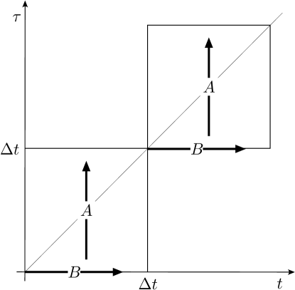
Figure 1. A schematic view of Godunov splitting.

Our Godunov splitting method is given by the following definition.

Definition 3.1 (Godunov splitting).

With $\Delta t>0$ given, define the domain

$$\Omega_{\Delta t}=\bigcup_{n=0}^{\lfloor T/\Delta t\rfloor-1}[t_{n},t_{n+1}]\times[t_{n},t_{n+1}].$$

The time-continuus Godunov splitting solution $\vartheta:\Omega_{\Delta t}\to\mathbb{R}$ is defined as the solution to

$$\begin{split}&\vartheta(0,0)=\theta_{0},\\ &\begin{cases}\vartheta_{t}(t,t_{n})=B(\vartheta(t,t_{n})),&t\in(t_{n},t_{n+1}],\\ \vartheta|_{t=t_{n}}=\theta^{n};\end{cases}\\ &\begin{cases}\vartheta_{\tau}(t,\tau)=A(\vartheta(t,\tau)),&(t,\tau)\in[t_{n},t_{n+1}]\times(t_{n},t_{n+1}],\\ \vartheta|_{\tau=t_{n}}=\vartheta(t,t_{n}),&t\in[t_{n},t_{n+1}],\end{cases}\end{split}$$ (3.1)

cf. Figure 1.

Observe that

$$\vartheta(t_{n},t_{n})=\theta^{n},\quad n=0,\ldots,\lfloor T/\Delta t\rfloor.$$

Thus, $\vartheta(t,t)$ is an extension of $\{\theta^{n}\}_{n}$ to all of $[0,T]$.

To measure the error, we will use the function

$$e(t)=\vartheta(t,t)-\theta(t),$$

where $\theta$ is the (smooth) solution of (1.1).

It is not trivial trivial to obtain the existence of a splitting solution $\vartheta$ in the sense of Definition 3.1. Since the best available existence result we have for the hyperbolic step is local-in-time, it is unclear if we can iterate the steps up to any given large time $T$. In fact, well-posedness of the method is one of our main results.

The following theorem is our main result in this section.

Theorem 3.2.

Suppose $\theta_{0}\in H^{k}$ with $6\leq k\in\mathbb{N}$, and that $\alpha$, $\beta$ $\in[1,2]$. Then, for $\Delta t$ sufficiently small, we have the following:

1. The Godunov splitting approximation $\vartheta(t,\tau)$ is well-defined. Moreover, $\vartheta(t,\tau)$ belongs to $C([0,T]^{2};H^{k})$.

2. The error $e(t):=\|\vartheta(t,t)-\theta(t)\|_{H^{k-2}}$ satisfies

   $$\|e(t)\|_{H^{k-2}}\leq tC\Delta t\|\theta_{0}\|_{H^{k}}^{2}.$$

Theorem 3.2 will be an outcome of the results proved in the subsections below (Subsection 3.3 will bring the pieces together).

3.1. Evolution equations for the error

To prove Theorem 3.2, we will analyze a set of evolution equations satisfied by the error $e$, see [10], which we now derive.

We shall need the following Taylor expansion satisfied by an operator $E$:

$$E(f+g) =E(f)+dE(f)[g]+\int_{0}^{1}(1-\gamma)d^{2}E(f+\gamma g)[g]^{2}~{}d\gamma.$$

Using the definition of $\vartheta$ and the above Taylor formula, we deduce

$$\begin{split}e_{t}-dC(\theta)[e]&=\vartheta_{t}+\vartheta_{\tau}-\theta_{t}-dA(\theta)[e]-dB(\theta)[e]\\ &=\vartheta_{t}+A(\vartheta)-(A+B)(\theta)-dA(\theta)[e]-dB(\theta)[e]\\ &=\vartheta_{t}-B(\vartheta)+(A(\vartheta)-A(\theta)-dA(\theta)[e])\\ &\qquad\qquad+(B(\vartheta)-B(\theta)-dB(\theta)[e])\\ &=F(t,t)+\int_{0}^{1}(1-\gamma)d^{2}C(\theta+\gamma e)[e]^{2}~{}d\gamma,\end{split}$$ (3.2)

where we have introduced the “forcing” term

$$F(t,\tau)=\vartheta_{t}(t,\tau)-B(\vartheta(t,\tau)).$$

By direct calculation,

$$\begin{split}F_{\tau}-dA(\vartheta)[F]&=v_{t\tau}-B(\vartheta)_{\tau}-dA(\vartheta)[\vartheta_{t}-B(\vartheta)]\\ &=A(\vartheta)_{t}-dB(\vartheta)[\vartheta_{\tau}]-dA(\vartheta)[\vartheta_{t}]+dA(\vartheta)[B(\vartheta)]\\ &=dA(\vartheta)[\vartheta_{t}]-dB(\vartheta)[A(\vartheta)]-dA(\vartheta)[\vartheta_{t}]+dA(\vartheta)[B(\vartheta)]\\ &=[A,B](\vartheta),\end{split}$$ (3.3)

where we have defined the commutator

$$\begin{split}[A,B](f)=dA(f)[B(f)]-dB(f)[A(f)].\end{split}$$

For the fluid equation (1.1), we have that

$$\begin{split}A(f)&=-\Lambda^{\alpha}f,\\ dA(f)[g]&=-\Lambda^{\alpha}g,\\ d^{2}A(f)[g,h]&=0,\end{split}$$

and

$$\begin{split}B(f)&=-\nabla f\cdot\operatorname{curl}\Lambda^{-\beta}f,\\ dB(f)[g]&=-\nabla f\cdot\operatorname{curl}\Lambda^{-\beta}g-\nabla g\cdot\operatorname{curl}\Lambda^{-\beta}f,\\ d^{2}B(f)[g,h]&=-\nabla h\cdot\operatorname{curl}\Lambda^{-\beta}g-\nabla g\cdot\operatorname{curl}\Lambda^{-\beta}h.\end{split}$$

The Leibniz formula (Lemma 2.3) yields

$$\begin{split}[A,B](f)&=\Lambda^{\alpha}\left(\nabla f\cdot\operatorname{curl}\Lambda^{-\beta}f\right)\\ &\qquad-\nabla f\cdot\operatorname{curl}\Lambda^{-\beta}\Lambda^{\alpha}f-\left(\nabla\Lambda^{\alpha}f\right)\cdot\operatorname{curl}\Lambda^{-\beta}f\\ &=G^{\alpha}(\nabla f,\operatorname{curl}\Lambda^{-\beta}f).\end{split}$$

Hence, for the fluid equation (1.1), equations (3.2)–(3.3) read:

$$F =\vartheta_{t}+\nabla\vartheta\cdot\operatorname{curl}\Lambda^{-\beta}\vartheta,$$

$$F_{\tau}+\Lambda^{\alpha}F =G^{\alpha}(\nabla\vartheta,\operatorname{curl}\Lambda^{-\beta}\vartheta),$$ (3.4)

$$e_{t}+\Lambda^{\alpha}e =F-\nabla e\cdot\operatorname{curl}\Lambda^{-\beta}\theta-\nabla\theta\cdot\operatorname{curl}\Lambda^{-\beta}e-\nabla e\cdot\operatorname{curl}\Lambda^{-\beta}e.$$ (3.5)

The equations (3.4) and (3.5) constitute our main tool for proving Theorem 3.2.

3.2. Estimates on the error

Lemma 3.5 below provides an estimate on the error $e$ that will be a key ingredient in the proof of Theorem 3.2. The estimate depends on two auxiliary results (Lemmas 3.3 and 3.4) that we first prove.

The first auxiliary results gives perhaps the most fundamental property of our splitting solution. It states that if the splitting solution is in $H^{k}$, $k\geq 6$, then it is actually in $H^{k+2}$.

For notational convenience, let $\Omega_{\Delta t}^{t,\tau}$ denote the set of all times prior to $(t,\tau)$:

$$\Omega_{\Delta t}^{t,\tau}=\{(s,\sigma)\in\Omega_{\Delta t}\mid 0\leq s\leq t,~{}0\leq\sigma\leq\tau\}=\Omega_{\Delta t}\cap\big{(}[0,t]\times[0,\tau]\big{)}.$$

Lemma 3.3.

Assume that $\alpha$, $\beta$ $\in[1,2]$, $6\leq k\in\mathbb{N}$, and let $\vartheta$ be the Godunov approximation to (1.1) in the sense of Definition 3.1 and (3.1).

If for some $(s,\sigma)\in\Omega_{\Delta}$,

$$\|\vartheta(s,\sigma)\|_{H^{k-2}}\leq\gamma,\quad(s,\sigma)\in\Omega_{\Delta t}^{t,\tau},$$ (3.6)

then

$$\|\vartheta(s,\sigma)\|_{H^{k}}\leq e^{C\gamma s}\|\theta_{0}\|_{H^{k}},\quad(s,\sigma)\in\Omega_{\Delta t}^{t,\tau}.$$

Proof.

By direct calculation we see that

$$\begin{split}\partial_{\tau}\frac{1}{2}\|\vartheta(t,\tau)\|_{H^{k}}^{2}&=\sum_{\ell=0}^{k}\int_{\mathbb{R}^{2}}\nabla^{\ell}\vartheta_{\tau}:\nabla^{\ell}\vartheta~{}dx\\ &=-\sum_{\ell=0}^{k}\int_{\mathbb{R}^{2}}\left|\nabla^{\ell}\Lambda^{\alpha/2}\vartheta\right|^{2}~{}dx=-\|\vartheta\|_{H^{k+\alpha/2}}^{2}.\end{split}$$

Hence, for $(t,\tau)\in[t_{n},t_{n+1}]\times(t_{n},t_{n+1}]$, $n=0,\ldots,\lfloor T/\Delta t\rfloor-1$,

$$\|\vartheta(t,\tau)\|_{H^{k}}^{2}\leq\|\vartheta(t,t_{n})\|_{H^{k}}^{2}.$$

We now calculate a bound on the $H^{k}$ norm of $\vartheta(t,t_{n})$. By definition,

$$\begin{split}\partial_{t}\frac{1}{2}\|\vartheta(t,t_{n})\|_{H^{k}}^{2}&=\sum_{\ell=0}^{k}\int_{\mathbb{R}^{2}}\nabla^{\ell}\vartheta_{t}:\nabla^{\ell}\vartheta~{}dx\\ &=-\sum_{\ell=0}^{k}\int_{\mathbb{R}^{2}}\nabla^{\ell}\left(\nabla\vartheta\cdot\operatorname{curl}\Lambda^{-\beta}\vartheta\right):\nabla^{\ell}\vartheta~{}dx.\end{split}$$ (3.7)

Applying Lemma 2.6 to this identity, we see that

$$\partial_{t}\frac{1}{2}\|\vartheta(t,t_{n})\|_{H^{k}}^{2}\leq C\|\vartheta(t,t_{n})\|_{H^{k-2}}\|\vartheta(t,t_{n})\|_{H^{k}}^{2}.$$ (3.8)

Clearly, this allows us to conclude that

$$\partial_{t}\|\vartheta(t,t_{n})\|_{H^{k}}\leq C\gamma\|\vartheta(t,t_{n})\|_{H^{k}},$$

and integration in time gives

$$\|\vartheta(t,t_{n})\|_{H^{k}}\leq e^{C\gamma(t-t_{n})}\|\vartheta(t_{n},t_{n})\|_{H^{k}}.$$

Consequently,

$$\|\vartheta(t,t_{n})\|_{H^{k}}\leq e^{C\gamma t}\|\theta_{0}\|_{H^{k}},$$

which completes the proof. ∎

The following lemma is our second auxiliary result.

Lemma 3.4.

Let $k$, $t$, and $\tau$ be as in the previous lemma. Then,

$$\|F(s,\sigma)\|_{H^{k-2}}\leq\Delta t\,C_{1}e^{C_{2}\gamma s}\|\theta_{0}\|^{2}_{H^{k}},\quad(s,\sigma)\in\Omega^{t,\tau}_{\Delta t}.$$

Proof.

Applying $\nabla^{s}$ to (3.4), multiplying componentwise with $\nabla^{s}F$, summing over $s=0,\ldots,k-2$, and integrating over the domain gives

$$\begin{split}&\partial_{\tau}\frac{1}{2}\|F\|_{H^{k-2}}^{2}+\|F\|_{H^{k-2+\alpha/2}}^{2}\\ &\qquad\qquad=\sum_{s=0}^{k-2}\int_{\mathbb{R}^{2}}\nabla^{s}F:\nabla^{s}G^{\alpha}(\nabla\vartheta,\operatorname{curl}\Lambda^{-\beta}\vartheta)~{}dx\\ &\qquad\qquad\leq C\|F\|_{H^{k-2}}\|G^{\alpha}(\nabla\vartheta,\operatorname{curl}\Lambda^{-\beta}\vartheta)\|_{H^{k-2}}.\end{split}$$ (3.9)

An application of Corollary 2.5 to (3.9) gives (here we do not make use of the regularizing effect of $\Lambda^{-\beta}$)

$$\begin{split}\partial_{\tau}\frac{1}{2}\|F\|_{H^{k-2}}^{2}\leq C\|F\|_{H^{k-2}}\|\nabla\vartheta\|_{H^{k-1}}\|\operatorname{curl}\Lambda^{-\beta}\vartheta\|_{H^{k-1}}\leq C\|F\|_{H^{k-2}}\|\vartheta\|_{H^{k}}^{2}.\end{split}$$

In view of Lemma 3.3, this means that

$$\partial_{\tau}\|F\|_{H^{k-2}}\leq C_{1}e^{C_{2}\gamma t}\|\theta_{0}\|_{H^{k}}^{2}.$$

Since $F(t,t_{n})=0$ integration in time gives

$$\|F\|_{H^{k-2}}\leq\Delta t\,C_{1}e^{C_{2}\gamma t}\|\theta_{0}\|_{H^{k}}^{2},$$

which concludes the proof. ∎

The next lemma will be the key ingredient in the proof of Theorem 3.2.

Lemma 3.5.

Let $k$, $t$, and $\tau$ be as in Lemma 3.3. Then,

$$\|e(s)\|_{H^{k-2}}\leq s\Delta t\,C_{1}e^{c\gamma t}\|\theta_{0}\|_{H^{k}}^{2},\quad 0<s\leq t.$$

Proof.

Applying $\nabla^{s}$ to (3.5), multiplying componentwise with $\nabla^{s}e$, summing over $s=0,\ldots,k-2$, and integrating gives

$$\begin{split}&\frac{1}{2}\partial_{t}\|e\|_{H^{s}}^{2}+\|e\|_{H^{s+\alpha/2}}^{2}\\ &\qquad=\sum_{s=0}^{k-2}\int_{\mathbb{R}^{2}}\Big{[}\nabla^{s}F\,:\nabla^{s}e+\nabla^{s}\left(\nabla e\cdot\operatorname{curl}\Lambda^{-\beta}e\right):\nabla^{s}e\\ &\qquad\qquad-\nabla^{s}\left(\nabla\theta\cdot\operatorname{curl}\Lambda^{-\beta}e+\nabla e\cdot\operatorname{curl}\Lambda^{-\beta}\theta\right):\nabla^{s}e\Big{]}dx\\ &\qquad\leq\|e\|_{H^{k-2}}\|F\|_{H^{k-2}}+\sum_{s=0}^{k-2}\int_{\mathbb{R}^{2}}|\,\nabla^{s}\left(\nabla e\cdot\operatorname{curl}\Lambda^{-\beta}e\right):\nabla^{s}e\\ &\qquad\qquad-\sum_{s=0}^{k-2}\nabla^{s}\left(\nabla\theta\cdot\operatorname{curl}\Lambda^{-\beta}e+\nabla e\cdot\operatorname{curl}\Lambda^{-\beta}\theta\right):\nabla^{s}e\,|~{}dx.\end{split}$$ (3.10)

An application of Lemma 2.6 provides the estimate

$$\begin{split}&\sum_{s=0}^{k-2}\int_{\mathbb{R}^{2}}\nabla^{s}\left(\nabla e\cdot\operatorname{curl}\Lambda^{-\beta}e\right):\nabla^{s}e~{}dx\leq C\|e\|_{H^{k-2}}^{3}\\ &\qquad\leq C\|e\|_{H^{k-2}}^{2}\left(\|\vartheta\|_{H^{k-2}}+\|\theta\|_{H^{k-2}}\right)\leq C\|e\|_{H^{k-2}}^{2}\left(\gamma+\|\theta_{0}\|_{H^{k-2}}\right),\end{split}$$ (3.11)

where we have also used that $\|\vartheta\|_{H^{k-2}}\leq\gamma$.

By virtue of Lemma 2.7, we also have the estimate

$$\begin{split}&\sum_{s=0}^{k-2}\int_{\mathbb{R}^{2}}\nabla^{s}\left(\nabla\theta\cdot\operatorname{curl}\Lambda^{-\beta}e+\nabla e\cdot\operatorname{curl}\Lambda^{-\beta}\theta\right):\nabla^{s}e~{}dx\\ &\qquad\leq C\left(\|\theta\|_{H^{k-1}}\|e\|_{H^{k-2}}^{2}+\|\theta\|_{H^{k-2}}\|e\|_{H^{k-2}}^{2}\right).\end{split}$$ (3.12)

Combining (3.12), (3.11), and applying the result together with Lemma 3.4 to (3.10) enable us to conclude that

$$\partial_{t}\|e\|_{H^{k-2}}\leq\Delta t\,C_{1}e^{C_{2}\gamma t}\|\theta_{0}\|_{H^{k}}^{2}+C(\gamma+\|\theta^{0}\|_{H^{k}})\|e\|_{H^{k-2}}.$$

An application of the Gronwall inequality (recalling that $e(0)=0$) yields the result. ∎

3.3. Proof of Theorem 3.2

We will make use of the following bootstrap lemma (cf. [21, Proposition 1.21]):

Lemma 3.6.

For each $(t,\tau)\in\Omega_{\Delta t}$, suppose that we have two statements, a “hypothesis” ${\bm{H}}(t,\tau)$ and a “conclusion” ${\bm{C}}(t,\tau)$. Suppose that we can verify the following assertions:

1. If ${\bm{H}}(t,\tau)$ is true for some $(t,\tau)\in\Omega_{\Delta t}$, then ${\bm{C}}(t,\tau)$ is also true.

2. If ${\bm{C}}(t,\tau)$ is true for some $(t,\tau)\in\Omega_{\Delta t}$, then ${\bm{H}}(t^{\prime},\tau^{\prime})$ is also true for all $(t^{\prime},\tau^{\prime})$ in a neighborhood of $(t,\tau)$.

3. If $(t_{1},\tau_{1})$, $(t_{2},\tau_{2})$, $\ldots$ is a sequence in $\Omega_{\Delta t}$ converging to $(t,\tau)\in\Omega_{\Delta t}$, and ${\bm{C}}(t_{n},\tau_{n})$ is true for all $n$, then ${\bm{C}}(t,\tau)$ is true.

4. ${\bm{H}}(t,\tau)$ is true for at least one $(t,\tau)\in\Omega_{\Delta t}$.

Then ${\bm{C}}(t,\tau)$ is true for all $(t,\tau)\in\Omega_{\Delta t}$.

Let ${\bm{H}}(t,\tau)$ denote the statement

$$\|\vartheta(s,\sigma)\|_{H^{k-2}}\leq\gamma,\quad(s,\sigma)\in\Omega^{t,\tau}_{\Delta t},$$

and ${\bm{C}}(t,\tau)$ the statement

$$\|\vartheta(s,\sigma)\|_{H^{k-2}}\leq\frac{\gamma}{2},\quad(s,\sigma)\in\Omega^{t,\tau}_{\Delta t},$$

where $\gamma$ is some value which will specified below. Let us for a moment assume that assertions (1)–(4) of Lemma 3.6 are true for ${\bm{H}}$ and ${\bm{C}}$. In this case Lemma 3.6 tells us that ${\bm{C}}(t,\tau)$ holds for all $(t,\tau)\in\Omega_{\Delta t}$. Hence, the $H^{k-2}$ norm of the splitting solution never blows up and thus the existence part of Theorem 3.2 follows readily (a local-in-time solution can be extended to all of $(0,T)$).

Let us now verify assertions (1)–(4) of Lemma 3.6 for our choice of ${\bm{H}}(t,\tau)$ and ${\bm{C}}(t,\tau)$. First, we observe that assertions (2) and (3) clearly hold. For assertion (4) to be true, we assume that $\gamma$ satisfies

$$\|\vartheta(0,0)\|_{H^{k-2}}=\|\theta_{0}\|_{H^{k-2}}\leq\gamma.$$ (3.13)

Then it remains to verify assertion (1). For this purpose, let us assume that ${\bm{H}}(t,\tau)$ is true for some $(t,\tau)\in\Omega_{\Delta t}$. Lemma 3.5 can then be applied to obtain the bound

$$\|e(s)\|_{H^{k-2}}\leq s(\Delta t)Ce^{c\gamma t}\|\theta_{0}\|_{H^{k}}^{2},\quad s\in[0,t].$$ (3.14)

We need to compare $\vartheta(s,\sigma)$ with the corresponding value on the diagonal, viz.  $\vartheta(s,s)$. Two cases need to be considered:
(i) If $\sigma>s$, we observe that

$$\partial_{\sigma}\frac{1}{2}\|\vartheta(s,\sigma)\|_{H^{k-2}}^{2}=\sum_{s=0}^{k-2}\int_{\mathbb{R}^{2}}\nabla^{s}\vartheta_{\sigma}:\nabla^{s}\vartheta~{}dx\\ =-\sum_{s=0}^{k-2}\int_{\mathbb{R}^{2}}|\nabla^{s}\Lambda^{\alpha/2}\vartheta|~{}dx\leq 0,$$

(using that $\alpha\leq 2$ to make sure the expression is finite) which implies that
$\|\vartheta(s,\sigma)\|_{H^{k-2}}\leq\|\vartheta(s,s)\|_{H^{k-2}}$.
(ii) If $\sigma<s$ we first see that

$$\begin{split}\left|\partial_{\sigma}\frac{1}{2}\|\vartheta(s,\sigma)\|_{H^{k-2}}^{2}\right|&=\left|\sum_{s=0}^{k-2}\int_{\mathbb{R}^{2}}\nabla^{s}\vartheta_{\sigma}:\nabla^{s}\vartheta~{}dx\right|\\ &=\left|\sum_{s=0}^{k-2}\int_{\mathbb{R}^{2}}\nabla^{s}\Lambda^{\alpha}\vartheta:\nabla^{s}\vartheta~{}dx\right|\leq\|\vartheta(s,\sigma)\|_{H^{k-2}}\|\vartheta(s,\sigma)\|_{H^{k}},\end{split}$$

(using $\alpha\leq 2$) which implies that

$$\left|\partial_{\sigma}\|\vartheta(s,\sigma)\|_{H^{k-2}}\right|\leq\|\vartheta(s,\sigma)\|_{H^{k}}.$$

Using this inequality and applying Lemma 3.3 we find

$$\begin{split}\|\vartheta(s,\sigma)\|_{H^{k-2}}&\leq\|\vartheta(s,s)\|_{H^{k-2}}+\int_{\sigma}^{s}|\partial_{\sigma}\|\vartheta(s,\tilde{\sigma})\||~{}d\tilde{\sigma}\\ &\leq\|\vartheta(s,s)\|_{H^{k-2}}+\Delta t\sup_{\sigma^{\prime}\in[\sigma,s]}\|\vartheta(s,\sigma^{\prime})\|_{H^{k}}\\ &\leq\|\vartheta(s,s)\|_{H^{k-2}}+\Delta t\,e^{C\gamma s}\|\theta_{0}\|_{H^{k}}.\end{split}$$

Thus in both cases we conclude that

$$\|\vartheta(s,\sigma)\|_{H^{k-2}}\leq\|\vartheta(s,s)\|_{H^{k-2}}+\Delta t\,e^{C\gamma s}\|\theta_{0}\|_{H^{k}},\quad|s-\sigma|\leq\Delta t.$$

By applying the previous inequality, adding and subtracting $\theta$, and involving (3.14), we estimate

$$\begin{split}\|\vartheta(s,\sigma)\|_{H^{k-2}}&\leq\|e(s)\|_{H^{k-2}}+\|\theta(s)\|_{H^{k-2}}+\Delta t\,e^{C\gamma s}\|\theta_{0}\|_{H^{k}}\\ &\leq C\Delta t\,e^{C\gamma T}(s\|\theta_{0}\|^{2}_{H^{k}}+\|\theta_{0}\|_{H^{k}}\big{)}+C\|\theta_{0}\|_{H^{k}}\\ &\leq\Delta t\,C_{1}(\gamma)+C_{2}.\end{split}$$ (3.15)

Now, we fix $\gamma$ and $\Delta t$ according to

$$\gamma=4C_{2},\qquad\Delta t\leq\frac{C_{2}}{C_{1}(\gamma)},$$

and note that this is not conflict with (3.13).

Then, (3.15) gives

$$\begin{split}\|\vartheta(s,\sigma)\|_{H^{k-2}}\leq 2C_{2}=\frac{\gamma}{2},\quad(s,\sigma)\in\Omega^{t,\tau}_{\Delta t},\end{split}$$

which verifies (1) in Lemma 3.6.

At this point we have verified assertions (1)–(4) of Lemma 3.6 for our choice of ${\bm{H}}(t,\tau)$ and ${\bm{C}}(t,\tau)$. Consequently, Lemma 3.6 tells us that ${\bm{C}}(t,\tau)$ is true for all times $(t,\tau)\in\Omega_{\Delta t}$. In other words,

$$\|\vartheta(t,\tau)\|_{H^{k-2}}\leq\frac{\gamma}{2},\quad(t,\tau)\in\Omega_{\Delta t},$$ (3.16)

which concludes the existence part of Theorem 3.2.

Equipped with (3.16), we can apply Lemma 3.5 to obtain the error estimate

$$\|e(t)\|_{H^{k-2}}\leq t\Delta t\,Ce^{Ct}\|\theta_{0}\|^{2}_{H^{k}},\quad t\in[0,T],$$

which is the second part of Theorem 3.2.∎

4. Strang splitting

In this section we prove the expected second-order convergence rate of Strang splitting applied to (1.1). We also prove that the method produces regular solutions up to any given finite final time $T>0$. The results are valid under a condition on the size of each time step $\Delta t$.

We will continue to use the notation and definitions introduced in the previous section, unless explicitly stating otherwise. The Strang method we consider in this section reads as follows: For $\Delta t>0$ given, construct a sequence $\{\theta^{n}\}_{n=0}^{\lfloor T/\Delta t\rfloor}$ of approximate solutions to (1.1) by the following procedure: Let $\theta^{0}=\theta_{0}$ and determine sequentially

$$\begin{split}\theta^{n+1}&=\Phi_{B}\left(\frac{\Delta t}{2},\Phi_{A}(\Delta t,\Phi_{B}(\frac{\Delta t}{2},\theta^{n}))\right)\\ &=\left[\Phi_{B}(\frac{\Delta t}{2})\circ\Phi_{A}(\Delta t)\circ\Phi_{B}(\frac{\Delta t}{2})\right](\theta^{n}).\end{split}$$

As with the Godunov splitting, the convergence analysis will require a time-continuous interpolation of the Strang approximations $\{\theta^{n}\}_{n}$. In contrast to the Godunov case, we will now introduce three time variables instead of two. This approach is different from the one taken in [10], and indeed appears more natural. In [10] the authors stick to two time variables and interpret Strang splitting in terms of two “$\Delta t/2$” Godunov splittings, and in alternating order.

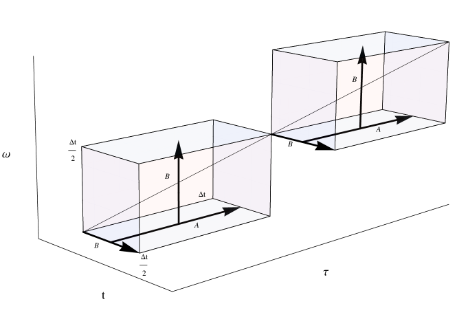
Figure 2. A schematic view of Strang splitting.

Definition 4.1 (Strang splitting).

With $\Delta t>0$ given, define the domain

$$\Omega_{\Delta t}=\bigcup_{n=0}^{\lfloor T/\Delta t\rfloor-1}\left[\frac{t_{n}}{2},\frac{t_{n+1}}{2}\right]\times\left[t_{n},t_{n+1}\right]\times\left[\frac{t_{n}}{2},\frac{t_{n+1}}{2}\right].$$

The time-continuous Strang splitting solution $\vartheta:\Omega_{\Delta t}\to\mathbb{R}$ is defined as

$$\begin{split}&\vartheta(0,0,0)=\theta_{0},\\ &\begin{cases}\vartheta_{t}\left(t,t_{n},\frac{t_{n}}{2}\right)=B\left(\vartheta\left(t,t_{n},\frac{t_{n}}{2}\right)\right),&t\in\left(\frac{t_{n}}{2},\frac{t_{n+1}}{2}\right],\\ \vartheta|_{t=\frac{t_{n}}{2}}=\theta^{n};\end{cases}\\ &\begin{cases}\vartheta_{\tau}\left(t,\tau,\frac{t_{n}}{2}\right)=A\left(\vartheta\left(t,\tau,\frac{t_{n}}{2}\right)\right),&(t,\tau)\in\left[\frac{t_{n}}{2},\frac{t_{n+1}}{2}\right]\times\left(t_{n},t_{n+1}\right],\\ \vartheta|_{\tau=t_{n}}=\vartheta\left(t,t_{n},\frac{t_{n}}{2}\right),&t\in\left[\frac{t_{n}}{2},\frac{t_{n+1}}{2}\right];\end{cases}\\ &\begin{cases}\vartheta_{\omega}(t,\tau,\omega)=B\left(\vartheta\left(t,\tau,\omega\right)\right),&(t,\tau,\omega)\in\left[\frac{t_{n}}{2},\frac{t_{n+1}}{2}\right]\times[t_{n},t_{n+1}]\times\left(\frac{t_{n}}{2},\frac{t_{n+1}}{2}\right),\\ \vartheta|_{\omega=\frac{t_{n}}{2}}=\vartheta\left(t,\tau,\frac{t_{n}}{2}\right),&(t,\tau)\in\left[\frac{t_{n}}{2},\frac{t_{n+1}}{2}\right],\end{cases}\end{split}$$ (4.1)

cf. Figure 2.

In each box $\left[\frac{t_{n}}{2},\frac{t_{n+1}}{2}\right]\times\left[t_{n},t_{n+1}\right]\times\left[\frac{t_{n}}{2},\frac{t_{n+1}}{2}\right]$, it is of particular interest to consider the function $\vartheta$ restricted to the diagonal, i.e., the function $\vartheta\left(\frac{t}{2},t,\frac{t}{2}\right)$ for $t\in[t_{n},t_{n+1}]$. Observe that at each point on the diagonal, $\vartheta$ is a Strang splitting solution with a specific time step. Specifically, $\vartheta\left(\frac{t}{2},t,\frac{t}{2}\right)$ is a Strang splitting solution with time step $t-t_{n}$. Consequently,

$$\vartheta\left(\frac{t_{n}}{2},t_{n},\frac{t_{n}}{2}\right)=\theta^{n},\quad n=0,\ldots,\lfloor T/\Delta t\rfloor,$$

and hence that $\vartheta\left(\frac{t}{2},t,\frac{t}{2}\right)$ can be seen as an extension of $\{\theta^{n}\}_{n}$ to all of $[0,T]$.

To measure the error between the splitting approximation and the exact solution, we will use the function

$$e(t)=\vartheta\left(\frac{t}{2},t,\frac{t}{2}\right)-\theta(t),$$

where $\theta$ is the (smooth) solution of (1.1).

We state two main results in this section.

Lemma 4.2 (Well-defined).

Let $\vartheta=\vartheta(t,\tau,\omega)$ be the Strang splitting solution of (1.1) in the sense of Definition 4.1. Suppose $\theta_{0}\in H^{k}$ with $6\leq k\in\mathbb{N}$, $\alpha$, $\beta$ $\in[1,2]$, and that $\Delta t>0$ is sufficiently small. Then

1. the Strang splitting method is well-defined with $\vartheta\in C([0,T]^{2};H^{k})$;

2. the error $e(t)=\vartheta(\frac{t}{2},t,\frac{t}{2})-\theta(t)$ satisfies

   $$\|e(t)\|_{H^{k-2}}\leq C\,t\,\Delta t.$$

   for some constant $C=C\left(\|\theta_{0}\|_{H^{k}}\right)$.

Theorem 4.3 (Convergence).

Under the conditions of the previous lemma,

$$\|e(t)\|_{H^{k-3\alpha}}\leq C(\Delta t)^{2},$$

for some constant $C=C\left(\|\theta_{0}\|_{H^{k}}\right)$.

Lemma 4.2 and Theorem 4.3 will be consequences of the results stated and proved in the ensuing subsections.

4.1. The error evolution equations

To prove Lemma 4.2 we will use the same approach as for the Godunov method. However, since we are now using three time variables instead of two, we must derive a new set of evolution equations governing the error.

By a direct calculation, the error $e$ satisfies the time-evolution

$$\begin{split}e_{t}-dC(\theta)[e]&=\frac{\vartheta_{t}}{2}+\vartheta_{\tau}+\frac{\vartheta_{\omega}}{2}-\theta_{t}-dA(\theta)[e]-dB(\theta)[e]\\ &=\frac{\vartheta_{t}}{2}+\vartheta_{\tau}+\frac{1}{2}B(\vartheta)-(A+B)(\theta)-dA(\theta)[e]-dB(\theta)[e]\\ &=\frac{1}{2}\left(\vartheta_{t}-B(\vartheta)\right)+\vartheta_{\tau}-A(\vartheta)\\ &\qquad+(A(\vartheta)-A(\theta)-dA(\theta)[e])+(B(\vartheta)-B(\theta)-dB(\theta)[e])\\ &=F(t)+\int_{0}^{1}(1-\gamma)d^{2}C(\theta+\gamma e)[e]^{2}~{}d\gamma,\end{split}$$

where $F(t)=F\left(\frac{t}{2},t,\frac{t}{2}\right)$ and

$$F(t,\tau,\omega)=\frac{1}{2}\left(\vartheta_{t}(t,\tau,\omega)-B(\vartheta(t,\tau,\omega))\right)+\vartheta_{\tau}-A(\vartheta(t,\tau,\omega)).$$

Since $\vartheta_{\tau}-A(\vartheta(t,\tau,\omega))=0$ when $\omega=\frac{t_{n}}{2}$, $n=0,\ldots,\lfloor T/\Delta t\rfloor-1$, we can apply the arguments of (3.3) to obtain

$$F_{\tau}-dA(\vartheta)[F]=\frac{1}{2}[A,B](\vartheta),\quad\left(t,\tau,\frac{t_{n}}{2}\right)\in\Omega_{\Delta t},$$

where

$$[A,B](f)=dA(f)[B(f)]-dB(f)[A(f)].$$

We also derive the following equation for the evolution of $F$ in $\omega$:

$$\begin{split}&F_{\omega}-dB(\vartheta)[F]\\ &\qquad=\frac{1}{2}\vartheta_{t\omega}-\frac{1}{2}B(\vartheta)_{\omega}-\frac{1}{2}dB(\vartheta)[\vartheta_{t}-B(\vartheta)]\\ &\qquad\qquad+\vartheta_{\tau\omega}-dA(\vartheta)[\vartheta_{\omega}]-dB(\vartheta)[\vartheta_{\tau}-A(\vartheta)]\\ &\qquad=\frac{1}{2}B(\vartheta)_{t}-\frac{1}{2}dB(\vartheta)[\vartheta_{\omega}]-\frac{1}{2}dB(\vartheta)[\vartheta_{t}]+\frac{1}{2}dB(\vartheta)[B(\vartheta)]\\ &\qquad\qquad+dB(\vartheta)[\vartheta_{\tau}]-dA(\vartheta)[B(\vartheta)]-dB(\vartheta)[\vartheta_{\tau}]+dB(\vartheta)[A(\vartheta)]\\ &\qquad=\frac{1}{2}\left(dB(\vartheta)[\vartheta_{t}]-dB(\vartheta)[B(\vartheta)]-dB(\vartheta)[\vartheta_{t}]+dB(\vartheta)[B(\vartheta)]\right)\\ &\qquad\qquad+dB(\vartheta)[A(\vartheta)]-dA(\vartheta)[B(\vartheta)]\\ &\qquad=dB(\vartheta)[A(\vartheta)]-dA(\vartheta)[B(\vartheta)].\end{split}$$

Thus, recalling the definition of $[\,\cdot\,,\,\cdot\,]$,

$$F_{\omega}-dB(\vartheta)[F]=[B,A](\vartheta).$$

For (1.1) the above evolution equations take the form:

$$F =\frac{1}{2}\left(\vartheta_{t}+\nabla\vartheta\cdot\operatorname{curl}\Lambda^{-\beta}\vartheta\right)+\vartheta_{\tau}+\Lambda^{\alpha}\vartheta,\quad(t,\tau,\omega)\in\Omega_{\Delta t},$$

$$F_{\tau}+\Lambda^{\alpha}F =\frac{1}{2}G^{\alpha}(\nabla\vartheta,\operatorname{curl}\Lambda^{-\beta}\vartheta),\quad\omega=\frac{t_{n}}{2},\,n=0,\ldots,\lfloor T/\Delta t\rfloor,$$ (4.2)

$$F_{\omega} =-\nabla\vartheta\cdot\operatorname{curl}\Lambda^{-\beta}F-\nabla F\cdot\operatorname{curl}\Lambda^{-\beta}\vartheta$$

$$\qquad-G^{\alpha}(\nabla\vartheta,\operatorname{curl}\Lambda^{-\beta}\vartheta),\quad(t,\tau,\omega)\in\Omega_{\Delta t},$$ (4.3)

$$e_{t}+\Lambda^{\alpha}e =F-\nabla e\cdot\operatorname{curl}\Lambda^{-\beta}\theta-\nabla\theta\cdot\operatorname{curl}\Lambda^{-\beta}e$$

$$\qquad-\nabla e\cdot\operatorname{curl}\Lambda^{-\beta}e,\quad(t,\tau,\omega)\in\Omega_{\Delta t}.$$ (4.4)

To prove Lemma 4.2 we will adapt Lemmas 3.3, 3.4, and 3.5 to the Strang splitting approximation.

Let $\Omega_{\Delta t}^{t,\tau,\omega}$ denote the set of times prior to $(t,\tau,\omega)$:

$$\Omega_{\Delta t}^{t,\tau,\omega}=\Omega_{\Delta t}\cap\big{(}\,[0,t]\times[0,\tau]\times[0,\omega]\,\big{)}.$$ (4.5)

We begin by observing that Lemma 3.3 can be easily adapted to yield the following result.

Lemma 4.4.

Let $6\leq k\in\mathbb{N}$, and assume the existence of $(t,\tau,\omega)\in\Omega_{\Delta t}$ such that

$$\|\vartheta(s,\sigma,\zeta)\|_{H^{k-2}}\leq\gamma,\qquad(s,\sigma,\zeta)\in\Omega_{\Delta t}^{t,\tau,\omega}.$$ (4.6)

Then

$$\|\vartheta(s,\sigma,\zeta)\|_{H^{k}}\leq e^{C\gamma(s+\zeta)}\|\theta_{0}\|_{H^{k}},\qquad(s,\sigma,\zeta)\in\Omega_{\Delta t}^{t,\tau,\omega}.$$ (4.7)

Next we prove a Strang version of Lemma 3.4.

Lemma 4.5.

Under the conditions of the previous lemma,

$$\|F(s,\sigma,\zeta)\|_{H^{k-2}}\leq\Delta t\,C_{1}e^{C_{2}\gamma(s+\zeta)},\qquad(s,\sigma,\zeta)\in\Omega_{\Delta t}^{t,\tau,\omega}.$$

Proof.

First, we observe that in the plane given by $\omega=\frac{t_{n}}{2}$,

$$F(s,\sigma,\frac{t_{n}}{2})=\frac{1}{2}\left(\vartheta_{t}-B(\vartheta)\right),\quad n=0,\ldots,\lfloor T/\Delta t\rfloor-1.$$

Note that while $F\neq 0$ on the line $(s,t_{n},\frac{t_{n}}{2})$, there holds $\frac{1}{2}\left(\vartheta_{t}-B(\vartheta)\right)=0$ on $(s,t_{n},\frac{t_{n}}{2})$. Hence, we can repeat the arguments of Lemma 3.4 to conclude that

$$\begin{split}\|F(s,\sigma,\frac{t_{n}}{2})\|_{H^{k-2}}&=\|\frac{1}{2}\left(\vartheta_{t}(s,\sigma,\frac{t_{n}}{2})-B(\vartheta(s,\sigma,\frac{t_{n}}{2}))\right)\|_{H^{k-2}}\\ &\leq\Delta t\,C_{1}e^{C_{2}\gamma s},\quad(s,\sigma,\frac{t_{n}}{2})\in\Omega_{\Delta t}^{t,\tau,\omega}.\end{split}$$ (4.8)

We fix $n$ such that $(t,\tau,\omega)\in[\frac{t_{n}}{2},\frac{t_{n+1}}{2}]\times[t_{n},t_{n+1}]\times[\frac{t_{n}}{2},\frac{t_{n+1}}{2}]$. Now, to estimate $\|F\|_{H^{k-2}}$ at an arbitrary point $(s,\sigma,\zeta)\in\Omega_{\Delta t}^{t,\tau,\omega}$, we will first integrate in the $\omega$ direction to the plane given by $\omega=\frac{t_{n}}{2}$ and then apply the estimate (4.8). To perform this integration, we apply $\nabla^{s}$ to (4.3), multiply the result with $\nabla^{s}F$, sum over $s=0,\ldots,k-2$, and integrate by parts, to obtain

$$\begin{split}\partial_{\omega}\frac{1}{2}\|F\|_{H^{k-2}}^{2}&=-\sum_{s=0}^{k-2}\int_{\mathbb{R}^{2}}\nabla^{s}F:\nabla^{s}G^{\alpha}(\nabla\vartheta,\operatorname{curl}\Lambda^{-\beta}\vartheta)~{}dx\\ &\qquad-\sum_{s=0}^{k-2}\int_{\mathbb{R}^{2}}\nabla^{s}\left(\nabla\vartheta\cdot\operatorname{curl}\Lambda^{-\beta}F\right):\nabla^{s}F~{}dx\\ &\qquad-\sum_{s=0}^{k-2}\int_{\mathbb{R}^{2}}\nabla^{s}\left(\nabla F\cdot\operatorname{curl}\Lambda^{-\beta}\vartheta\right):\nabla^{s}F~{}dx\\ &:=I_{1}+I_{2}+I_{3},\end{split}$$ (4.9)

and the goal is to bound the terms $I_{1}$, $I_{2}$, and $I_{3}$.

By first estimating as in (3.9), then using Corollary 2.5, and finally applying Lemma 4.4, we obtain

$$|I_{1}| \leq\|F\|_{H^{k-2}}\|G^{\alpha}(\nabla\vartheta,\operatorname{curl}\Lambda^{-\beta}\vartheta)\|_{H^{k-2}}$$

$$\leq C\|F\|_{H^{k-2}}\|\nabla\vartheta\|_{H^{k-1}}\|\nabla\operatorname{curl}\Lambda^{-\beta}\vartheta\|_{H^{k-1}}$$

$$\leq C_{1}\|F\|_{H^{k-2}}e^{C_{2}\gamma(s+\zeta)}\|\theta_{0}\|_{H^{k}}^{2}.$$

To bound the two other terms $I_{2}$ and $I_{3}$, we first apply Lemma 2.7 to find

$$\begin{split}|I_{2}+I_{3}|\leq C\|F\|_{H^{k-2}}^{2}\|\vartheta\|_{H^{k-1}}.\end{split}$$

An application of Lemma 4.4 then yields

$$\begin{split}|I_{2}+I_{3}|\leq C\|F\|_{H^{k-2}}^{2}e^{C_{2}\gamma(s+\zeta)}\|\theta_{0}\|_{H^{k}}.\end{split}$$

Inserting these bounds back into (4.9),

$$\partial_{\omega}\|F\|_{H^{k-2}}\leq C_{1}e^{C_{2}\gamma(s+\zeta)}+C_{3}\|F\|_{H^{k-2}}.$$

Applying the Gronwall lemma we obtain

$$\|F(s,\sigma,\zeta)\|_{H^{k-2}}\leq e^{C_{3}\gamma\Delta t}\left(\left\|F\left(s,\sigma,\frac{t_{n}}{2}\right)\right\|_{H^{k-2}}+\Delta t\,C_{1}e^{C_{2}\gamma(s+\zeta)}\right).$$

Finally, we apply (4.8) to conclude

$$\|F(s,\sigma,\zeta)\|_{H^{k-2}}\leq\Delta t\,C_{1}e^{C_{2}\gamma(s+\zeta)},$$

which completes the proof. ∎

Lemma 4.6.

Under the conditions of Lemma 4.4,

$$\|e(s)\|_{H^{k-2}}\leq s\Delta t\,C(\gamma),\quad s\in[0,t],$$

where $C(\gamma)$ is a constant depending only on $\gamma$, $T$, and $\|\theta_{0}\|_{H^{k}}$.

Proof.

Since (4.4) is identical to (3.5), we can repeat the proof of Lemma 3.5 step by step (using Lemmas 4.4 and 4.5 instead of Lemmas 3.3 and 3.4) to conclude. ∎

4.2. Proof of Lemma 4.2

Recall that $\Omega_{\Delta t}^{t,\tau,\omega}$ denotes the set of all times prior to $(t,\tau,\omega)$, cf. (4.5). To prove the existence part of Lemma 4.2 we will utilize the same strategy as with did for the Godunov method in the previous section. That is, to apply the bootstrap lemma (Lemma 3.6) with ${\bm{H}}(t,\tau,\omega)$ as the statement

$$\|\vartheta(s,\sigma,\zeta)\|_{H^{k-2}}\leq\gamma,\quad(s,\sigma,\zeta)\in\Omega^{t,\tau,\omega}_{\Delta t},$$ (4.10)

and ${\bm{C}}(t,\tau,\omega)$ the statement

$$\|\vartheta(s,\sigma,\zeta)\|_{H^{k-2}}\leq\frac{\gamma}{2},\quad(s,\sigma,\zeta)\in\Omega^{t,\tau,\omega}_{\Delta t},$$

where $\gamma$ is some value to be specified below. Note that there is no problem with extending Lemma 3.6 so that it allows three time variables instead of two (i.e., hypothesis and statement depending on three variables).

To conclude the existence part of Lemma 4.2 we must verify assertions (1)–(4) in Lemma 3.6. Assertions (2) and (3) clearly hold. Regarding assertion (4), we make the assumption

$$\|\vartheta(0,0,0)\|_{H^{k-2}}=\|\theta_{0}\|_{H^{k-2}}\leq\gamma.$$ (4.11)

It remains to verify assertion (1). For this purpose, let us assume that ${\bm{H}}(t,\tau,\omega)$ is true for some $(t,\tau,\omega)\in\Omega_{\Delta t}$. In order to show assertion (1) we need to prove that ${\bm{C}}(t,\tau,\omega)$ is true. We first note that ${\bm{H}}(t,\tau,\omega)$ being true renders Lemma 4.6 applicable, allowing us to conclude

$$\|e(s)\|_{H^{k-2}}\leq s\Delta t\,C_{1}(\gamma),\quad s\in[0,t].$$ (4.12)

Now, to estimate $\|\vartheta(s,\sigma,\zeta)\|_{H^{k-2}}$ at any time $(s,\sigma,\zeta)\in\Omega_{\Delta t}^{t,\tau,\omega}$ the idea is to consider the time evolution of $\|\vartheta(s,\sigma,\zeta)\|_{H^{k-2}}$ in the $\omega$ and $\tau$ directions. Let $n$ be such that $(t,\tau,\omega)\in[\frac{t_{n}}{2},\frac{t_{n+1}}{2}]\times[t_{n},t_{n+1}]\times[\frac{t_{n}}{2},\frac{t_{n+1}}{2}]$. First we integrate from $(s,\sigma,\zeta)$ to $(s,\sigma,\frac{t_{n}}{2})$. Then, we integrate the result in the plane $\omega=\frac{t_{n}}{2}$ from $(s,\sigma,\frac{t_{n}}{2})$ to $(s,2s,\frac{t_{n}}{2})$. Finally, we integrate in the $\omega$ direction from $(s,2s,\frac{t_{n}}{2})$ to the diagonal $(s,2s,s)$. On the diagonal, we will then utilize (4.12) to conclude the necessary bound.

By definition,

$$\begin{split}\left|\partial_{\omega}\frac{1}{2}\|\vartheta(s,\sigma,\zeta)\|_{H^{k-2}}^{2}\right|&=\left|\sum_{s=0}^{k-2}\int_{\mathbb{R}^{2}}\nabla^{s}\vartheta_{\omega}:\nabla^{s}\vartheta~{}dx\right|\\ &=\left|-\sum_{s=0}^{k-2}\int_{\mathbb{R}^{2}}\nabla^{s}\left(\nabla\vartheta\cdot\operatorname{curl}\Lambda^{-\beta}\vartheta\right):\nabla^{s}\vartheta~{}dx\right|\\ &\leq C\|\vartheta\|_{H^{k-4}}\|\vartheta\|_{H^{k-2}}^{2}\leq\gamma C\|\vartheta(s,\sigma,\zeta)\|_{H^{k-2}}^{2},\end{split}$$ (4.13)

where the estimate follows from Lemma 2.6, and where we have used (4.10). The fundamental theorem of calculus and (4.13) provides us with the estimate

$$\begin{split}\|\vartheta(s,\sigma,\zeta)\|_{H^{k-2}}&\leq\|\vartheta(s,\sigma,\zeta_{2})\|_{H^{k-2}}+C\Delta t\sup_{\zeta^{\prime}\in[\frac{t_{n}}{2},\frac{t_{n+1}}{2}]}\|\vartheta(s,\sigma,\zeta^{\prime})\|_{H^{k-2}}\\ &\leq\|\vartheta(s,\sigma,\zeta_{2})\|_{H^{k-2}}+C\Delta t\,\|\theta_{0}\|_{H^{k-2}},\end{split}$$ (4.14)

for any $\frac{t_{n}}{2}\leq\zeta_{2}\leq\frac{t_{n+1}}{2}$.

Similarly,

$$\begin{split}\left|\partial_{\tau}\frac{1}{2}\left\|\vartheta\left(s,\sigma,\frac{t_{n}}{2}\right)\right\|_{H^{k-2}}^{2}\right|&=\left|\sum_{s=0}^{k-2}\int_{\mathbb{R}^{2}}\nabla^{s}\vartheta_{\tau}:\nabla^{s}\vartheta~{}dx\right|\\ &=\left|-\sum_{s=0}^{k-2}\int_{\mathbb{R}^{2}}\nabla^{s}\Lambda^{\alpha}\vartheta:\nabla^{s}\vartheta~{}dx\right|\\ &\leq\left\|\vartheta\left(s,\sigma,\frac{t_{n}}{2}\right)\right\|_{H^{k-2}}\left\|\vartheta\left(s,\sigma,\frac{t_{n}}{2}\right)\right\|_{H^{k}},\end{split}$$

where we have used that $\alpha\leq 2$. Thus

$$\left|\partial_{\tau}\frac{1}{2}\left\|\vartheta\left(s,\sigma,\frac{t_{n}}{2}\right)\right\|_{H^{k-2}}\right|\leq\left\|\vartheta\left(s,\sigma,\frac{t_{n}}{2}\right)\right\|_{H^{k}}.$$

From the fundamental theorem of calculus, using the previous inequality and Lemma 4.4, we conclude

$$\begin{split}\left\|\vartheta\left(s,\sigma,\frac{t_{n}}{2}\right)\right\|_{H^{k-2}}&\leq\left\|\vartheta\left(s,2s,\frac{t_{n}}{2}\right)\right\|_{H^{k-2}}\\ &\qquad+\Delta t\sup_{\sigma^{\prime}\in[\min\{2s,\sigma\},\max\{2s,\sigma\}]}\left\|\vartheta\left(s,\sigma^{\prime},\frac{t_{n}}{2}\right)\right\|_{H^{k}}\\ &\leq\left\|\vartheta\left(s,2s,\frac{t_{n}}{2}\right)\right\|_{H^{k-2}}+\Delta t\,C\|\theta_{0}\|_{H^{k}}.\end{split}$$ (4.15)

Thus, by combining (4.14) and (4.15),

$$\begin{split}\|\vartheta(s,\sigma,\zeta)\|_{H^{k-2}}&\leq\left\|\vartheta\left(s,\sigma,\frac{t_{n}}{2}\right)\right\|_{H^{k-2}}+C\Delta t\,\|\theta_{0}\|_{H^{k-2}}\\ &\leq\left\|\vartheta\left(s,2s,\frac{t_{n}}{2}\right)\right\|_{H^{k-2}}+\Delta t\,C\,\|\theta_{0}\|_{H^{k}}\\ &\leq\left\|\vartheta\left(s,2s,s\right)\right\|_{H^{k-2}}+\Delta t\,C\,\|\theta_{0}\|_{H^{k}}\\ &\leq\|e(2s)\|_{H^{k-2}}+\|\theta(2s)\|_{H^{k-2}}+\Delta t\,C\,\|\theta_{0}\|_{H^{k}}\\ &\leq C_{1}(\gamma)\Delta t+C_{2},\end{split}$$ (4.16)

where the last inequality is (4.12). Now, we fix $\gamma$ and $\Delta t$ according to

$$\gamma=4C_{2},\qquad\Delta t\leq\frac{C_{2}}{C_{1}(\gamma)},$$

and note that this is not conflict with (4.11). Then, (4.16) gives

$$\begin{split}\|\vartheta(s,\sigma,\zeta)\|_{H^{k-2}}\leq 2C_{2}=\frac{\gamma}{2}.\end{split}$$

Since $(s,\sigma,\zeta)\in\Omega_{\Delta t}^{t,\tau,\omega}$ was arbitrarily chosen, this verifies $(1)$ in Lemma 3.6. We have now verified assertions (1)–(4) of Lemma 3.6 for ${\bm{H}}(t,\tau,\omega)$ and ${\bm{C}}(t,\tau,\omega)$. Consequently, Lemma 3.6 tells us that ${\bm{C}}(t,\tau,\omega)$ is true for all times $(t,\tau,\omega)\in\Omega_{\Delta t}$. In other words,

$$\|\vartheta(t,\tau,\omega)\|_{H^{k-2}}\leq\frac{\gamma}{2},\quad(t,\tau,\omega)\in\Omega_{\Delta t}.$$ (4.17)

Thus, we can conclude the existence part of Lemma 4.2. Since (4.17) holds, we can apply Lemma 3.5 to conclude the error estimate

$$\|e(t)\|_{H^{k-2}}\leq t\Delta t\,C,\quad t\in[0,T],$$

which is the second part of Lemma 4.2.

∎

4.3. Temporal regularity and auxiliary estimates

So far we have focused on the spatial regularity of the splitting solution. To prove Theorem 4.3, we will need regularity in time of $\vartheta$. Since we have introduced three time variables, it is convenient to define a time gradient. We will use the notation

$$\nabla_{t}f=\begin{pmatrix}f_{t}\\ f_{\tau}\\ f_{\omega}\end{pmatrix},\qquad\nabla_{t}^{2}f=\begin{pmatrix}f_{tt}&f_{t\tau}&f_{t\omega}\\ f_{\tau t}&f_{\tau\tau}&f_{\tau\omega}\\ f_{\omega t}&f_{\omega\tau}&f_{\omega\omega}\end{pmatrix},$$

with the obvious extension to higher order (i.e., $\nabla_{t}^{k}f$ for $k$th derivative).

Lemma 4.7.

Let $\alpha\in[1,2]$ and $\vartheta$ be the Strang splitting solution in the sense of Definition 4.1. Then, for any $k$ and $l$ such that $\theta_{0}\in H^{k+\alpha l}$,

$$\|\nabla^{l}_{t}\vartheta\|_{H^{k}}\leq C\left(\|\theta_{0}\|_{H^{k+\alpha l}}\right)\,,\quad(t,\tau,\omega)\in\Omega_{\Delta t}.$$

Proof.

We argue by induction on $l$. For $l=0$, the result is merely an application of Lemma 4.4. Now, let us assume that the bound holds for $l=0,\ldots,q$. To close the induction argument, it remains to show the bound for $l=q+1$.

Let $(t^{\prime},\tau^{\prime},\omega^{\prime})\in\Omega_{\Delta t}$ be arbitrary and fix $n$ such that

$$(t^{\prime},\tau^{\prime},\omega^{\prime})\in\left[\frac{t_{n}}{2},\frac{t_{n+1}}{2}\right]\times\left[t_{n},t_{n+1}\right]\times\left[\frac{t_{n}}{2},\frac{t_{n+1}}{2}\right].$$

An arbitrary component of $\nabla_{t}^{q+1}\vartheta$ can be written in the form

$$\Theta^{q+1}_{i,j,\ell}=\frac{\partial^{q+1}}{\partial t^{i}\partial\tau^{j}\partial\omega^{\ell}}\vartheta,\quad 0\leq i,j,\ell\leq q+1,\quad i+j+\ell=q+1,\quad i,j,\ell\in\mathbb{N}.$$

To estimate the arbitrary component at the point $(t^{\prime},\tau^{\prime},\omega^{\prime})$, we first apply the fundamental theorem of calculus to write

$$\begin{split}\frac{1}{2}\|\Theta_{i,j,\ell}^{q+1}(t^{\prime},\tau^{\prime},\omega^{\prime})\|_{H^{k}}^{2}&=\frac{1}{2}\left\|\Theta_{i,j,\ell}^{q+1}\left(t^{\prime},\tau^{\prime},\frac{t_{n}}{2}\right)\right\|_{H^{k}}^{2}\\ &\quad+\sum_{s=0}^{k}\int_{\frac{t_{n}}{2}}^{\omega^{\prime}}\!\!\int_{\mathbb{R}^{2}}\nabla^{s}\partial_{\omega}\Theta_{i,j,\ell}^{q+1}(t^{\prime},\tau^{\prime},s):\nabla^{s}\Theta_{i,j,\ell}^{q+1}(t^{\prime},\tau^{\prime},s)~{}dxds.\end{split}$$

By applying the definition of $\Theta_{i,j,\ell}^{q+1}$, the definition $\vartheta_{\omega}$ (cf. (4.1)), and the Leibniz rule, we deduce

$$\begin{split}&\int_{\mathbb{R}^{2}}\nabla^{s}\partial_{\omega}\Theta_{i,j,\ell}^{q+1}(t^{\prime},\tau^{\prime},s):\nabla^{s}\Theta_{i,j,\ell}^{q+1}(t^{\prime},\tau^{\prime},s)~{}dxds\\ &\quad=\sum_{s=0}^{k}\int_{\frac{t_{n}}{2}}^{\omega^{\prime}}\!\!\int_{\mathbb{R}^{2}}\nabla^{s}\frac{\partial^{q+1}}{\partial t^{i}\partial\tau^{j}\partial\omega^{\ell}}\vartheta_{\omega}(t^{\prime},\tau^{\prime},s):\nabla^{s}\Theta_{i,j,\ell}^{q+1}(t^{\prime},\tau^{\prime},s)~{}dxds\\ &\quad=\sum_{s=0}^{k}\sum_{r=0}^{i}\sum_{n=0}^{j}\sum_{m=0}^{\ell}\left(i\atop r\right)\left(j\atop n\right)\left(\ell\atop m\right)\\ &\quad\qquad\qquad\times\int_{\frac{t_{n}}{2}}^{\omega^{\prime}}\int_{\mathbb{R}^{2}}\nabla^{s}\left(\operatorname{curl}\Lambda^{-\beta}\Theta_{r,n,m}^{m+n+r}(t^{\prime},\tau^{\prime},s)\cdot\nabla\Theta_{i-r,j-n,\ell-m}^{l-r-n-m}(t^{\prime},\tau^{\prime},s)\right)\\ &\qquad\qquad\qquad\qquad\qquad\qquad\qquad:\nabla^{s}\Theta_{i,j,\ell}^{q+1}(t^{\prime},\tau^{\prime},s)~{}dxds.\end{split}$$

Inserting this expression into the previous equality yields

$$\frac{1}{2}\|\Theta_{i,j,\ell}^{q+1}(t^{\prime},\tau^{\prime},\omega^{\prime})\|_{H^{k}}^{2}$$

$$\quad=\frac{1}{2}\left\|\Theta_{i,j,\ell}^{q+1}\left(t^{\prime},\tau^{\prime},\frac{t_{n}}{2}\right)\right\|_{H^{k}}^{2}$$ (4.18)

$$\quad\qquad+\sum_{s=0}^{k}\sum_{r=0}^{i}\sum_{n=0}^{j}\sum_{m=0}^{\ell}\left(i\atop r\right)\left(j\atop n\right)\left(\ell\atop m\right)$$

$$\quad\qquad\qquad\times\int_{\frac{t_{n}}{2}}^{\omega^{\prime}}\int_{\mathbb{R}^{2}}\nabla^{s}\left(\operatorname{curl}\Lambda^{-\beta}\Theta_{r,n,m}^{m+n+r}(t^{\prime},\tau^{\prime},s)\cdot\nabla\Theta_{i-r,j-n,\ell-m}^{l-r-n-m}(t^{\prime},\tau^{\prime},s)\right)$$

$$\qquad\qquad\qquad\qquad\qquad\qquad\qquad:\nabla^{s}\Theta_{i,j,\ell}^{q+1}(t^{\prime},\tau^{\prime},s)~{}dxds.$$

Let us consider three separate cases of $m+n+r$ in the quadruple sum above.
(i) If $m+n+r=q+1$, the corresponding term in the above reads

$$\sum_{s=0}^{k}\int_{\frac{t_{n}}{2}}^{\omega^{\prime}}\int_{\mathbb{R}^{2}}\nabla^{s}\left(\operatorname{curl}\Lambda^{-\beta}\Theta_{i,j,\ell}^{q+1}(t^{\prime},\tau^{\prime},s)\cdot\nabla\vartheta(t^{\prime},\tau^{\prime},s)\right):\nabla^{s}\Theta_{i,j,\ell}^{q+1}(t^{\prime},\tau^{\prime},s)~{}dxds$$

$$\qquad\leq C\int_{\frac{t_{n}}{2}}^{\omega^{\prime}}\|\vartheta(t^{\prime},\tau^{\prime},s)\|_{H^{k+1}}\|\Theta_{i,j,\ell}^{q+1}(t^{\prime},\tau^{\prime},s)\|_{H^{k}}^{2}~{}ds$$

$$\qquad\leq C\|\theta_{0}\|_{H^{k+1}}\int_{\frac{t_{n}}{2}}^{\omega^{\prime}}\|\Theta_{i,j,\ell}^{q+1}(t^{\prime},\tau^{\prime},s)\|_{H^{k}}^{2}~{}ds.$$ (4.19)

Here, the first inequality is an application of Lemma 2.7 and the last inequality is an application of Lemma 4.4.
(ii) If $m+n+r=0$, we can also apply Lemma 2.7 to conclude

$$\sum_{s=0}^{k}\int_{\frac{t_{n}}{2}}^{\omega^{\prime}}\int_{\mathbb{R}^{2}}\nabla^{s}\left(\operatorname{curl}\Lambda^{-\beta}\vartheta(t^{\prime},\tau^{\prime},s)\cdot\nabla\Theta_{i,j,\ell}^{q+1}(t^{\prime},\tau^{\prime},s)\right):\nabla^{s}\Theta_{i,j,\ell}^{q+1}(t^{\prime},\tau^{\prime},s)~{}dxds$$

$$\qquad\leq C\int_{\frac{t_{n}}{2}}^{\omega^{\prime}}\|\vartheta(t^{\prime},\tau^{\prime},s)\|_{H^{k+1}}\|\Theta_{i,j,\ell}^{q+1}(t^{\prime},\tau^{\prime},s)\|_{H^{k}}^{2}~{}ds$$

$$\qquad\leq C\|\theta_{0}\|_{H^{k+1}}\int_{\frac{t_{n}}{2}}^{\omega^{\prime}}\|\Theta_{i,j,\ell}^{q+1}(t^{\prime},\tau^{\prime},s)\|_{H^{k}}^{2}~{}ds.$$

(iii) For the remaining cases ($1\leq m+n+r\leq q$), we first apply the Leibniz rule to the spatial derivatives, then we overestimate the terms using the Hölder inequality. In this way, we obtain

$$\sum_{s=0}^{k}\int_{\frac{t_{n}}{2}}^{\omega^{\prime}}\int_{\mathbb{R}^{2}}\nabla^{s}\left(\operatorname{curl}\Lambda^{-\beta}\Theta_{r,n,m}^{m+n+r}(t^{\prime},\tau^{\prime},s)\cdot\nabla\Theta_{i-r,j-n,\ell-m}^{q+1-r-n-m}(t^{\prime},\tau^{\prime},s)\right)$$

$$\qquad\qquad\qquad\qquad\qquad:\nabla^{s}\Theta_{i,j,\ell}^{q+1}(t^{\prime},\tau^{\prime},s)~{}dxds$$

$$\leq C\int_{\frac{t_{n}}{2}}^{\omega^{\prime}}\|\Theta_{i,j,\ell}^{q+1}(t^{\prime},\tau^{\prime},s)\|_{H^{k}}\|\Theta_{r,n,m}^{m+n+r}(t^{\prime},\tau^{\prime},s)\|_{H^{k+1}}$$ (4.20)

$$\qquad\qquad\qquad\qquad\qquad\times\|\Theta_{i-r,j-n,\ell-m}^{{q}-r-n-m}(t^{\prime},\tau^{\prime},s)\|_{H^{k+1}}~{}ds$$

$$\leq C\int_{\frac{t_{n}}{2}}^{\omega^{\prime}}\|\Theta_{i,j,\ell}^{q+1}(t^{\prime},\tau^{\prime},s)\|_{H^{k}}\|\theta_{0}\|_{H^{k+\alpha(q+1)}}^{2}~{}ds,$$ (4.21)

where we have used the induction hypothesis and $\alpha\geq 1$ to derive the last inequality.

By applying (4.19)–(4.21) to (4.3), we gather

$$\begin{split}&\frac{1}{2}\|\Theta_{i,j,\ell}^{q+1}(t^{\prime},\tau^{\prime},\omega^{\prime})\|_{H^{k}}^{2}\\ &\qquad\leq\frac{1}{2}\left\|\Theta_{i,j,\ell}^{q+1}\left(t^{\prime},\tau^{\prime},\frac{t_{n}}{2}\right)\right\|_{H^{k}}^{2}+C\|\theta_{0}\|_{H^{k+(1+q)\alpha}}^{2}\int_{\frac{t_{n}}{2}}^{\omega^{\prime}}\|\Theta_{i,j,\ell}^{q+1}(t^{\prime},\tau^{\prime},s)\|_{H^{k}}~{}ds\\ &\qquad\qquad\qquad+C\|\theta_{0}\|_{H^{k+1}}\int_{\frac{t_{n}}{2}}^{\omega^{\prime}}\|\Theta_{i,j,\ell}^{q+1}(t^{\prime},\tau^{\prime},s)\|_{H^{k}}^{2}~{}ds\\ &\qquad\leq\frac{1}{2}\left\|\Theta_{i,j,\ell}^{q+1}\left(t^{\prime},\tau^{\prime},\frac{t_{n}}{2}\right)\right\|_{H^{k}}^{2}+C\Delta t+C\int_{\frac{t_{n}}{2}}^{\omega^{\prime}}\|\Theta_{i,j,\ell}^{q+1}(t^{\prime},\tau^{\prime},s)\|_{H^{k}}^{2}~{}ds,\end{split}$$

where the constant $C$ depends on $\|\theta_{0}\|_{H^{k+(1+q)\alpha}}$. By applying Gronwall’s inequality to the previous inequality, we conclude

$$\begin{split}\|\Theta_{i,j,\ell}^{q+1}(t^{\prime},\tau^{\prime},\omega^{\prime})\|_{H^{k}}^{2}\leq\left(\left\|\Theta_{i,j,\ell}^{q+1}\left(t^{\prime},\tau^{\prime},\frac{t_{n}}{2}\right)\right\|_{H^{k}}^{2}+C\Delta t\right)e^{C\Delta t}.\end{split}$$ (4.22)

We have now derived a bound on $\Theta_{i,j,\ell}^{q+1}(t^{\prime},\tau^{\prime},\omega^{\prime})$ in terms of $\Theta_{i,j,\ell}^{q+1}(t^{\prime},\tau^{\prime},\frac{t_{n}}{2})$. Next, we derive a bound on $\Theta_{i,j,\ell}^{q+1}(t^{\prime},\tau^{\prime},\frac{t_{n}}{2})$ in terms of $\Theta_{i,j,\ell}^{q+1}(t^{\prime},t_{n},\frac{t_{n}}{2})$. For this purpose, we once more apply the fundamental theorem of calculus to obtain

$$\begin{split}&\frac{1}{2}\left\|\Theta_{i,j,\ell}^{q+1}\left(t^{\prime},\tau^{\prime},\frac{t_{n}}{2}\right)\right\|_{H^{k}}^{2}\\ &\quad=\frac{1}{2}\left\|\Theta_{i,j,\ell}^{q+1}\left(t^{\prime},t_{n},\frac{t_{n}}{2}\right)\right\|_{H^{k}}^{2}\\ &\qquad+\sum_{s=0}^{k}\int_{t_{n}}^{\tau^{\prime}}\int_{\mathbb{R}^{2}}\nabla^{s}\partial_{\tau}\Theta_{i,j,\ell}^{q+1}\left(t^{\prime},\tilde{s},\frac{t_{n}}{2}\right):\nabla^{s}\Theta_{i,j,\ell}^{q+1}\left(t^{\prime},\tilde{s},\frac{t_{n}}{2}\right)~{}dxd\tilde{s}\\ &\quad=\frac{1}{2}\|\Theta_{i,j,\ell}^{q+1}\left(t^{\prime},t_{n},\frac{t_{n}}{2}\right)\|_{H^{k}}^{2}\\ &\qquad-\sum_{s=0}^{k}\int_{t_{n}}^{\tau^{\prime}}\int_{\mathbb{R}^{2}}\nabla^{s}\Lambda^{\alpha}\Theta_{i,j,\ell}^{q+1}(t^{\prime},\tilde{s},\frac{t_{n}}{2}):\nabla^{s}\Theta_{i,j,\ell}^{q+1}\left(t^{\prime},\tilde{s},\frac{t_{n}}{2}\right)~{}dxd\tilde{s}\\ &\quad=\frac{1}{2}\left\|\Theta_{i,j,\ell}^{q+1}\left(t^{\prime},t_{n},\frac{t_{n}}{2}\right)\right\|_{H^{k}}^{2}-\int_{t_{n}}^{\tau^{\prime}}\left\|\Theta_{i,j,\ell}^{q+1}\left(t^{\prime},\tilde{s},\frac{t_{n}}{2}\right)\right\|_{H^{k+\alpha/2}}~{}d\tilde{s},\end{split}$$

where we have also used that $\vartheta_{\tau}=A(\vartheta)$ for $\omega=\frac{t_{n}}{2}$. It follows that

$$\left\|\Theta_{i,j,\ell}^{q+1}\left(t^{\prime},\tau^{\prime},\frac{t_{n}}{2}\right)\right\|_{H^{k}}^{2}\leq\left\|\Theta_{i,j,\ell}^{q+1}\left(t^{\prime},t_{n},\frac{t_{n}}{2}\right)\right\|_{H^{k}}^{2}.$$ (4.23)

Finally, we perform our last application of the fundamental theorem to obtain

$$\begin{split}&\frac{1}{2}\left\|\Theta_{i,j,\ell}^{q+1}\left(t^{\prime},t_{n},\frac{t_{n}}{2}\right)\right\|_{H^{k}}^{2}-\frac{1}{2}\left\|\Theta_{i,j,\ell}^{q+1}\left(\frac{t_{n}}{2},t_{n},\frac{t_{n}}{2}\right)\right\|_{H^{k}}^{2}\\ &\qquad\qquad=\sum_{s=0}^{k}\int_{\frac{t_{n}}{2}}^{\omega^{\prime}}\int_{\mathbb{R}^{2}}\nabla^{s}\partial_{t}\Theta_{i,j,\ell}^{q+1}\left(\tilde{s},t_{n},\frac{t_{n}}{2}\right):\nabla^{s}\Theta_{i,j,\ell}^{q+1}\left(\tilde{s},t_{n},\frac{t_{n}}{2}\right)~{}dxd\tilde{s}.\end{split}$$

By applying the same calculations to the previous equations as those used to derive (4.22), we arrive at

$$\left\|\Theta_{i,j,\ell}^{q+1}\left(t^{\prime},t_{n},\frac{t_{n}}{2}\right)\right\|_{H^{k}}^{2}\leq\left(\left\|\Theta_{i,j,\ell}^{q+1}\left(\frac{t_{n}}{2},t_{n},\frac{t_{n}}{2}\right)\right\|_{H^{k}}^{2}+C\Delta t\right)e^{C\Delta t}.$$ (4.24)

Combining (4.22), (4.23), and (4.24) gives

$$\|\Theta_{i,j,\ell}^{q+1}(t^{\prime},\tau^{\prime},\omega^{\prime})\|_{H^{k}}\leq\left\|\Theta_{i,j,\ell}^{q+1}\left(\frac{t_{n}}{2},t_{n},\frac{t_{n}}{2}\right)\right\|_{H^{k}}e^{2C\Delta t}+C\Delta t\left(e^{2C\Delta t}+e^{C\Delta t}\right),$$

which immediately leads to

$$\begin{split}\|\Theta_{i,j,\ell}^{q+1}(t^{\prime},\tau^{\prime},\omega^{\prime})\|_{H^{k}}&\leq\|\Theta_{i,j,\ell}^{q+1}(0,0,0)\|_{H^{k}}e^{nC\Delta t}+C\Delta t\sum_{\varrho=1}^{N}e^{\varrho C\Delta t}\\ &\leq\|\Theta_{i,j,\ell}^{q+1}(0,0,0)\|_{H^{k}}e^{Ct^{\prime}}+Ct^{\prime}e^{Ct^{\prime}}.\end{split}$$ (4.25)

Finally, let us estimate $\|\Theta_{i,j,\ell}^{q+1}(0,0,0)\|_{H^{k}}$. By definition, we have that

$$\Theta_{i,j,\ell}^{q+1}(0,0,0)=\frac{\partial^{q+1}}{\partial t^{i}\partial\tau^{j}\partial\omega^{\ell}}\vartheta(0,0,0).$$

At this point, we can apply each of the time-derivatives to $\vartheta(0,0,0)$ and use the definition (4.1) to translate time-derivatives into spatial derivatives. Since $\alpha\geq 1$, it is clear that the case $j=q+1$ contains the highest number of spatial derivatives. In this case,

$$\partial_{\tau}^{q+1}\vartheta=-\Lambda^{\alpha}\partial_{\tau}^{q}\vartheta=(-1)^{q+1}\Lambda^{(q+1)\alpha}\vartheta.$$

Thus, for any valid combination of $i$,$j$, and $\ell$, we conclude

$$\|\Theta_{i,j,\ell}^{q+1}(0,0,0)\|_{H^{k}}\leq C\|\theta_{0}\|_{H^{k+\alpha(q+1)}}.$$

From this, and (4.25), we conclude that the lemma holds also for $l=q+1$. ∎

The following lemma is almost a corollary of the previous lemma.

Lemma 4.8.

Let $\vartheta$ be the Strang splitting solution in the sense of Definition 4.1 and (4.1). Then, for any $k$ such that $\|\theta_{0}\|_{H^{k+3\alpha}}\leq C$, we have

$$\|\nabla_{t}^{2}F\|_{H^{k}}\leq C\left(\|\theta_{0}\|_{H^{k+3\alpha}}\right),\quad(t,\tau,\omega)\in\Omega_{\Delta t}.$$

Proof.

Let $i$ and $j$ denote any one of $t$, $\tau$, or $\omega$. An arbitrary component of $\nabla^{2}_{t}F$ can then be written $F_{ij}:=\partial_{i}\partial_{j}F$. By definition, we have that

$$\begin{split}F_{ij}&=\partial_{i}\partial_{j}\left[\frac{1}{2}\left(\vartheta_{t}+\nabla\vartheta\cdot\operatorname{curl}\Lambda^{-\beta}\vartheta\right)+\vartheta_{\tau}+\Lambda^{\alpha}\vartheta\right]\\ &=\frac{1}{2}\partial_{t}\vartheta_{ij}+\partial_{\tau}\vartheta_{ij}+\frac{1}{2}\operatorname{curl}\Lambda^{-\beta}\nabla\vartheta_{ij}\cdot\nabla\vartheta+\frac{1}{2}\operatorname{curl}\Lambda^{-\beta}\nabla\vartheta\cdot\nabla\vartheta_{ij}\\ &\quad+\frac{1}{2}\operatorname{curl}\Lambda^{-\beta}\nabla\vartheta_{j}\cdot\nabla\vartheta_{i}+\frac{1}{2}\operatorname{curl}\Lambda^{-\beta}\nabla\vartheta_{i}\cdot\nabla\vartheta_{j}+\Lambda^{\alpha}\vartheta_{ij}.\end{split}$$

By applying the Hölder inequality together with the previous lemma, we estimate

$$\begin{split}\|F_{ij}\|_{H^{k}}&\leq\frac{3}{2}\|\nabla_{t}^{3}\vartheta\|_{H^{k}}+\|\nabla_{t}^{2}\vartheta\|_{H^{k+\alpha}}\\ &\qquad+\frac{1}{2}\|\nabla\vartheta\cdot\operatorname{curl}\Lambda^{-\beta}\vartheta_{ij}\|_{H^{k}}+\frac{1}{2}\|\nabla\vartheta_{ij}\cdot\operatorname{curl}\Lambda^{-\beta}\vartheta\|_{H^{k}}\\ &\qquad+\frac{1}{2}\|\nabla\vartheta_{i}\cdot\operatorname{curl}\Lambda^{-\beta}\vartheta_{j}\|_{H^{k}}+\frac{1}{2}\|\nabla\vartheta_{j}\cdot\operatorname{curl}\Lambda^{-\beta}\vartheta_{i}\|_{H^{k}}\\ &\leq C+\|\nabla^{k+1}\vartheta\|_{L^{\infty}}\|\nabla_{t}^{2}\vartheta\|_{H^{k}}+\|\nabla_{t}^{2}\vartheta\|_{H^{k}}\|\nabla^{k}\vartheta\|_{L^{\infty}}\\ &\qquad+2\|\nabla_{t}\vartheta\|_{H^{k}}\|\Lambda^{-\beta}\nabla_{t}\vartheta\|_{H^{k+3}}\\ &\leq C\left(1+\|\vartheta\|_{H^{k+3}}\right)+C\|\nabla_{t}\vartheta\|_{H^{k}}\|\nabla_{t}\vartheta\|_{H^{k+2}}\leq C,\end{split}$$

where we have grossly overestimated most of the terms. We have also applied Lemma 4.7 with $l=1$ for the $H^{k+2}$ norm and with $l=2$ for the $H^{k}$ norm. The constant $C$ depends on $\|\theta_{0}\|_{H^{k+3\alpha}}$. ∎

Theorem 4.3 is a consequence of the following (remarkable) fact:

Lemma 4.9.

There holds

$$\nabla_{t}F\left(\frac{t_{n}}{2},t_{n},\frac{t_{n}}{2}\right)\cdot\begin{pmatrix}1\\ 2\\ 1\end{pmatrix}=0.$$

Proof.

We will prove Lemma 4.9 by direct calculation. Let us begin by estimating $F_{\omega}\left(\frac{t_{n}}{2},t_{n},\frac{t_{n}}{2}\right)$. Since $F(t,t_{n},\frac{t_{n}}{2})=0$, (4.3) tells us that

$$F_{\omega}\left(\frac{t_{n}}{2},t_{n},\frac{t_{n}}{2}\right)=-G^{\alpha}(\nabla\vartheta,\operatorname{curl}\Lambda^{-\beta}\vartheta).$$ (4.26)

Similarly, we see that (4.2) yields

$$\begin{split}F_{\tau}=\frac{1}{2}G^{\alpha}(\nabla\vartheta,\operatorname{curl}\Lambda^{-\beta}\vartheta).\end{split}$$ (4.27)

It remains to estimate $F_{t}\left(\frac{t_{n}}{2},t_{n},\frac{t_{n}}{2}\right)$. However, as $F(t,t_{n},\frac{t_{n}}{2})=0$, we must have $F_{t}\left(\frac{t_{n}}{2},t_{n},\frac{t_{n}}{2}\right)=0$. This, together with (4.26) and (4.27), concludes the proof. ∎

Using the previous lemma, we can now prove that the error produced along the diagonal $(t/2,t,t/2)$ is second order in $\Delta t$.

Lemma 4.10.

Let $\vartheta$ be the Strang splitting solution in the sense of Definition 4.1 and (4.1). Then, for any $k$ such that $\|\theta_{0}\|_{H^{k+3\alpha}}\leq C$,

$$\left\|F\left(\frac{t}{2},t,\frac{t}{2}\right)\right\|_{H^{k}}\leq C(\Delta t)^{2}.$$ (4.28)

Proof.

Since $F\left(\frac{t_{n}}{2},t_{n},\frac{t_{n}}{2}\right)=0$, a Taylor expansion provides the identity

$$\begin{split}F\left(\frac{t}{2},t,\frac{t}{2}\right)&=\nabla_{t}F\left(\frac{t_{n}}{2},t_{n},\frac{t_{n}}{2}\right)\cdot\begin{pmatrix}1\\ 2\\ 1\end{pmatrix}\left(\frac{t}{2}-\frac{t_{n}}{2}\right)\\ &\qquad\qquad+\frac{1}{2}\int_{t_{n}/2}^{t/2}\begin{pmatrix}1\\ 2\\ 1\end{pmatrix}^{T}\nabla_{t}^{2}F\left(\frac{s}{2},s,\frac{s}{2}\right)\begin{pmatrix}1\\ 2\\ 1\end{pmatrix}\left(\frac{s}{2}-\frac{t_{n}}{2}\right)~{}ds\\ &=\frac{1}{2}\int_{t_{n}/2}^{t/2}\begin{pmatrix}1\\ 2\\ 1\end{pmatrix}^{T}\nabla_{t}^{2}F\left(\frac{s}{2},s,\frac{s}{2}\right)\begin{pmatrix}1\\ 2\\ 1\end{pmatrix}\left(\frac{s}{2}-\frac{t_{n}}{2}\right)~{}ds,\end{split}$$ (4.29)

where the last equality is an application of Lemma 4.9. By taking the $H^{k}$ norm on both sides of (4.29) and applying the previous lemma, we gather

$$\left\|F\left(\frac{t}{2},t,\frac{t}{2}\right)\right\|_{H^{k}}\leq C\Delta t^{2},$$

which concludes the proof. ∎

4.4. Proof of Theorem 4.3

We have now gathered all the ingredients needed to prove the sought after second-order error estimate.

Performing the same calculations as in (3.10), (3.11), (3.12), and then applying Lemma 4.10, yields

$$\frac{1}{2}\partial_{t}\|e(t)\|_{H^{k-3\alpha}}\leq C(T)\left(\Delta t^{2}+\|e\|_{H^{k-3\alpha}}\right),\quad t\in[0,T].$$

Since $e(0)=0$, an application of the Gronwall inequality to the previous inequality gives

$$\|e(t)\|_{H^{k-3\alpha}}\leq t\,\Delta t^{2}C,\quad t\in[0,T],$$

which concludes the proof of Theorem 4.3. ∎

Appendix A Proof of Lemmas 2.6 and 2.7

The purpose of this appendix is to provide proofs of Lemmas 2.6 and 2.7. Both lemmas have been crucial to our convergence analysis. In particular, Lemmas 3.3, 3.5, 4.5, and 4.7, all rely on their validity.

Lemma A.1.

Let $k\geq 6$ be an integer. Then

$$\sum_{s=0}^{k}\left|\int_{\mathbb{R}^{N}}\nabla^{s}(\nabla f\cdot\operatorname{curl}\Lambda^{-\beta}f):\nabla^{s}f~{}dx\right|\leq C\|f\|_{H^{k-2}}\|f\|_{H^{k}}^{2},$$ (A.1)

for all $f\in H^{k}$.

Proof.

Let us confine to the three-dimensional case ($N=3$) as the other cases are almost identical.

By applying the Leibniz rule (with multiindex notation $\alpha=(\alpha_{1},\alpha_{2},\alpha_{3})$), we obtain the following expression

$$\sum_{|\alpha|=s}\int_{\Omega}\nabla^{\alpha}(\nabla f\cdot\operatorname{curl}\Lambda^{-\beta}f)\nabla^{\alpha}f~{}dx$$

$$=\sum_{|\alpha|=s}\sum_{i_{1}=0}^{\alpha_{1}}\sum_{i_{2}=0}^{\alpha_{2}}\sum_{i_{3}=0}^{\alpha_{3}}\left(\alpha_{1}\atop i_{1}\right)\left(\alpha_{2}\atop i_{2}\right)\left(\alpha_{3}\atop i_{3}\right)$$ (A.2)

$$\times\!\!\int_{\mathbb{R}^{N}}\left(\nabla\frac{\partial^{i_{1}+i_{2}+i_{3}}f}{\partial x^{i_{1}}\partial y^{i_{2}}\partial z^{i_{3}}}\cdot\operatorname{curl}\Lambda^{-\beta}\left(\frac{\partial^{s-i_{1}-i_{2}-i_{3}}f}{\partial x^{\alpha_{1}-i_{1}}\partial y^{\alpha_{2}-i_{2}}\partial z^{\alpha_{3}-i_{3}}}\right)\right)\frac{\partial^{s}f}{\partial x^{\alpha_{1}}\partial y^{\alpha_{2}}\partial z^{\alpha_{3}}}~{}dx.$$

Let us now consider four separate cases of $i_{1}+i_{2}+i_{3}$ in the above quadruple sum.

(i) If $i_{1}+i_{2}+i_{3}=s$ (i.e $(\alpha_{1},\alpha_{2},\alpha_{3})=(i_{1},i_{2},i_{3})$ ), the above term can be rewritten as follows

$$\begin{split}&\int_{\mathbb{R}^{N}}\left(\nabla\frac{\partial^{s}f}{\partial x^{\alpha_{1}}\partial y^{\alpha_{2}}\partial z^{\alpha_{3}}}\cdot\operatorname{curl}\Lambda^{-\beta}f\right)\frac{\partial^{s}f}{\partial x^{\alpha_{1}}\partial y^{\alpha_{2}}\partial z^{\alpha_{3}}}~{}dx\\ &\qquad=\int_{\mathbb{R}^{N}}\frac{1}{2}\nabla\left|\frac{\partial^{s}f}{\partial x^{\alpha_{1}}\partial y^{\alpha_{2}}\partial z^{\alpha_{3}}}\right|^{2}\cdot\operatorname{curl}\Lambda^{-\beta}f~{}dx=0.\end{split}$$

(ii) If $2\leq i_{1}+i_{2}+i_{3}\leq k-3$

$$\begin{split}&\int_{\mathbb{R}^{N}}\left(\nabla\frac{\partial^{i_{1}+i_{2}+i_{3}}f}{\partial x^{i_{1}}\partial y^{i_{2}}\partial z^{i_{3}}}\cdot\operatorname{curl}\Lambda^{-\beta}\left(\frac{\partial^{s-i_{1}-i_{2}-i_{3}}f}{\partial x^{\alpha_{1}-i_{1}}\partial y^{\alpha_{2}-i_{2}}\partial z^{\alpha_{3}-i_{3}}}\right)\right)\frac{\partial^{s}f}{\partial x^{\alpha_{1}}\partial y^{\alpha_{2}}\partial z^{\alpha_{3}}}~{}dx\\ &\leq\!\left\|\nabla\frac{\partial^{i_{1}+i_{2}+i_{3}}f}{\partial x^{i_{1}}\partial y^{i_{2}}\partial z^{i_{3}}}\right\|_{L^{\infty}}\!\left\|\operatorname{curl}\Lambda^{-\beta}\left(\frac{\partial^{s-i_{1}-i_{2}-i_{3}}f}{\partial x^{\alpha_{1}-i_{1}}\partial y^{\alpha_{2}-i_{2}}\partial z^{\alpha_{3}-i_{3}}}\right)\right\|_{L^{2}}\!\left\|\frac{\partial^{s}f}{\partial x^{\alpha_{1}}\partial y^{\alpha_{2}}\partial z^{\alpha_{3}}}\right\|_{L^{2}}\\ &\leq C\|f\|_{H^{k}}\|f\|_{H^{k-2}}\|f\|_{H^{k}}.\end{split}$$

(iii) If $k\leq i_{1}+i_{2}+i_{3}\leq k-1$

$$\begin{split}&\int_{\mathbb{R}^{N}}\left(\nabla\frac{\partial^{i_{1}+i_{2}+i_{3}}f}{\partial x^{i_{1}}\partial y^{i_{2}}\partial z^{i_{3}}}\cdot\operatorname{curl}\Lambda^{-\beta}\left(\frac{\partial^{s-i_{1}-i_{2}-i_{3}}f}{\partial x^{\alpha_{1}-i_{1}}\partial y^{\alpha_{2}-i_{2}}\partial z^{\alpha_{3}-i_{3}}}\right)\right)\frac{\partial^{s}f}{\partial x^{\alpha_{1}}\partial y^{\alpha_{2}}\partial z^{\alpha_{3}}}~{}dx\\ &\leq\!\left\|\nabla\frac{\partial^{i_{1}+i_{2}+i_{3}}f}{\partial x^{i_{1}}\partial y^{i_{2}}\partial z^{i_{3}}}\right\|_{L^{2}}\!\left\|\operatorname{curl}\Lambda^{-\beta}\left(\frac{\partial^{s-i_{1}-i_{2}-i_{3}}f}{\partial x^{\alpha_{1}-i_{1}}\partial y^{\alpha_{2}-i_{2}}\partial z^{\alpha_{3}-i_{3}}}\right)\right\|_{L^{\infty}}\!\left\|\frac{\partial^{s}f}{\partial x^{\alpha_{1}}\partial y^{\alpha_{2}}\partial z^{\alpha_{3}}}\right\|_{L^{2}}\\ &\leq C\|f\|_{H^{k}}\|f\|_{H^{4}}\|f\|_{H^{k}}\leq C\|f\|_{H^{k-2}}\|f\|_{H^{k}}^{2}.\end{split}$$

(iv) If $0\leq i_{1}+i_{2}+i_{3}\leq 1$

$$\begin{split}&\int_{\mathbb{R}^{N}}\left(\nabla\frac{\partial^{i_{1}+i_{2}+i_{3}}f}{\partial x^{i_{1}}\partial y^{i_{2}}\partial z^{i_{3}}}\cdot\operatorname{curl}\Lambda^{-\beta}\left(\frac{\partial^{s-i_{1}-i_{2}-i_{3}}f}{\partial x^{\alpha_{1}-i_{1}}\partial y^{\alpha_{2}-i_{2}}\partial z^{\alpha_{3}-i_{3}}}\right)\right)\frac{\partial^{s}f}{\partial x^{\alpha_{1}}\partial y^{\alpha_{2}}\partial z^{\alpha_{3}}}~{}dx\\ &\leq\!\left\|\nabla\frac{\partial^{i_{1}+i_{2}+i_{3}}f}{\partial x^{i_{1}}\partial y^{i_{2}}\partial z^{i_{3}}}\right\|_{L^{\infty}}\!\left\|\operatorname{curl}\Lambda^{-\beta}\left(\frac{\partial^{s-i_{1}-i_{2}-i_{3}}f}{\partial x^{\alpha_{1}-i_{1}}\partial y^{\alpha_{2}-i_{2}}\partial z^{\alpha_{3}-i_{3}}}\right)\right\|_{L^{2}}\!\left\|\frac{\partial^{s}f}{\partial x^{\alpha_{1}}\partial y^{\alpha_{2}}\partial z^{\alpha_{3}}}\right\|_{L^{2}}\\ &\leq C\|f\|_{H^{4}}\|f\|_{H^{k}}^{2}\leq C\|f\|_{H^{k-2}}\|f\|_{H^{k}}^{2}.\end{split}$$

Hence, by applying (i)-(iv) in (A), we see that

$$\sum_{|\alpha|=s}\int_{\Omega}\nabla^{\alpha}(\nabla f\cdot\operatorname{curl}\Lambda^{-\beta}f)\nabla^{\alpha}f~{}dx\leq C\|f\|_{H^{k-2}}\|f\|_{H^{k}}^{2},$$ (A.3)

which concludes the proof. ∎

Lemma A.2.

Let $k\geq 4$ be an integer. The following estimates hold

$$\sum_{s=0}^{k}\left|\int_{\mathbb{R}^{N}}\nabla^{s}\left(\nabla f\cdot\operatorname{curl}\Delta^{-\beta}g\right):\nabla^{s}f~{}dx\right| \leq C\|g\|_{H^{k}}\|f\|_{H^{k}}^{2},\quad f,g\in H^{k},$$ (A.4)

$$\sum_{s=0}^{k}\left|\int_{\mathbb{R}^{N}}\nabla^{s}\left(\nabla g\cdot\operatorname{curl}\Lambda^{-\beta}f\right):\nabla^{s}f~{}dx\right| \leq C\|g\|_{H^{k+1}}\|f\|_{H^{k}}^{2},\quad f\in H^{k},\,g\in H^{k+1}.$$ (A.5)

Proof.

The proof of (2.4) is easily obtained by the calculations of the previous proof. To prove (2.5), it is only step (i) of the previous proof which is no longer true. However, this is also the reason for the $k+1$ on $g$. That is, step (i) is replaced by a simpler Hölder inequality.

∎