Abstract

Explicit expressions for optical tomograms of the photon-added coherent states, even/odd photon-added coherent states and photon-added thermal states are given in terms of Hermite polynomials. Suggestions for experimental homodyne detection of the considered photon states are presented.

Keywords: optical tomogram, photon-added coherent states, even/odd coherent states, tomographic-probability representation.

1 Introduction

Different kinds of nonclassical photon states were studied during last two decades (see, e.g. reviews [1]). Among the nonclassical states there are so called photon-added and photon subtracted states [2].

These states were considered in [3], [4], [5]. In [6] it was shown that in photon subtracted states the mean number of photons may be either less or greater than of initial state depending on the photon statistics, while in photon-added states the meal number of photons is always greater then that of initial state. Experimentally these states were studied in [7], [8], [9], [10], [11] where the commutation relation of bosonic annigilation and creation operators was considered. The experiments were done by using the homodyne detection procedure of photon states applied in [12], [13] to reconstruct the Wigner function of photon states. On the other hand the optical tomograms of the quantum state can be considered as primary object which contain complete information of the quantum states and can serve as alternative of density matrix [14] , [15]. In view of this the homodyne detection of photon states used in experiments with photon-added states is interesting per se. The homodyne detection provides as experimental output the optical tomogram which is fair probability distribution of homodyne quadrature $X$ depending on extra parameter $\theta$. This angle parameter is so called local oscillator phase which is controlled parameter varying in domain $0\geq\theta\geq 2\pi$. Note, that this probability satisfies the symmetry relation $w(X,\theta+\pi)=w(-X,\theta)$, and thus in the range $0\geq\theta\geq\pi$ it completely describes the quantum state.

In [7] the authors used conditional stimulated parametric down-conversion in a nonlinear optical crystal for the production of the photon-added states. Here one high-energy pump photon can annihilate into two photons that obey the global energy and momentum conservation laws and are normally emitted into symmetrically oriented directions (signal and idler modes). To generate photon-added state one has to inject a seed (initial) state into a signal mode of the parametric amplifier. The conditional preparation of the target photon added state will be take place every time that a single photon is detected in the correlated idler mode.

The primary light source for the experiment is a mode-locked laser whose pulses are frequency-doubled to become the pump for degenerate parametric down-conversion in a type-I beta-barium borate crystal.

The Wigner functions of single photon added coherent states were reconstructed for experimentally measured data for $|\alpha|=0.03$, $0.9$, $2.6$.

In [8] the authors have probed quantum commutation rules by addition and subtraction of single photons to/from a light field. They used the same procedure to generate photon-added, photon subtracted, photon-added-then subtracted, and photon-subtracted-then-added states, which are different from each other and from the original seed thermal state. They experimentally measured the quadrature distribution function of photon-added and photon-subtracted states for initial thermal state with mean number of photons $\bar{n}=0.57$. Note, that this measured distribution function coincides with optical tomogram because the density matrix of this state exhibits no phase dependence. In development of this work in [10] the authors measured tomograms of superpositions of photon-added-then-subtracted and photon-subtracted-then-added states , depending on phase between two these states.

In [9] the parametric down-conversion in a nonlinear crystal also used to generate photon-added coherent states, and non-Gaussianity of these states were investigated. Experimental Wigner functions were reconstructed for single photon coherent states with $|\alpha|=0$, $0.48$, $1.02$.

In [11] Experimental preparation of single photon added thermal states and reconstruction of the Glauber-Sudarshan quasiprobability ($P$-function) for these states have been done.

It has been shown [16] that the higher order photon-added coherent states $|\alpha,m\rangle$ corresponding to $m>1$, also can be realized in the parametric down-conversion scheme.

Generation of the photon-added coherent states also is possible in the cavity-atom interaction [2].

More over, the interaction in optomechanical systems (micro-resonator interacting with laser light) by proper detuning can be used to generate photon-added coherent states in the optomechanical domain [17].

A common feature of the mentioned experimental techniques is that they are all used interacting bipartite systems. During evolution, the two subsystems are entangled. This enables to make suitable conditional measurements on one of the subsystems so that the other subsystem is prepared in a photon-added state.

In report [18] a comparative study of two processes, namely, parametric down-conversion and atom-cavity interaction, that can generate photon-added states is presented. By expressing the time-evolved states in a suitable non-orthogonal basis, it is established that the later method generates ideal photon-added states, a feature that is not present in the atom-cavity scheme. Further, the parametric down-conversion itself is shown to be capable of generating ideal $m$-photon-added state, without requiring higher order processes.

The aim of this work is to study optical tomograms of different kinds of photon-added nonclassical states. We consider photon-added coherent states and thermal states. Even/odd coherent states [19] with added photons will be also studied in this paper. The obtained below optical tomograms could be used to compare the experimental results of the homodyne detection of the photon states, i.e. the output experimental optical tomogram (e.g. in [7], [8], [9], [10]) with the tomograms calculated in this our paper. It is worth to note that some recent studies of photon-added states are presented in [18].

We also want to point out that the consideration of homodyne detection of one-mode photon-added states in the tomographic probability representation and the analysis of the experimental precision of the obtained optical tomograms [7], [8], [9], [10], [11] has the aspects which have to be discussed in the connection with other experiments where different photon states were studied, see, e.g. [20].

In all the published results not all the tests related to properties of the optical tomograms associated with checking the uncertainty relations and studying the dependence of optical tomogram on local oscillator phase have been given in detail and in explicit form. Another goal of our work is to suggest to pay more attention to the variety of the possible tests which permit to do better estimation of accuracy of the measuring such primary object as optical tomogram identified with quantum state.

The paper is organized as follows In Sec. 2 short review of optical tomographic representation of the photon states is given. In Sec.3 we review a model of parametric oscillator and photon-added states appeared in this model are considered. The resume of results is presented in conclusion Sec.4

2 Optical tomographic representation

In this section we review the tomographic probability representation of quantum states [15]. Given a density operator $\hat{\rho}$ (one mode photon state). The symplectic tomogram $M(X,\mu,\nu)$ which is normalized probability distribution of homodyne quadrature $X$ depending on two real parameters $\mu$ and $\nu$ is defind

$$M(X,\mu,\nu)=\mbox{Tr}\{\hat{\rho}\delta(X-\mu\hat{q}-\nu\hat{p})\}=\langle X,\mu,\nu|\hat{\rho}|X,\mu,\nu\rangle,$$ (1)

where $\hat{q}$ and $\hat{p}$ are operators of the first and second photon quadratures, and $|X,\mu,\nu\rangle$ is an eigenvector of the hermitian operator $\mu\hat{q}-\nu\hat{p}$ for the eigenvalue $X$. For arbitrary state with wave function $\Psi(y)$ the tomogram is expressed in terms of fractional Fourier transform of the wave function

$$M(X,\mu,\nu)=\langle X,\mu,\nu|\Psi\rangle\langle\Psi|X,\mu,\nu\rangle=\frac{1}{2\pi|\nu|}\left|\int\Psi(y)~{}e^{\displaystyle{\frac{i\mu}{2\nu}y^{2}-\frac{iXy}{\nu}}}\mbox{d}y\right|^{2}.$$ (2)

In experiments with homodyne detecting photon states the optical tomogram is measured. This tomogram reads

$$w(X,\theta)=\mbox{Tr}\{\hat{\rho}\delta(X-\hat{q}\cos\theta-\hat{p}\sin\theta)\}=\langle X,\theta|\hat{\rho}|X,\theta\rangle,$$ (3)

where $|X,\theta\rangle$ is an eigenvector of the hermitian operator $\hat{q}\cos\theta-\hat{p}\sin\theta$ for the eigenvalue $X$.

The tomograms (1) and(3) are related

$$w(X,\theta)=M(X,\cos\theta,\sin\theta)$$ (4)

$$M(X,\mu,\nu)=\frac{1}{\sqrt{\mu^{2}+\nu^{2}}}~{}w\left(\frac{X}{\sqrt{\mu^{2}+\nu^{2}}},\tan^{-1}\frac{\nu}{\mu}\right).$$ (5)

The density operator can be reconstructed as [21]

$$\hat{\rho}=\frac{1}{2\pi}\int M(X,\mu,\nu)~{}e^{i(X-\hat{q}\mu-\hat{p}\nu)}~{}\mbox{d}X~{}\mbox{d}\mu~{}\mbox{d}\nu.$$ (6)

In view of (5) the density operators can be determined in terms of the optical tomogram $w(X,\theta).$ The invertible relations of the measurable tomograms and density operator provide possibility to use the optical tomogram as primary object containing complete information of quantum states. In fact, the quantum evolution equation and energy level equation were written for optical tomogram in explicit form in [22]. The quadrature statistics can be obtained from optical tomogram

$$\langle X^{n}\rangle(\theta)=\int X^{n}w(X,\theta)~{}~{}\mbox{d}X.$$ (7)

Also the photon number statistics can be obtained from optical tomogram. In fact,

$$\langle\hat{q}^{n}\rangle=\int X^{n}w(X,\theta=0)~{}\mbox{d}X,$$ (8)

$$\langle\hat{p}^{n}\rangle=\int X^{n}w(X,\theta=\pi/2)~{}\mbox{d}X.$$ (9)

Also mean photon number reads

$$\langle\hat{n}\rangle=\frac{1}{2}\int X^{2}\left[w(X,\theta=0)+w(X,\theta=\pi/2)\right]\mbox{d}X~{}-\frac{1}{2}.$$ (10)

The experimental tomograms must satisfy uncertainty relations. These relations in the tomographic form read

$$\left[\int X^{2}w(X,\theta=0)~{}\mbox{d}X-\left(\int X~{}w(X,\theta=0)~{}\mbox{d}X\right)^{2}\right]$$

$$~{}~{}~{}~{}~{}~{}~{}~{}~{}~{}\times\left[\int X^{2}w(X,\theta=\pi/2)~{}\mbox{d}X-\left(\int X~{}w(X,\theta=\pi/2)~{}\mbox{d}X\right)^{2}\right]\geq\frac{1}{4}.$$ (11)

For example for coherent state the product in this relation equals $1/4$.

We point out that the optical tomography can provide possibility of direct measuring the purity of photon quantum state [23].

3 Optical tomography of photon-added states

3.1 Photon-added coherent states

Let us find tomograms of studied in [3] time dependent photon-added coherent states $|\alpha,m,t\rangle$ of one mode parametric oscillator with the Hamiltonian

$$\hat{H}=\frac{\hat{p}^{2}}{2}+~{}\Omega^{2}(t)\frac{\hat{q}^{2}}{2},~{}~{}~{}~{}\Omega(0)=1.$$

The state $|\alpha,m,t\rangle$ is defined as follows:

$$|\alpha,m,t\rangle=~{}\hat{U}(t)|\alpha,m,0\rangle=~{}\hat{U}(t)|\alpha,m\rangle=\left(m!L_{m}(-|\alpha|^{2})\right)^{-1/2}\hat{U}(t)\hat{a}^{+m}|\alpha\rangle,$$ (12)

where $L_{m}(z)\equiv L_{m}^{(0)}(z)$ is the Laguerre polynomial [24, 25], $|\alpha\rangle$ is the initial coherent state, $\hat{U}(t)$ is the unitary evolution operator

$$~{}\hat{U}(t)~{}\hat{U}^{+}(t)=~{}\hat{1},~{}~{}~{}~{}~{}~{}\hat{U}(0)=~{}\hat{1}.$$ (13)

As shown in [3] the expression for the state $|\alpha,m,t\rangle$ in the coordinate representation has the form

$$\langle q|\alpha,m,t\rangle=\left(m!L_{m}(-|\alpha|^{2})\right)^{-1/2}\left(\displaystyle{\frac{\varepsilon^{*}}{2\varepsilon}}\right)^{m/2}~{}H_{m}\left(\displaystyle{\frac{q}{|\varepsilon|}-\sqrt{\frac{\varepsilon^{*}}{2\varepsilon}}\alpha}\right)\langle q|\alpha,t\rangle,$$ (14)

where $H_{m}(z)$ is the Hermite polynomial [24, 25], $\langle q|\alpha,t\rangle$ is the time-dependent coherent state

$$\langle q|\alpha,t\rangle=\pi^{-1/4}\varepsilon^{-1/2}\exp\left(\frac{i\dot{\varepsilon}q^{2}}{2\varepsilon}+\frac{\sqrt{2}\alpha q}{\varepsilon}-\frac{\alpha^{2}\varepsilon^{*}}{2\varepsilon}-\frac{|\alpha|^{2}}{2}\right),$$ (15)

which was considered, e.g. in [26], $c$-number function $\varepsilon(t)$ satisfies the equation

$$~{}\ddot{\varepsilon}(t)+~{}\Omega^{2}(t)~{}\varepsilon(t)=0,$$ (16)

with the initial conditions $~{}\varepsilon(0)=1,~{}~{}~{}\dot{\varepsilon}(0)=i,~{}~{}$ which means that the Wronskian is

$$\varepsilon\dot{\varepsilon}^{*}-\varepsilon^{*}\dot{\varepsilon}=-2i.$$ (17)

The state $|\alpha,m,t\rangle$ is pure, thus we can find tomogram of it from the formular (2). After some calculations we get

$$M_{\alpha m}(X,\mu,\nu,t) = \frac{\left(m!L_{m}(-|\alpha|^{2})\right)^{-1}}{\sqrt{\pi}2^{m}|\dot{\varepsilon}\nu+\varepsilon\mu|}\left|H_{m}\left\{\left(\frac{X\varepsilon+i\sqrt{2}\alpha\nu}{|\varepsilon|(\mu\varepsilon+\nu\dot{\varepsilon})}-\sqrt{\frac{\varepsilon^{*}}{2\varepsilon}}\alpha\right)\left(\frac{|\varepsilon|^{2}(\mu\varepsilon+\nu\dot{\varepsilon})}{\varepsilon^{2}(\mu\varepsilon^{*}+\nu\dot{\varepsilon}^{*})}\right)^{1/2}\right\}\right|^{2}$$ (18)

$$\times \left|\exp\left\{-\frac{|\alpha|^{2}}{2}-\frac{X^{2}}{2|\mu\varepsilon+\nu\dot{\varepsilon}|^{2}}+\frac{\sqrt{2}\alpha X}{\mu\varepsilon+\nu\dot{\varepsilon}}-\frac{\alpha^{2}\varepsilon^{*}}{2\varepsilon}+\frac{i\nu\alpha^{2}}{\varepsilon(\mu\varepsilon+\nu\dot{\varepsilon})}\right\}\right|^{2}.$$

The substitutions $\mu=\cos\theta$ and $\nu=\sin\theta$ to (18) gives us according to (4) the optical tomogram $w_{\alpha m}(X,\theta,t).$ In the case of stationary Hamiltonian ($\Omega(t)=1$, $\varepsilon=e^{it}$) we have

$$w_{\alpha m}(X,\theta,t,\Omega=1) = \frac{\left(m!L_{m}(-|\alpha|^{2})\right)^{-1}}{\sqrt{\pi}2^{m}}\left|H_{m}\left(X-\frac{\alpha}{\sqrt{2}}e^{-i(t+\theta)}\right)\right|^{2}$$ (19)

$$\times \exp\left\{-X^{2}-|\alpha|^{2}+2\sqrt{2}X\mbox{Re}(\alpha e^{-i(t+\theta)})-\mbox{Re}(\alpha^{2}e^{-2i(t+\theta)})\right\}$$

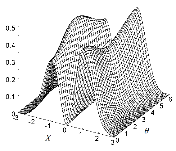
a)

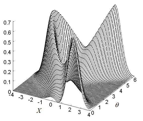
b)

Figure 1: Optical tomograms $w_{\alpha}(X,\theta)$ of photon-added coherent states for $\Omega(t)=1$, $m=1$, $\alpha=0.1$ (a), $\alpha=1$ (b).

3.2 Photon-added even/odd coherent states

Photon-added even/odd coherent states $|\alpha_{\pm},m\rangle$ were introduced in [4] as follows

$$|\alpha_{\pm},m\rangle=\frac{\hat{a}^{{\dagger}m}|\alpha_{\pm}\rangle}{(\langle\alpha_{\pm}|\hat{a}^{m}\hat{a}^{{\dagger}m}|\alpha_{\pm}\rangle)^{1/2}},$$ (20)

where $|\alpha_{\pm}\rangle$ is an even/odd coherent states [19], [27] and $m$ is an integer. The normalized states $|\alpha_{\pm}\rangle$ can be written as

$$|\alpha_{+}\rangle=\frac{e^{|\alpha|^{2}/2}}{2\sqrt{\cosh{|\alpha|^{2}}}}(|\alpha\rangle~{}+~{}|-\alpha\rangle),$$

$$|\alpha_{-}\rangle=\frac{e^{|\alpha|^{2}/2}}{2\sqrt{\sinh{|\alpha|^{2}}}}(|\alpha\rangle~{}-~{}|-\alpha\rangle).$$

Photon-added even/odd coherent states $|\alpha_{\pm},m\rangle$ in terms of photon-added coherent states $|\alpha,m\rangle$ are represented as follows [4]:

$$|\alpha_{\pm},m\rangle=\left(\frac{e^{|\alpha|^{2}}L_{m}(-|\alpha|^{2})}{2(e^{|\alpha|^{2}}L_{m}(-|\alpha|^{2})\pm e^{-|\alpha|^{2}}L_{m}(|\alpha|^{2}))}\right)^{1/2}~{}(|\alpha,m\rangle~{}\pm~{}|-\alpha,m\rangle)$$ (21)

This formula in view of (1) and (12) enables us to get the result

$$M_{\alpha_{\pm}m}(X,\mu,\nu,t) = \frac{e^{|\alpha|^{2}}L_{m}(-|\alpha|^{2})}{2(e^{|\alpha|^{2}}L_{m}(-|\alpha|^{2})\pm e^{-|\alpha|^{2}}L_{m}(|\alpha|^{2}))}$$ (22)

$$\times \left\{M_{\alpha m}(X,\mu,\nu,t)~{}+~{}M_{-\alpha m}(X,\mu,\nu,t)\right.$$

$$\pm \left.2\mbox{Re}~{}[\langle X,\mu,\nu|\alpha,m,t\rangle\langle-\alpha,m,t|X,\mu,\nu\rangle]\right\},$$

and with respect to (4) we have $w_{\alpha_{\pm}m}(X,\theta,t)=M_{\alpha_{\pm}m}(X,\mu=\cos\theta,\nu=\sin\theta,t)$, and in the case of stationary Hamiltonian with $\Omega(t)=1$ we have $w_{\alpha_{\pm}m}(X,\theta,t)=w_{\alpha_{\pm}m}(X,t+\theta)$.

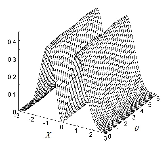
a)

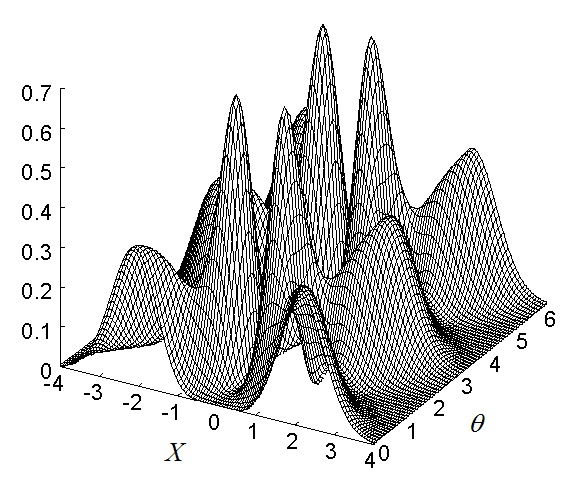
b)

Figure 2: Optical tomograms $w_{\alpha_{+}}(X,\theta)$ of even photon-added coherent states for $\Omega(t)=1$, $m=1$, $\alpha=0.1$ (a), $\alpha=1$ (b).

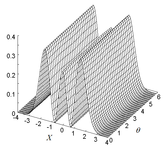
a)

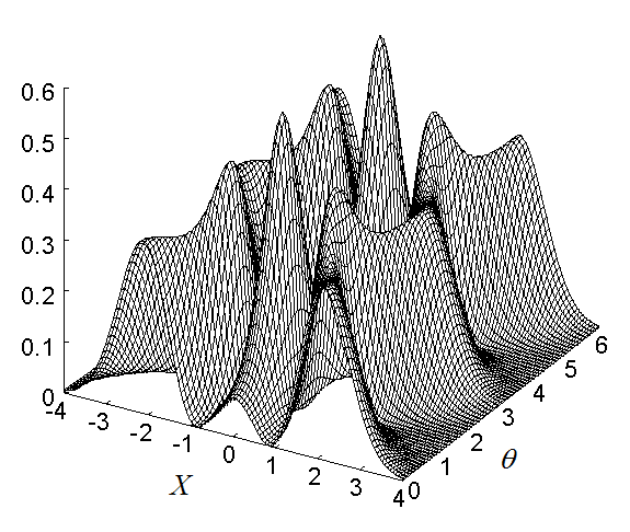
b)

Figure 3: Optical tomograms $w_{\alpha_{-}}(X,\theta)$ of odd photon-added coherent states for $\Omega(t)=1$, $m=1$, $\alpha=0.1$ (a), $\alpha=1$ (b).

3.3 Photon-added thermal states

A thermal state is the most classical state of light, formed by a statistical mixture of coherent states. The density operator of thermal state has the form $\hat{\rho}_{\rm T}=Z^{-1}e^{-\hat{H}/T}$, $Z={\rm Tr}e^{-\hat{H}/T}$. The associated optical tomogram reads $w_{\rm T}(X,\theta)=\displaystyle{\frac{1}{\sqrt{2\pi\sigma^{2}}}e^{-X^{2}/2\sigma^{2}}}$, where $\sigma^{2}=\frac{1}{2}\coth\frac{1}{2T}$. The density matrix of the photon-added thermal states in representation of the Fock states $|n,t\rangle$ is given by

$$\langle k,t|\hat{\rho}_{Tm}|n,t\rangle=\langle k,t|\hat{a}^{{\dagger}m}\hat{\rho}_{T}~{}\hat{a}^{m}|n,t\rangle=\delta_{kn}\frac{(1-e^{-1/T})^{m+1}}{m!}\frac{n!}{(n-m)!}e^{-(n-m)/T},~{}~{}~{}~{}(k,~{}~{}n\geq m).$$ (23)

The symplectic tomogram of this state can be written as follows

$$M_{Tm}(X,\mu,\nu,t)=\sum_{n=0}^{\infty}\langle n+m,t|\hat{\rho}_{Tm}|n+m,t\rangle|\langle X,\mu,\nu|n+m,t\rangle|^{2}.$$ (24)

Noting that $|\langle X,\mu,\nu|n,t\rangle|^{2}=M_{\alpha=0,n}(X,\mu,\nu,t)$, with the help of (18) we can find the result

$$M_{Tm}(X,\mu,\nu,t) = \frac{(1-e^{-1/T})^{m+1}}{\sqrt{\pi}~{}m!~{}2^{m}~{}|\mu\varepsilon+\nu\dot{\varepsilon}|}~{}e^{-X^{2}/|\mu\varepsilon+\nu\dot{\varepsilon}|^{2}}$$ (25)

$$\times \sum_{n=0}^{\infty}\frac{e^{-n/T}}{n!~{}2^{n}}~{}\left|H_{n+m}\left\{\frac{X\varepsilon}{|\varepsilon|(\mu\varepsilon+\nu\dot{\varepsilon})}\left(\frac{|\varepsilon|^{2}(\mu\varepsilon+\nu\dot{\varepsilon})}{\varepsilon^{2}(\mu\varepsilon^{*}+\nu\dot{\varepsilon}^{*})}\right)^{1/2}\right\}\right|^{2}.$$

For the stationary Hamiltonian the optical tomogram can be read

$$w_{Tm}(X,\theta)=\frac{(1-e^{-1/T})^{m+1}}{\sqrt{\pi}~{}m!~{}2^{m}}~{}e^{-X^{2}}\sum_{n=0}^{\infty}\frac{e^{-n/T}H_{n+m}^{2}(X)}{n!~{}2^{n}}.$$ (26)

Thus the optical tomogram of the photon-added thermal state for the stationary Hamiltonian is not depend on time and on the parameter $\theta$. This formula with the help of the known summing expression for Hermite polynomials [24]

$$(1-\eta^{2})^{-1/2}\exp\left(\frac{2xy\eta-(x^{2}+y^{2})\eta^{2}}{1-\eta^{2}}\right)=\sum_{n=0}^{\infty}\frac{H_{n}(x)H_{n}(y)}{2^{n}~{}n!}\eta^{n},$$

is transformed to the differential expression for $w_{Tm}(X,\theta)=w_{Tm}(X)$

$$w_{Tm}(X)=\frac{(1-e^{-1/T})^{m+1}}{\sqrt{\pi}~{}m!}e^{-X^{2}}\frac{\partial^{m}}{\partial\eta^{m}}\left(\frac{\exp\left(\frac{2X^{2}\eta}{1+\eta}\right)}{\sqrt{1-\eta^{2}}}\right)_{\eta=e^{-1/T}}.$$ (27)

It gives us for $m=1$ and $m=2$ the following relations:

$$w_{Tm=1}(X)=\frac{(1-e^{-1/T})^{2}}{\sqrt{\pi}\sqrt{1-e^{-2/T}}}~{}e^{-X^{2}\tanh{(1/2T)}}\left\{\frac{2X^{2}}{(1+e^{-1/T})^{2}}+\frac{e^{-1/T}}{1-e^{-2/T}}\right\};$$ (28)

$$w_{Tm=2}(X) = \frac{(1-e^{-1/T})^{3}}{2\sqrt{\pi}\sqrt{1-e^{-2/T}}}~{}e^{-X^{2}\tanh{(1/2T)}}$$ (29)

$$\times \left\{\frac{4X^{4}}{(1+e^{-1/T})^{4}}+\frac{4X^{2}(2e^{-1/T}-1)}{(1+e^{-1/T})^{2}(1-e^{-2/T})}+\frac{2e^{-2/T}+1}{(1-e^{-2/T})^{2}}\right\}.$$

In Figures 1 - 4 we illustrated tomograms of photon-added states for some examples.

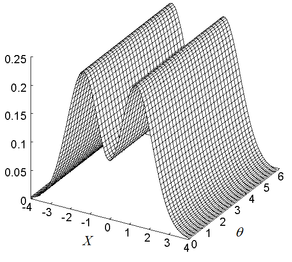
a)

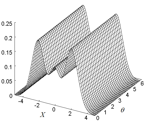
b)

Figure 4: Optical tomograms $w_{Tm}(X,\theta)$ of thermal states for $T=1$, $m=1$ (a), $m=2$ (b).

4 Conclusion

To resume we point out the main results of our paper. We calculated the optical tomograms of photon-added states. The initial states to which the photon are added are chosen as coherent state, thermal state, even and odd coherent state. We considered these states since they have been realized experimentally in [7],[8], [10] . We pointed out that the optical tomograms in probability representation of quantum mechanics can be considered as primary objects containing complete information on quantum states (see, e. g. [15]).

In view of this the reconstructing the Wigner function or Husimi function do not add extra information on the state property. Thus the problem is to measure the optical tomogram with highest possible accuracy. The precision of the experiments for measuring optical tomogram can be checked using such criteria as quadrature uncertainty relation with purity (temperature) dependent bound [28]. This criteria was suggested in [23] to control precision of the homodyne experiments. In the mentioned experimental works [7], [8], [9], [10], [11], including the homodyne two-mode studies [20] the checking correspondence to the above criteria has not been done. It is especially important, taking into account that the local oscillator phase contribution can influence the final results if the states under the study differ from the states (thermal or photon-added thermal) with optical tomograms not depending on the local oscillator phase.

It is of special interest to test the experimental optical tomogram in the sense that it must satisfy the discussed in introduction symmetry condition with respect to shift of local oscillator phase by $\pi$. In view of this we suggest to measure accurately the optical tomograms not only in domain of local oscillator phase $0\geq\theta\geq\pi$ but to investigate accurately also the domain $\pi\geq\theta\geq 2\pi$ to check the symmetry properties of the tomogram. Using the theoretically calculated optical homodyne probabilities as a standard for comparison with the experimental results, one can estimate measure of necessity of the precision improvement of the technique in future experiments.

5 Acknoledgments

V.I.M. thank the Russian Foundation for Basic Research for partial support under Projects Nos. 09-02-00142 and 10-02-00312.

References

- [1] V. V. Dodonov, J. Opt. B: Quantum Semiclass. Opt., 4, R1, (2002).
- [2] G.S.Agarwal, K.Tara, Phys. Rev. A, 492 (1991).
- [3] V. V. Dodonov, M. A. Marchiolli, Ya. A. Korennoy, V.I. Man’ko, E. A. Moukhin, Phys. Rev. A, 58, 4087 (1998).
- [4] V. V. Dodonov, Ya. A. Korennoy, V.I. Man’ko, E. A. Moukhin, J. Opt. B: Quantum Semiclass. Opt., 8, 413, (1996).
- [5] A. V. Dodonov, S. S. Mizrahi, Phys. Rev. A, 79, 023821 (1-7), (2009).
- [6] V. V. Dodonov, S. S. Mizrahi, J. Phys. A: Math. Gen., 35, 8847, (2002).
- [7] A.Zavatta, S. Vicinai, M. Bellini, Science, 306, 660, (2004).
- [8] V.Parigi, A.Zavatta, M. Kim, S. Vicinai, M. Bellini, Science, 317, 1890, (2007).
- [9] M. Barbieri, N. Spagnolo, M. G. Genoni, F. Ferreyrol, R. Blandino, M. G. A. Paris, P. Grangier, R. Tualle-Brouri, Phys. Rev. A, 82, 063833 (1-5), (2010).
- [10] A.Zavatta, V. Parigi, M. S. Kim, M. Bellini, Phys. Rev. Lett., 103, 140406, (2009).
- [11] T. Kiesel, W. Vogel, M.Bellini, A. Zavatta, Los Alamos arhiv, arXiv:1101.1741v1 [quant-ph] (2011).
- [12] D. T. Smithey, M. Beck, M. G. Raymer, A. Faridani, Phys. Rev. Lett., 70, 1244 (1993).
- [13] A. I. Lvovsky and M. G. Raymer, Rev. Mod. Phys., 81, 299 (2009).
- [14] S. Mancini, V. I. Man’ko, and P. Tombesi, Phys. Lett. A, 213, 1 (1996).
- [15] A. Ibort, V. I. Man’ko, G. Marmo, A. Simoni, and F. Ventriglia, Phys. Scr., 79, 065013 (2009).
- [16] D. Kalamidas, C. C. Gerry and A. Benmoussa, Phys. Lett. A,372, 1937, (2008).
- [17] M. Aspelmeyer, S. Groblacher, K. Hammerer and N. Kiesel, J. Opt. Soc. Am. B, 27, A189, (2010).
- [18] S. Sivakumar, Los Alamos arhiv, arXiv:1101.3855v1 [quant-ph] (2011).
- [19] V.V.Dodonov, I.A.Malkin, V.I.Man’ko,Physica, 72, 597 (1974).
- [20] C. Eicher, D. Bozyigit, C. Lang, M. Baur, L. Steffen, J. M. Fink, S. Filipp, A. Wallraff, Los Alamos arhiv, arXiv:1101.2136v1, [quant-ph], (2011).
- [21] G. M. D’Ariano, S. Mancini, V. I. Man’ko and P. Tombesi, J. Opt. B: Quantum Semiclass. Opt., 8, 1017 (1996).
- [22] Ya. A. Korennoy, V.I. Man’ko, Los Alamos arhiv, arXiv:1101.2537v1, [quant-ph], (2011).
- [23] V. I. Man’ko, G. Marmo, A. Porzio, S. Solimeno, and F. Ventriglia, “Homodyne extimation of quantum states purity by exploiting covariant uncertainty relation,” arXiv:1012.3297v1, [quant-ph], (2010).
- [24] Bateman Manuscript Project: Higher Transcendental Functions, edited by A. Erdélyi (McGraw-Hill, New York, 1953).
- [25] G. Szegö, Orthogonal Polynomials (American Mathematical Society, Providence, RI, 1959).
- [26] I.A.Malkin and V.I.Man’ko, Phys. Lett. A 31, 243 (1970).
- [27] N. A. Ansari, V. I. Manko, Phys. Rev. A, 50, 1942, (1994).
- [28] V. V. Dodonov, V. I. Manko, Proc. Lebedev Physical Institute, 183, 5, (1987).