Emerging Flux Simulations and Proto-Active Regions

Abstract

The emergence of minimally structured (uniform and horizontal) magnetic field from a depth of 20 Mm has been simulated. The field emerges first in a mixed polarity pepper and salt pattern, but then collects into separate, unipolar concentrations and produces pores. The field strength was then artificially increased to produce spot-like structures. The field strength at continuum optical depth unity peaks at 1 kG, with a maximum of 4 kG. Where the vertical field is strong, the spots persist (at present an hour of solar time has been simulated). Where the field is weak, the spot gets filled in and disappears. Stokes profiles have been calculated and processed with the Hinode annular mtf, the slit diffraction and frequency smoothing. These data are available at steinr.pa.msu.edu/$\sim$bob/stokes.

¹Michigan State University, East Lansing, MI 48824, USA

²Niels Bohr Institute, Blegdamsvej 17, 2100 Kobenhavn Ø, DK

1 Introduction

The rise of a coherent, straight, horizontal, twisted flux tube through the shallow layers of realistic solar convection zones has been studied by Cheung et al. (2008, 2007, 2006) and Martínez-Sykora et al. (2009, 2008). The structure of sunspots has been simulated by Rempel et al. (2009b, a) starting from an initial state of a coherent, vertical, cylindrical magnetic flux tube and by Cheung et al. (2010) for a buoyant, coherent, twisted, semi-torus flux tube kinematically advected into the domain from a depth of 7.5 Mm. We have investigated a complementary configuration where minimally structured, uniform, untwisted, horizontal field is advected into the computational domain by convective inflows through the bottom at a depth of 20 Mm. Earlier results were reported by Stein et al. (2010).

2 The Simulation

We use the “Stagger-Code”, which solves the equations for mass, momentum and internal energy in conservative form plus the induction equation for the magnetic field, for fully compressible flow, in three dimensions, on a staggered mesh. The dimensions are 48 Mm wide and extends from the temperature minimum at the top of the photosphere to a depth of 20 Mm (half the scale heights of the convection zone). The code uses finite differences, with 6th order derivative operators and 5th order interpolation operators. The grid is uniform and periodic in horizontal directions and non-uniform in the vertical (stratified) direction. Time integration is by a 3rd order low memory Runge-Kutta scheme (Kennedy et al. 1999). Parallelization is achieved with MPI, communicating the three overlap zones that are needed in the 6th and 5th order derivative and interpolation stencils. Horizontal directions are periodic. Top and bottom boundaries are transmitting. Inflows at the bottom boundary have uniform pressure, specified entropy and damped horizontal velocities. Outflow boundary values are obtained by extrapolation. The magnetic field is made to tend toward a potential field at the top and at the bottom is given a specified value in inflows and extrapolated in outflows.

We use a tabular equation of state that includes local thermodynamic equilibrium (LTE) ionization of the abundant elements as well as hydrogen molecule formation, to obtain the pressure and temperature as a function of log density and internal energy per unit mass. We calculate the radiative heat/cooling by solving the radiation transfer equation in both continua and lines using the Feautrier method (Feautrier 1964), assuming Local Thermodynamic Equilibrium (LTE). The number of wavelengths for which the transfer equation is solved is drastically reduced by using a multi-group method whereby the opacity at each wavelength is placed into one of four bins according to its magnitude and the source function is binned the same way (Nordlund 1982; Stein & Nordlund 2003; Vögler et al. 2004).

At supergranule and larger scales, the coriolis force of the solar rotation begins to influence the plasma motions, so f-plane rotation is included in the simulation. Angular momentum conservation produces a surface shear layer with the surface (top of the domain) rotating slower than the bottom of the domain, as observed in the Sun.

The simulation is started from a snapshot of hydrodynamic convection and inflows at the bottom (20 Mm depth) advect in uniform, untwisted, horizontal field.

3 Emerging Flux

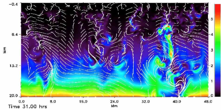
Figure 1.: Magnetic field (color) advected through the bottom boundary by inflows, rising through the upper convection zone. The plasma flow (white arrows) advects the field toward the surface in upflows and inhibits its rise in downflows. Scale is in kG.

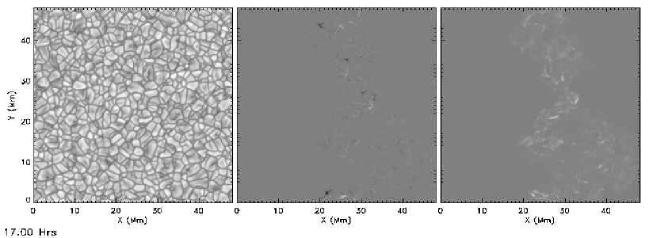
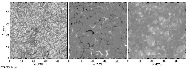
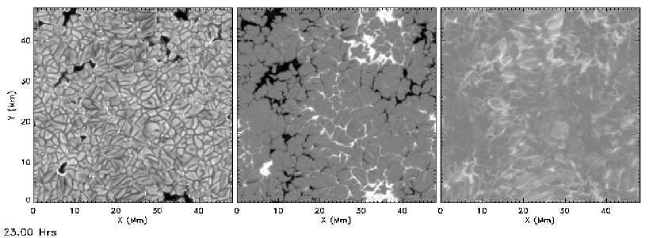
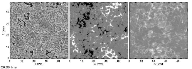
Figure 2.: Emergent continuum intensity (left), vertical magnetic field at $\tau_{\rm cont}=0.01$ (center) and horizontal magnetic field at the same optical depth (right). The range of intensities is 0.22-1.35$<I>$. The range of magnetic field is $\pm 2$ kG. Time is since horizontal field started entering at 20 Mm depth. The typical fluid rise time is 32 hours from that depth.

Upflows, aided by magnetic buoyancy, carry the magnetic flux to the surface. Downflows tend to pin the field down (Fig. 1). This results in the development of magnetic loops. The typical time for fluid to rise from a depth of 20 Mm to the surface is 32 hours. In the present case of 20 kG field at 20 Mm depth, the magnetic flux reaches the surface in approximately 20 hours. Magnetic flux initially appears in a small localized portion of the surface, but quickly spreads to cover the entire surface in a pepper and salt pattern of mixed polarity. The different polarities then collect into unipolar regions (Fig. 2). The small scale convective motions near the surface produce small serpentine loops that ride piggy-back on the larger loops produced by supergranule scale convective motions at large depths (Fig. 3).

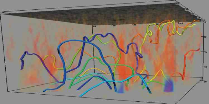
Figure 3.: Several magnetic field lines show large scale loops with smaller serpentine loops riding piggy-back on them. Shading shows downflows.

4 Active Region

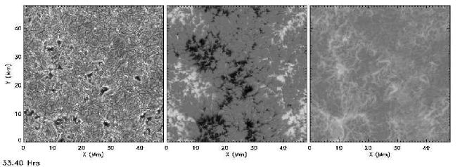
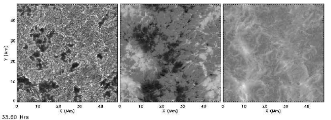
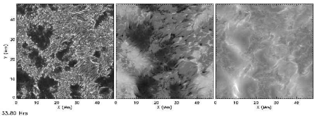
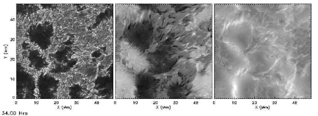
Figure 4.: Time sequence showing how the active region is produced by increasing the magnetic field strength $\propto B$. Emergent continuum intensity (left), vertical magnetic field at $\tau_{\rm cont}=0.01$ (center) and horizontal magnetic field at the same optical depth (right). The range of intensities is 0.15-2$<I>$. The range of magnetic field is $\pm 3$ kG. Time is since the start of horizontal field being advected into the 20 Mm deep domain.

Once sufficient magnetic flux had arrived at the surface (Fig. 2), we artificially increased the magnetic field strength, in proportion to its existing strength, with a time scale of 30 minutes (Fig. 4). This made the area occupied by the strong fields and the pores they had produced increase. However, the field strength at a fixed optical depth increased only slightly as the Wilson depression deepened and the surrounding gas pressure at fixed optical depth in the flux concentration increased. This method of simulating an active region allows the magnetic structures to develop naturally in magneto-convection before their strength is increased to produce the large magnetic fluxes associated with pores and sunspots, rather than imposing a given geometry to begin with.

There are very strong horizontal fields, in low lying loops, connecting the opposite polarity field concentrations because of the close proximity of the opposite polarity regions. This produces elongated granules and penumbral-like features, but the crowding does not allow them to grow as in observed sunspots.

The active region, so far, has evolved for 2 hours. During this time the areas of strong vertical field concentrations have maintained their integrity (Fig. 5: yellow and dark blue contours are vertical magnetic field $\pm$ 2 kG and red and green are $\pm$ 2.5 kG). Areas with weaker vertical field have gotten filled in by convective plumes from their periphery plunging into their interior and dispersing the magnetic field into small, isolated clumps (See region in the center-right of Fig. 5 compared with the same region in the very center of Fig. 4 at an earlier time).

Figures 6 and 7 are more detailed images of the spots in the lower left and top center of Fig. 5, but at a slightly earlier time. The short light bridge in Fig. 6 has the dark center lane and segmented appearance of observed light bridges. To the upper left in Fig. 6 there are strong shearing motions between the elongated granules. There is a very bright region on the left edge of the spot in Fig. 6 where there is a very strong vertical field concentration (see Fig. 5).

Figure 5.: Emergent continuum intensity image of simulated active region with vertical magnetic field contours at $\pm$ 2 (yellow and blue), $\pm$ 2.5 (red and green) kG.

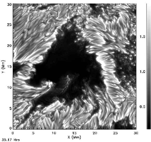
Figure 6.: Spot at lower left corner: emergent continuum intensity I/$<$I$>$.

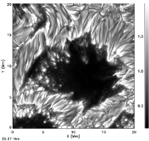
Figure 7.: Spot at top center: emergent continuum intensity I/$<$I$>$.

5 Stokes Profiles

In the centers of the pores/spots, the stokes profiles after passing through the Hinode optical path (as represented by the 50 cm annular psf, the slit diffraction and the 24 mÅ frequency smoothing) are identical to the profiles from the individual simulation pixels (24 km resolution). However, in the penumbral like features bordering the pores/spots, where the magnetic field is predominantly horizontal and the field, thermodynamic and velocity structures have small scale variations, the modified profiles are significantly different from individual pixel profiles (Fig. 8). Raw data, stokes profiles I,Q,U,V and profiles as modified by the Hinode optical path are available on line at http://steinr.pa.msu.edu/$\sim$bob/Stokes.

Figure 8.: Stokes V profiles for Fe I 630.15 and 630.25 nm lines for a penumbral region of a simulated spot: Original profile (solid line), neighboring profiles (dotted lines) and profile after Hinode mtf, slit diffraction and frequency smoothing (dashed line).

6 Comparison with Hinode Observations

In addition to the active region simulation described above, we also have performed a simulation with an initial uniform vertical magnetic field imposed on a snapshot of hydrodynamic convection. This calculation is being performed on a domain 12 Mm wide by 6 Mm deep. (There is no point to going deeper on such a narrow domain because the convective cells would become artificially constrained at larger depths by the periodic horizontal boundary conditions.) The vertical field was initial 10 G and was increased with a time scale of 2 hours. We have compared the emergent continuum intensity and vertical velocity from both the active region simulation and this vertical field simulation at the time when the average vertical field was 60 G, with observations from Hinode that were provided by Reza Rezaei (Figs. 9 and 10).

For the weak vertical field unipolar region compared to the quiet Sun observations, the raw simulation distribution of both intensity and velocity is much wider than observed. However, when the Hinode MTF is applied to the simulation results there is excellent agreement with the observations. For the active region simulation, on the other hand, agreement is not so good. The simulation results have much larger downward velocities and a larger fraction of both high and low intensities. The larger fraction of low intensities is due to the crowding of the dark spot-like areas. The origin of the much brighter locations is unclear. Figs. 6 and 7 show some very bright edges to the magnetic concentrations where the horizontal field turns over into vertical field.

Figure 9.: Emergent continuum intensity distribution, comparing simulation results and Hinode observations, for an active region (left) and quiet Sun (right).

Figure 10.: Vertical velocity distribution, comparing simulation results and Hinode observations, for an active region (left) and quiet Sun (right). Negative velocities are upward and positive velocities are downward.

Acknowledgments

This work was funded by NSF grant AST 0605738 and NASA grants NNX07AO71G, NNX07AH79G and NNX08AH44G. The calculations were performed on the Pleiades supercomputer of the NASA Advanced Supercomputing Division. It would not have been possible without this support.

References

- Cheung et al. (2006) Cheung, M. C. M., Moreno-Insertis, F., & Schüssler, M. 2006, A&A, 451, 303
- Cheung et al. (2010) Cheung, M. C. M., Rempel, M., Title, A. M., & Schüssler, M. 2010, ApJ, 720, 233
- Cheung et al. (2007) Cheung, M. C. M., Schüssler, M., & Moreno-Insertis, F. 2007, A&A, 467, 703. arXiv:astro-ph/0702666
- Cheung et al. (2008) Cheung, M. C. M., Schüssler, M., Tarbell, T. D., & Title, A. M. 2008, ApJ, 687, 1373. 0810.5723
- Feautrier (1964) Feautrier, P. 1964, SAO Special Report, 167, 80
- Kennedy et al. (1999) Kennedy, Carpenter, & Lewis 1999, ICASE Report, 99-22, 1
- Martínez-Sykora et al. (2008) Martínez-Sykora, J., Hansteen, V., & Carlsson, M. 2008, ApJ, 679, 871. 0712.3854
- Martínez-Sykora et al. (2009) — 2009, ApJ, 702, 129. 0906.5464
- Nordlund (1982) Nordlund, A. 1982, A&A, 107, 1
- Rempel et al. (2009a) Rempel, M., Schüssler, M., Cameron, R. H., & Knölker, M. 2009a, Science, 325, 171
- Rempel et al. (2009b) Rempel, M., Schüssler, M., & Knölker, M. 2009b, ApJ, 691, 640
- Stein et al. (2010) Stein, R. F., Lagerfjärd, A., Nordlund, Å., & Georgobiani, D. 2010, Solar Phys., 34
- Stein & Nordlund (2003) Stein, R. F., & Nordlund, Å. 2003, in Stellar Atmosphere Modeling, edited by I. Hubeny, D. Mihalas, & K. Werner, vol. 288 of Astronomical Society of the Pacific Conference Series, 519
- Vögler et al. (2004) Vögler, A., Bruls, J. H. M. J., & Schüssler, M. 2004, A&A, 421, 741