Quark-antiquark potential to order $1/m$
and heavy quark masses

Abstract

An updated heavy quark-antiquark potential is constructed by matching the short-distance perturbative part to long-distance lattice QCD results at an intermediate $r$ scale. The static potential and the order $1/m$ potential are both analyzed in this way. Effects of order $1/m$ in charmonium and bottomonium spectra are discussed in comparison. Charm and bottom quark masses are deduced from the spectra and related to the quark masses of other schemes.

I Introduction

Investigations of the potential between a heavy quark and its antiquark have a long tradition. Early models featuring the basic Coulomb-plus-linear $r$ dependence plus a hyperfine interaction established a quite successful phenomenology of charmonium spectroscopy below the open charm threshold. At short distances perturbative QCD is supposed to work. At larger distances lattice QCD results have confirmed the linearly rising confinement potential and established reliable values of the string tension.

It has long been realized that the static quarkonium potential, constructed within the framework of QCD perturbation theory, has a badly convergent or even divergent behavior at short distances. This has been understood in terms of renormalon ambiguities. It has in fact been found that leading renormalon effects cancel in the sum of the static potential and twice the quark (pole) mass Beneke:1998rk ; Hoang:1998nz , an important feature to be recalled later when we address the issue of quark masses in the context of the quarkonium potential and spectroscopy.

The steadily increasing precision of current lattice QCD computations permits now an accurate matching of perturbative and non-perturbative approaches at an intermediate distance scale. An update of this procedure, combined with an accurate analysis of charm and bottom quark masses, is the main topic of the present work.

This paper is organized as follows. After a brief summary of first attempts in Section II, the perturbative static potential in coordinate space and its overall additive constant are derived in Section III and matched at an appropriate distance scale with results from lattice QCD. Section IV follows with an analogous construction for the potential at order $1/m$ in the quark mass. Section V discusses $1/m$ effects on bottomonium and charmonium spectra. In the last section charm and bottom quark masses are deduced and compared with existing determinations in other schemes.

II Preparations

As a starting point, consider the static quark-antiquark potential in momentum space at three-loop order:

$$\tilde{V}^{(0)}(|\vec{q}\,|)=-\frac{4\pi C_{F}\alpha_{s}(|\vec{q}\,|)}{\vec{q}\,^{2}}\,\bigg{\{}1+\frac{\alpha_{s}(|\vec{q}\,|)}{4\pi}\,a_{1}+\left(\frac{\alpha_{s}(|\vec{q}\,|)}{4\pi}\right)^{2}a_{2}\\ +\left(\frac{\alpha_{s}(|\vec{q}\,|)}{4\pi}\right)^{3}\left(a_{3}+8\pi^{2}C_{A}^{3}\ln\frac{\mu_{\scriptscriptstyle\text{IR}}^{2}}{\vec{q}\,^{2}}\right)+\mathcal{O}\left(\alpha_{s}^{4}\right)\bigg{\}}\,,$$ (1)

where $\vec{q}$ is the three-momentum transfer. The coefficients $a_{1}$ and $a_{2}$ have been determined analytically and they read in the $\overline{\text{MS}}$ scheme Peter:1996ig ; Peter:1997me ; Schroder:1998vy :

$$a_{1} =\frac{31}{9}C_{A}-\frac{20}{9}T_{F}n_{f},$$ (2)

$$a_{2} =\left(\frac{4343}{162}+4\pi^{2}-\frac{\pi^{4}}{4}+\frac{22}{3}\zeta(3)\right)C_{A}^{2}-\left(\frac{1798}{81}+\frac{56}{3}\zeta(3)\right)C_{A}T_{F}n_{f}$$

$$\hskip 20.00003pt-\left(\frac{55}{3}-16\zeta(3)\right)C_{F}T_{F}n_{f}+\left(\frac{20}{9}T_{F}n_{f}\right)^{2},$$ (3)

where $C_{F}=4/3$, $C_{A}=3$, $T_{F}=1/2$ for SU(3) and $n_{f}$ is the number of light quark flavors. At three-loop order, infrared singular contributions $\ln(\mu_{\scriptscriptstyle\text{IR}}^{2}/\vec{q}\,^{2})$ start to play a role (see e.g. Brambilla:1999qa ). The accompanying constant

$$a_{3}=4^{3}\,(209.884(1)-51.4048n_{f}+2.9061n_{f}^{2}-0.0214n_{f}^{3})$$ (4)

has been calculated independently in Smirnov:2009fh and Anzai:2009tm . In this paper we focus on the two-loop level. In order to transform the potential to coordinate space, $\alpha_{s}(|\vec{q}\,|)$ in Eq. (1) is usually expressed (see e.g. Kniehl:2002br ) as a powers series expansion in $\alpha_{s}$ at some fixed scale $\mu$:

$$\alpha_{s}(q)=\alpha_{s}(\mu)\bigg{[}1 -\frac{\alpha_{s}(\mu)}{4\pi}\beta_{0}\,\ell+\left(\frac{\alpha_{s}(\mu)}{4\pi}\right)^{2}(\beta_{0}^{2}\,\ell\!-\!\beta_{1})\,\ell$$

$$+\left(\frac{\alpha_{s}(\mu)}{4\pi}\right)^{3}\left(-\beta_{0}^{3}\,\ell^{2}\!+\!\frac{5}{2}\beta_{0}\beta_{1}\,\ell\!-\!\beta_{2}\right)\ell$$

$$+\left(\frac{\alpha_{s}(\mu)}{4\pi}\right)^{4}\bigg{(}\beta_{0}^{4}\,\ell^{3}\!-\!\frac{13}{3}\beta_{0}^{2}\beta_{1}\,\ell^{2}\!+\!3\Big{(}\beta_{0}\beta_{2}\!+\!\frac{\beta_{1}^{2}}{2}\Big{)}\ell\!-\!\beta_{3}\bigg{)}\ell+\mathcal{O}\left(\alpha_{s}^{5}\right)\bigg{]},$$ (5)

with $\ell=\ln(q^{2}/\mu^{2})$. The coefficients $\beta_{n}$ of the QCD $\beta$ function are known up to four-loop order vanRitbergen:1997va :

$$\frac{\partial\alpha_{s}(\mu)}{\partial\ln\mu^{2}}=\beta(\alpha_{s})=-\frac{\alpha_{s}^{2}}{4\pi}\beta_{0}-\frac{\alpha_{s}^{3}}{(4\pi)^{2}}\beta_{1}-\frac{\alpha_{s}^{4}}{(4\pi)^{3}}\beta_{2}-\frac{\alpha_{s}^{5}}{(4\pi)^{4}}\beta_{3}+\mathcal{O}(\alpha_{s}^{6}).$$ (6)

In this approach a Fourier transform leads to the standard, $\mu$-dependent definition of the coordinate space static potential,

$$V^{(0)}(r)=-\frac{4\,\alpha_{s}(\mu)}{3\,r}\,\bigg{\{}1+\frac{\alpha_{s}(\mu)}{4\pi}\,\Big{[}a_{1}+2\beta_{0}\,g_{\mu}(r)\Big{]}\\ +\bigg{(}\frac{\alpha_{s}(\mu)}{4\pi}\bigg{)}^{2}\Big{[}a_{2}+\beta_{0}^{2}\big{(}4g_{\mu}^{2}(r)\!+\!\pi^{2}/3\big{)}+2g_{\mu}(r)(2a_{1}\beta_{0}\!+\!\beta_{1})\Big{]}\\ +\bigg{(}\frac{\alpha_{s}(\mu)}{4\pi}\bigg{)}^{3}\Big{[}a_{3}+16\pi^{2}C_{A}^{3}\big{(}\ln(\mu_{\scriptscriptstyle\text{IR}}r)\!+\!\gamma_{\scriptscriptstyle\text{E}}\big{)}+\beta_{0}^{3}\big{(}8g_{\mu}^{3}(r)\!+\!2\pi^{2}g_{\mu}(r)\!+\!16\zeta(3)\big{)}\\ +\beta_{0}\big{(}12g_{\mu}^{2}(r)\!+\!\pi^{2}\big{)}\big{(}a_{1}\beta_{0}\!+\!5/6\,\beta_{1}\big{)}+2g_{\mu}(r)\big{(}3a_{2}\beta_{0}\!+\!2a_{1}\beta_{1}\!+\!\beta_{2}\big{)}\Big{]}+\mathcal{O}(\alpha_{s}^{4})\bigg{\}}\,,$$ (7)

where $g_{\mu}(r)=\ln(\mu r)+\gamma_{\scriptscriptstyle\text{E}}\,$. The derivation of this $r$-space potential uses, in principle, information about $\alpha_{s}(|\vec{q}\,|)$ over the full range in $q$ space.

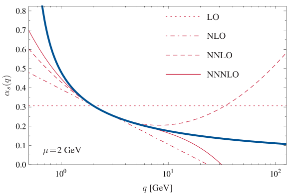
Figure 1: Power series expansion of $\alpha_{s}(q)$ at $\mu\!=\!2$ GeV for $n_{f}\!=\!4$. The thick line shows the full four-loop running according to the renormalization group equation. Note that the sign of $\alpha_{s}(q\to\infty)$ changes order by order.

However, the expansion (II) in powers of $\ln q^{2}$ is a good approximation only in a small neighborhood of the scale $\mu$, as demonstrated in Fig. 1 for the choice $\mu=2$ GeV. Clearly, the behavior of $\alpha_{s}(q)$ for $q>10$ GeV and $q<1$ GeV is out of control for such an expansion.

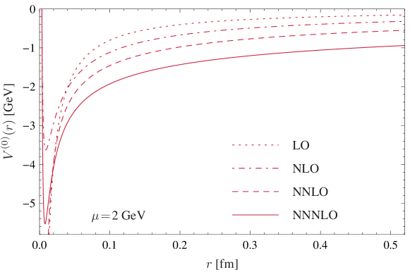
Figure 2: Static $r$-space potential according to Eq. (7) using $\mu\!=\!2$ GeV. The choice $\mu_{\scriptscriptstyle\text{IR}}^{2}\!=\!\vec{q}\,^{2}$ has been adopted at NNNLO.

Fixing $\mu$ for instance at 2 GeV, the resulting coordinate space potential (7) behaves pathologically at $r\!\to\!0$, as shown in Fig. 2. This behavior can be traced to the order-by-order sign changes observed in Fig. 1 for $q\!\to\!\infty$. It can be improved using the renormalon subtracted scheme (see e.g. Pineda:2002se ; Brambilla:2009bi ).

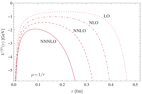
Figure 3: Static $r$-space potential according to Eq. (7). Progressive orders are shown when $\mu$ is identified with $1/r$. The choice $\mu_{\scriptscriptstyle\text{IR}}^{2}\!=\!\vec{q}\,^{2}$ has been adopted at NNNLO.

Figure 3 shows the potential resulting from the frequently used ad hoc identification $\mu=1/r$ which evidently works only at extremely short distances, $r<0.02$ fm. Such a construction therefore does not suggest itself for a matching of the potential to lattice QCD results at typical distances $r\gtrsim 0.1$ fm.

III The static potential

Here we pursue a different strategy for constructing the static potential in coordinate space, based on the potential-subtracted (PS) scheme proposed by Beneke Beneke:1998rk . The $r$-space potential is defined through a restricted Fourier transform as

$$V^{(0)}(r,\mu_{f})=\intop_{|\vec{q}\,|>\mu_{f}}\!\!\frac{d^{3}q}{(2\pi)^{3}}\ e^{i\vec{q}\cdot\vec{r}}\,\tilde{V}^{(0)}(|\vec{q}\,|)\,,$$ (8)

where $\tilde{V}^{(0)}(|\vec{q}\,|)$ is given in Eq. (1), but now $\alpha_{s}(|\vec{q}\,|)$ for $|\vec{q}\,|>\mu_{f}$ is used without resorting to a power series expansion. The momentum space cutoff $\mu_{f}$ is introduced in order to delineate the uncontrolled low-$q$ region from the high-$q$ range where perturbation theory is considered to be reliable. The potential (8) differs from the “true” static potential,

$$V^{(0)}(r)=v^{(0)}(\mu_{f})+V^{(0)}(r,\mu_{f})\,,$$ (9)

approximately by a constant,

$$v^{(0)}(\mu_{f})=\intop_{|\vec{q}\,|\leq\mu_{f}}\!\!\frac{d^{3}q}{(2\pi)^{3}}\ e^{i\vec{q}\cdot\vec{r}}\,\tilde{V}^{(0)}(|\vec{q}\,|)=\frac{1}{2\pi^{2}}\intop_{0}^{\mu_{f}}\!dq\,q^{2}\,\tilde{V}^{(0)}(q)+\mathcal{O}(\mu_{f}^{2}\,r^{2})\,,$$ (10)

which encodes non-perturbative low-$q$ behavior that can be absorbed in the definition of the potential-subtracted (PS) quark mass (see Section VI). The correction of order $\mu_{f}^{2}\,r^{2}$ is negligibly small in the range of interest ($r<0.1$ fm).

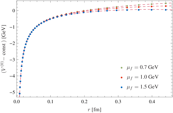
Figure 4: Static QCD potential (with $n_{f}=3$) from the restricted numerical Fourier transform (8). Shown is the NNLO potential for different values of $\mu_{f}$. The curves have been shifted by a constant to match at small $r$ values.

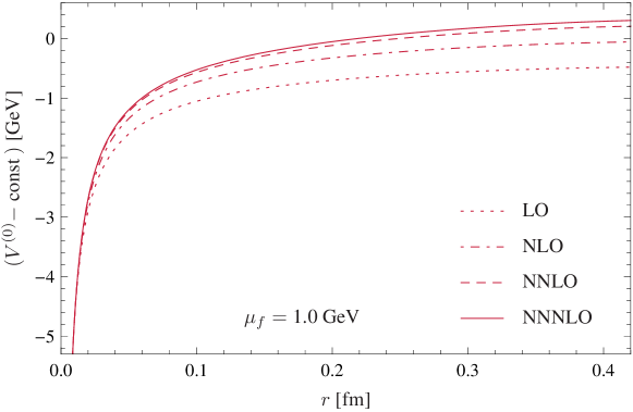
Figure 5: Static QCD potential (with $n_{f}=3$ and $\mu_{f}\!=\!1.0$ GeV) from the restricted numerical Fourier transform (8). Different orders of have been matched at $0.01$ fm. The choice $\mu_{\scriptscriptstyle\text{IR}}^{2}\!=\!\vec{q}\,^{2}$ has been adopted at NNNLO.

The potential $V^{(0)}(r,\mu_{f})$ is evaluated numerically using the four-loop renormalization group running of the strong coupling $\alpha_{s}$, see Eq. (6). For distances $r<0.2$ fm, the resulting potential depends only marginally on $\mu_{f}$ as shown in Fig. 4. At the matching radius, $r=0.14$ fm, the spread of $(V^{(0)}-\text{const})$ when varying $\mu_{f}$ between $0.7$ GeV and $1.5$ GeV is $0.05$ GeV. The convergence behavior of the potential is displayed in Fig. 5. Different orders have been matched at $r=0.01$ fm and are then evolved to larger distances. Evidently, the convergence behavior of the potential $V^{(0)}(r,\mu_{f})$ is satisfactory.

For bottomonium ($n_{f}\!=\!4$ massless flavors), the input value for the renormalization group running of the strong coupling constant is chosen as $\alpha_{s}(4.2\ \text{GeV})=0.226\pm 0.003$. In the case of charmonium ($n_{f}\!=\!3$) we use $\alpha_{s}(1.25\ \text{GeV})=0.406\pm 0.010$ as input in the potential. These values are obtained from $\alpha_{s}(m_{Z}\!=\!91.1876\ \text{GeV})=0.1184\pm 0.0007$ Bethke:2009jm (for a theory with $n_{f}\!=\!5$ active quark flavors) and run down to $4.2$ GeV and $1.25$ GeV, taking into account flavor thresholds Chetyrkin:1997sg .

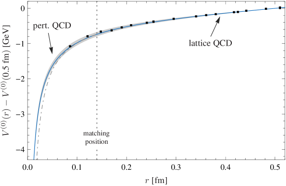
Figure 6: Static QCD potential for $n_{f}=3$, based on Eqs. (8) and (1), matched at intermediate distances to a potential from lattice QCD Bali:2000vr . Dashed-dotted curve: simplest extrapolation using Coulomb-plus-linear $r$ dependence.

The perturbative potential (8), valid at small distances, can be matched at intermediate distances to results from lattice QCD (see Fig. 6). We use a fit obtained by Bali et al. from a full QCD simulation Bali:2000vr . The matching point (dashed line) is chosen at $r=0.14$ fm. The exact position of the matching point is not important for the resulting shape of the potential. At $r=0.14$ fm, both the perturbative and the lattice potential are expected to be reliable. Requiring that the first derivative of the potential is continuous at the matching point, we find for the cutoff in Eq. (8): $\mu_{f}=0.908$ GeV (bottomonium case) and $\mu_{f}=0.930$ GeV (charmonium case). The grey band reflects uncertainties in the Sommer scale $r_{0}=0.50\pm 0.03$ fm (lattice part) and uncertainties in $\alpha_{s}(|\vec{q}\,|)$ (perturbative part) as given in the previous paragraph. This leads to a cutoff window: $\mu_{f}=0.9^{+0.3}_{-0.2}$ GeV (for both bottomonium and charmonium). The dashed-dotted line in Fig. 6 results from a simple Coulomb-plus-linear extrapolation from the lattice QCD data to short distances. Evidently, our more sophisticated perturbative QCD extrapolation based on Eqs. (8) and (1) differs from that simple form.

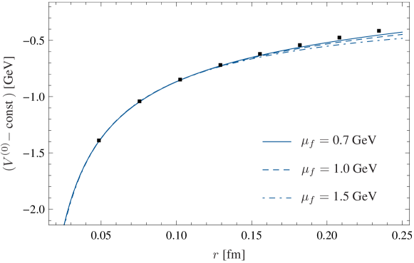
Figure 7: The static potential for $n_{f}\!=\!0$ flavors compared to lattice points Necco:2001xg . The lattice scale $r_{0}$ has been set to $0.5$ fm.

For zero flavors one can check against accurate (quenched) lattice results Necco:2001xg (see Fig. 7). Since $\alpha_{s}$ cannot be extracted from experiment for $n_{f}\!=\!0$, we fit to the lattice points below $0.12$ fm. With a low momentum cutoff $\mu_{f}$ in the range $0.7$–$1.5$ GeV, we find $\alpha_{s}(1.25\ \text{GeV})=0.29\pm 0.01$ for the flavorless strong coupling at the scale of the c-quark mass. The lattice scale $r_{0}=0.5$ fm has been used here. A recent precision study of the zero-flavor case in a different approach can be found in Ref. Brambilla:2010pp .

IV Order $1/m$ potential

The heavy quark-antiquark potential can be expanded in inverse powers of the heavy quark mass $m$:

$$V(r)=V^{(0)}(r)+\frac{V^{(1)}(r)}{m/2}+\frac{V^{(2)}(r)}{(m/2)^{2}}+\mathcal{O}(1/m^{3})\,.$$ (11)

The perturbative potential at order $1/m$ in momentum space reads:

$$\tilde{V}^{(1)}(|\vec{q}\,|)=\frac{C_{F}\,\pi^{2}\,\alpha_{s}^{2}(|\vec{q}\,|)}{2\,|\vec{q}\,|}\big{\{}-C_{A}+\mathcal{O}(\alpha_{s})\big{\}}\,,$$ (12)

with $C_{F}=4/3$ and $C_{A}=3$. This form is not unique, see Ref. Brambilla:2000gk , but we stick to the same convention as the one used on the lattice. $\tilde{V}^{(1)}(|\vec{q}\,|)$ can be transformed to $r$ space as in Eq. (8), with a low momentum cutoff $\mu^{\prime}_{f}$ that may differ from $\mu_{f}$:

$$V^{(1)}(r,\mu^{\prime}_{f})=\intop_{|\vec{q}\,|>\mu^{\prime}_{f}}\!\!\frac{d^{3}q}{(2\pi)^{3}}\ e^{i\vec{q}\cdot\vec{r}}\,\tilde{V}^{(1)}(|\vec{q}\,|)\,.$$ (13)

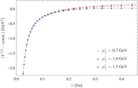
Figure 8: The order $1/m$ potential $V^{(1)}(r,\mu_{f}^{\prime})$ with $n_{f}=3$ from the restricted numerical Fourier transform (13), for different cutoffs $\mu^{\prime}_{f}$. The curves have been shifted by a constant to match at small $r$ values.

Evidently, the dependence of $V^{(1)}$ on the cutoff scale $\mu^{\prime}_{f}$ is again very weak for distances $r<0.2$ fm as shown in Fig. 8. The variation of $(V^{(1)}-\text{const})$ when varying $\mu^{\prime}_{f}$ between $0.7$ GeV and $1.5$ GeV is within $0.02$ GeV² at the matching radius, $r=0.14$ fm. This potential is again matched to corresponding results from lattice QCD Koma:2006si ; Koma:confinement8 . In order to fit the lattice data we have used

$$V^{(1)}_{\text{fit}}(r)=-\frac{c^{\prime}}{r^{2}}+d^{\prime}\ln\Big{(}\frac{r}{r_{0}}\Big{)}+\text{const}\,,$$ (14)

with $c^{\prime}\!=\!0.0027$ GeV${}^{2}\,$fm², $d^{\prime}\!=\!0.075$ GeV² and an arbitrary length scale $r_{0}$ that can be absorbed in the overall constant. The logarithmic form in Eq. (14) is motivated by effective string theory PerezNadal:2008vm . This parametrization extrapolates the lattice points for $V^{(1)}$ better than just a $1/r^{2}\,+\,$linear form. The lattice calculation of $V^{(1)}$ is quenched and subject to renormalization issues. A $15\%$ uncertainty is therefore assumed in the lattice potential, in addition to the uncertainties in the Sommer scale $r_{0}$.

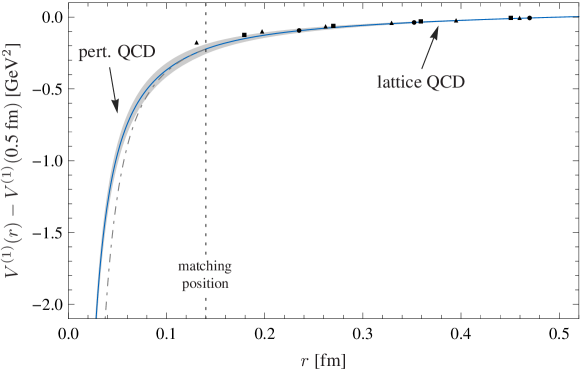
Figure 9: The order $1/m$ potential $V^{(1)}(r,\mu_{f}^{\prime})$ with $n_{f}=3$, based on Eq. (13), matched at intermediate distances to a potential from lattice QCD Koma:confinement8 . The fit and the matching has been performed using the lattice QCD points with $\beta\!=\!5.85$ (circles). Legends are analogous to Fig. 6. Dashed-dotted curve: simple extrapolation using Eq. (14).

At short distances a deviation of the perturbative potential $V^{(1)}(r,\mu^{\prime}_{f})$ from $V^{(1)}_{\text{fit}}$ of Eq. (14) (dashed-dotted line in Fig. 9) is apparent. For the cutoff in Eq. (13) with error estimate we find: $\mu^{\prime}_{f}=1.9^{+0.4}_{-0.6}$ GeV (bottomonium case) and $\mu^{\prime}_{f}=1.6^{+0.5}_{-0.8}$ GeV (charmonium case).

V Quarkonium spectra

Given the potential $V=V^{(0)}+2\,V^{(1)}/m$ up to order $1/m$ in the heavy quark mass, we can now examine the resulting bottomonium and charmonium spectra, with focus on the effects of the $1/m$ term. The Schrödinger equation

$$\bigg{[}-\frac{\hbar^{2}}{m}\vec{\nabla}^{2}+2m_{\widehat{\text{PS}}}(\mu_{f},\mu^{\prime}_{f})+V^{(0)}(r,\mu_{f})+\frac{2}{m}V^{(1)}(r,\mu^{\prime}_{f})-E\bigg{]}\psi(\vec{r}\,)=0\,,$$ (15)

is solved with the fixed values for $\mu_{f}$ and $\mu^{\prime}_{f}$ as derived in the construction of the potentials. The potential-subtracted mass $m_{\widehat{\text{PS}}}(\mu_{f},\mu^{\prime}_{f})$, to be defined and discussed in detail in Section VI, is the only free parameter. It sets the overall energy scale and it is ultimately fixed by comparison with the measured bottomonium and charmonium spectrum.

The (heavy) quark mass is not directly measurable. The mass $m$ appearing in the denominator of the kinetic energy and the $V^{(1)}$ term is therefore not a priori determined. In practice we use values close to the static $\overline{\text{MS}}$ masses: $m\!=\!4.2$ GeV for bottomonium and $m\!=\!1.25$ GeV for charmonium. Small variations from these values do not have any significant influence on the results.

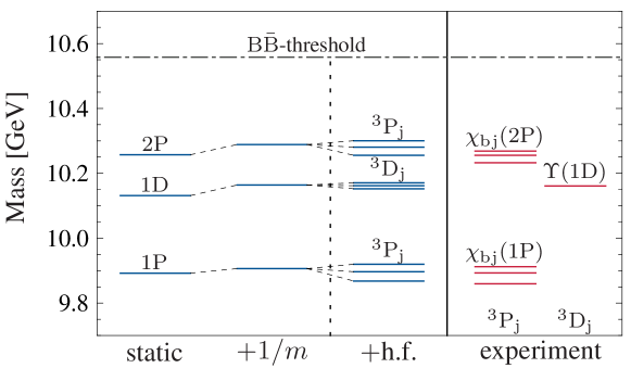
Figure 10: Bottomonium spectrum in comparison with experiment. Static plus order $1/m$ results are shown on the left, with additional hyperfine effects (h.f.) added phenomenologically using Eq. (16).

Consider now first the bottomonium spectrum below $\text{B}\overline{\text{B}}$ threshold (see Fig. 10). One can start by fixing $m_{\widehat{\text{PS}}}(\mu_{f},\mu^{\prime}_{f})$ such that the measured $\Upsilon\text{(2S)}$ energy is reproduced. Alternatively, the center of the $\chi_{\text{b}}\text{(1P)}$ triplet can be used for calibration. These states remain almost unchanged by the $1/m$ effects. The more tightly bound $\eta_{\text{b}}\text{(1S)}$ and $\Upsilon\text{(1S)}$ states respond, as expected, more sensitively to the non-static corrections induced by $V^{(1)}(r)$ with its pronounced behavior at short distances.

An additional effective one-gluon exchange spin dependent term,

$$\delta V_{\text{spin}}=\frac{8\pi\alpha_{s}^{\text{eff}}}{9m^{2}}(\vec{\sigma}_{1}\!\cdot\!\vec{\sigma}_{2})\,\delta^{(3)}(\vec{r}\,)+\frac{\alpha_{s}^{\text{eff}}}{m^{2}}\bigg{(}\frac{(\vec{\sigma}_{1}\!\cdot\!\vec{r}\,)(\vec{\sigma}_{2}\!\cdot\!\vec{r}\,)}{r^{5}}\!-\!\frac{\vec{\sigma}_{1}\!\cdot\!\vec{\sigma}_{2}}{3\,r^{3}}\bigg{)}+\frac{\alpha_{s}^{\text{eff}}}{m^{2}}\bigg{(}\frac{\vec{L}\!\cdot\!\vec{\sigma}_{1}+\vec{L}\!\cdot\!\vec{\sigma}_{2}}{r^{3}}\bigg{)}\,,$$ (16)

with $\alpha_{s}^{\text{eff}}=0.3$ would move all 1S and 1P states well into their observed positions. For this purpose we replace the delta function (that is exclusively sensitive to the wave function at $r=0$) by a Gaussian distribution

$$\delta^{(3)}(\vec{r}\,)\to\frac{1}{(\sqrt{\pi}\,\sigma)^{3}}\,e^{-r^{2}/\sigma^{2}},$$ (17)

with $\sigma=0.03$ fm. Of course, these procedures based on Eq. (16) are purely ad hoc and need to be substituted by the full potential of order $1/m^{2}$, to be investigated in forthcoming work.

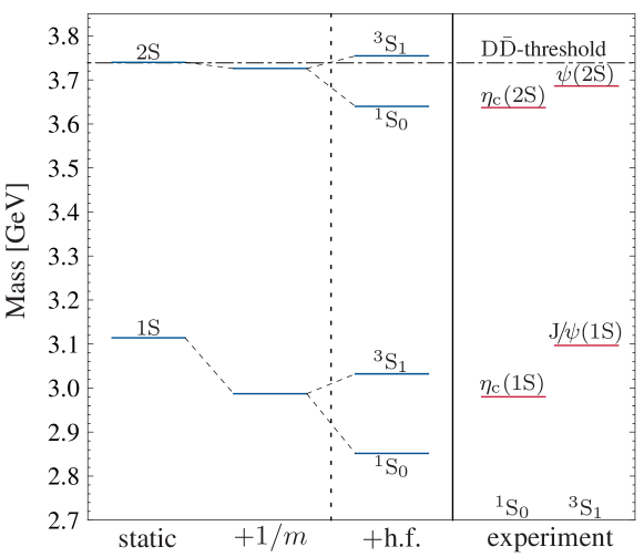
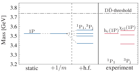
Figure 11: Charmonium spectrum in comparison with experiment. Static plus order $1/m$ results are shown on the left, with additional hyperfine effects (h.f.) added phenomenologically.

As expected, the influence of the $1/m$ term in the potential is much stronger for charmonium than for bottomonium (see Fig. 11). For charmonium we choose the potential-subtracted mass in Eq. (15) (reflecting the unknown constants in $V^{(0)}$ and $V^{(1)}$) such that the measured $\text{h}_{\text{c}}\text{(1P)}$ energy is reproduced without $1/m$ corrections. With this choice, however, the $V^{(1)}$ part produces a downward shift of $127$ MeV in the 1S states ($\eta_{\text{c}}$ and $\text{J}\!/\!\psi$) relative to the static result. This shift is too large in comparison with the measured $\eta_{\text{c}}$ and $\text{J}\!/\!\psi$ energies.

The 1S states are naturally more sensitive to $1/m$ corrections than 1P and 2S states because of the leading $1/r^{2}$ short-distance behavior of $V^{(1)}$. Hence the large shift of the 1S energy level at order $1/m$ does not come unexpectedly. It is nevertheless evident that, no matter which choice is adopted for adjusting the unknown constant in $V^{(1)}$, the 1S and 1P states of charmonium cannot be simultaneously reproduced at order $1/m$. Unlike the situation in bottomonium, corrections of order $1/m^{2}$ are presumably large in charmonium.

A manifestation of substantial $1/m^{2}$ effects is the relatively large observed splitting of $117$ MeV between $\eta_{\text{c}}$ and $\text{J}\!/\!\psi$, driven by an effective coupling strength ($\alpha_{s}^{\text{eff}}/m^{2}$ with $\alpha_{s}^{\text{eff}}=0.3$ in the phenomenological $\delta V_{\text{spin}}$ of Eq. (16)) that is an order of magnitude larger than for bottomonium. A systematic investigation of the $1/m^{2}$ potential, $V^{(2)}$ in Eq. (11), is mandatory now that lattice QCD data for $V^{(2)}$ are becoming available Koma:2006fw ; Koma:2010zz .

VI Charm and bottom quark masses:
potential-subtracted and $\overline{\text{MS}}$ schemes

The static potential is determined up to an overall constant. Introducing the potential-subtracted (PS) quark mass as

$$m_{\text{PS}}(\mu_{f})=m_{\text{pole}}+\frac{1}{2}\intop_{|\vec{q}\,|<\mu_{f}}\!\frac{d^{3}q}{(2\pi)^{3}}\,\tilde{V}^{(0)}(|\vec{q}\,|)=m_{\text{pole}}+\frac{1}{4\pi^{2}}\intop_{0}^{\mu_{f}}\!dq\,q^{2}\,\tilde{V}^{(0)}(q)$$ (18)

in terms of the pole mass of the charm or bottom quark, this $m_{\text{PS}}$ absorbs the unknown constant and does not suffer from the leading renormalon ambiguity Beneke:1998rk ; Hoang:1998nz . With the previous choice of the constant to reproduce the measured $\Upsilon\text{(2S)}$ energy, we find the value $m_{\text{PS}}(\mu_{f}\!=\!0.908\ \text{GeV})=4.78$ GeV in the PS mass scheme. In the charmonium case we fit to the $\text{h}_{\text{c}}(\text{1P})$ energy and find $m_{\text{PS}}(\mu_{f}\!=\!0.930\ \text{GeV})=1.39$ GeV. To convert the PS mass to the mass in the more commonly used $\overline{\text{MS}}$ scheme, it is necessary to introduce the pole mass $m_{\text{pole}}$ as an intermediate step. The relation between $m_{\text{pole}}$ and $m_{\text{PS}}$ reads Beneke:1998rk :

$$m_{\text{pole}}=m_{\text{PS}}(\mu_{f})+\frac{C_{F}\,\alpha_{s}(\mu)\,\mu_{f}}{\pi}\bigg{\{}1+\frac{\alpha_{s}(\mu)}{4\pi}\bigg{[}a_{1}-\beta_{0}\bigg{(}\!\ln\frac{\mu_{f}^{2}}{\mu^{2}}-2\bigg{)}\bigg{]}\\ +\bigg{(}\frac{\alpha_{s}(\mu)}{4\pi}\bigg{)}^{2}\bigg{[}a_{2}-(2a_{1}\beta_{0}\!+\!\beta_{1})\bigg{(}\!\ln\frac{\mu_{f}^{2}}{\mu^{2}}-2\bigg{)}+\beta_{0}^{2}\bigg{(}\!\ln^{2}\frac{\mu_{f}^{2}}{\mu^{2}}-4\ln\frac{\mu_{f}^{2}}{\mu^{2}}+8\bigg{)}\bigg{]}+\mathcal{O}(\alpha_{s}^{3})\bigg{\}}\,,$$ (19)

with the same conventions as in Section II. Note that a renormalization scale $\mu$ appears in the coupling. In the following $\mu$ is set equal to the $\overline{\text{MS}}$ mass $\overline{m}\equiv m_{\overline{\text{MS}}}(m_{\overline{\text{MS}}})$. This $\overline{m}$ is not known at that point and has to be computed iteratively. In a second step the pole mass is converted to the $\overline{\text{MS}}$ mass Chetyrkin:1999qi ; Melnikov:2000qh :

$$\frac{m_{\text{pole}}}{\overline{m}}=1 +\frac{4}{3}\bigg{(}\frac{\alpha_{s}(\overline{m})}{\pi}\bigg{)}+\bigg{(}\frac{\alpha_{s}(\overline{m})}{\pi}\bigg{)}^{2}(-1.0414\,n_{f}+13.4434)$$

$$+\bigg{(}\frac{\alpha_{s}(\overline{m})}{\pi}\bigg{)}^{3}(0.6527\,n_{f}^{2}-26.655\,n_{f}+190.595)+\mathcal{O}(\alpha_{s}^{4})\,.$$ (20)

Note that both relations (19) and (VI), taken individually, show a poorly convergent behavior whereas the relation between $m_{\text{PS}}(\mu_{f})$ and $\overline{m}$ is expected to be stable. This is in fact confirmed numerically. Using $\mu_{f}=0.908$ GeV (from Section III) one obtains the value $\overline{m}_{\text{b}}=4.27$ GeV for the bottom quark; with $\mu_{f}=0.930$ GeV one finds $\overline{m}_{\text{c}}=1.24$ GeV for the charm quark.

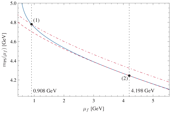
Figure 12: Scale dependence of $m_{\text{PS}}(\mu_{f})$ for the bottomonium case. The solid curve shows the numerical $\mu_{f}$ dependence from Eq. (18). The dashed and dashed-dotted curves show the $\mu_{f}$ dependence given by Eq. (19) at different matching points. Point (2) is preferred to point (1) for the determination of $\overline{m}_{\text{b}}$.

However, as shown in Fig. 12, the $\mu_{f}$ dependence of $m_{\text{PS}}(\mu_{f})$ (Eq. (19)) differs for $\mu_{f}\!\ll\!\overline{m}$ from the $\mu_{f}$ dependence coming from variations of the cutoff in the numerical integral (solid line). Instead of matching at $\mu_{f}=0.908$ GeV it is obviously preferable to use the numerical $\mu_{f}$ dependence first to translate $m_{\text{PS}}(\mu_{f})$ into $m_{\text{PS}}(\overline{m})$ and then apply Eqs. (19) and (VI) to translate this value into the $\overline{\text{MS}}$ scheme. By this method the extraction of $\overline{m}$ becomes independent of the value of $\mu_{f}$ used in the construction of the potential. This leads to improved mass values, $\overline{m}_{\text{b}}=4.20$ GeV for the bottom quark and $\overline{m}_{\text{c}}=1.23$ GeV for the charm quark in the $\overline{\text{MS}}$ scheme.

To determine values for the quark masses at order $1/m$ a redefinition of the PS mass is required:

$$m_{\widehat{\text{PS}}}(\mu_{f},\mu_{f}^{\prime})\equiv m_{\text{PS}}(\mu_{f})-\frac{1}{8m}C_{F}C_{A}\alpha_{s}^{2}(\overline{m})\,\mu_{f}^{\prime\,2}\,.$$ (21)

The $1/m$-term stems from an analogous calculation as in the static case. The renormalization scale $\mu$ that appears in the coupling has again been identified with $\overline{m}$. We determine $m_{\widehat{\text{PS}}}(\mu_{f},\mu_{f}^{\prime})$ for the b- and c-quark by fitting to the empirical $\Upsilon\text{(2S)}$ and $\text{h}_{\text{c}}(\text{1P})$ energies, respectively, and convert these values numerically to $m_{\widehat{\text{PS}}}(\overline{m},\overline{m})$. This leads in a second step to the $1/m$-improved $\overline{\text{MS}}$ values $\overline{m}_{\text{b}}=4.18$ GeV for the bottom quark and $\overline{m}_{\text{c}}=1.28$ GeV for the charm quark. In Table 1 the quark masses in the $\overline{\text{MS}}$ scheme found in our approach are summarized and compared to values given by the Particle Data Group Nakamura:2010zzi .

$\overline{\text{MS}}$ masses [GeV]
	Static	Static + $\mathcal{O}(1/m)$	PDG 2010
Bottom quark	$4.20\pm 0.04$	$4.18^{+0.05}_{-0.04}$	$4.19^{+0.18}_{-0.06}\vphantom{\Big{(}}$
Charm quark	$1.23\pm 0.04$	$1.28^{+0.07}_{-0.06}$	$1.27^{+0.07}_{-0.09}\vphantom{\Big{(}}$

Table 1: Comparison of quark masses obtained in our approach (leading order plus order $1/m$ corrections) with the values listed by the Particle Data Group (PDG) Nakamura:2010zzi . See text for details concerning error estimates.

We have performed error estimates for the quark masses, reflecting uncertainties in the potentials (static and order $1/m$). Additional uncertainties are included from our specific choice of matching to the empirical $\Upsilon\text{(2S)}$ and $\text{h}_{\text{c}}(\text{1P})$ energies. The errors at order $1/m$ have increased in comparison to those for the static case since they incorporate in addition the error band from $V^{(1)}$. The error estimates at order $1/m$ do not include possible further uncertainties appearing at order $1/m^{2}$.

VII Summary

Improved bottomonium and charmonium potentials have been derived up to and including order $1/m$ in the heavy quark masses by systematically matching perturbative QCD results to accurate lattice QCD data at an intermediate distance scale, $r=0.14$ fm. A single constant (the potential-subtracted quark mass) is adjusted to reproduce the $\Upsilon\text{(2S)}$ and $\text{h}_{\text{c}}(\text{1P})$ masses, respectively. The predicted pattern of all other subthreshold states agrees well with the empirical bottomonium spectroscopy. For charmonium, $1/m$ effects are far more pronounced, as expected. The potential-subtracted heavy quark masses at order $1/m$, when translated to $\overline{\text{MS}}$ masses, agree well with those listed by the Particle Data Group. In a next step, corrections of order $1/m^{2}$ will be studied along the same lines.

- (1) M. Beneke, Phys. Lett. B434, 115 (1998).
- (2) A. H. Hoang, M. C. Smith, T. Stelzer, and S. Willenbrock, Phys. Rev. D59, 114014 (1999).
- (3) M. Peter, Phys. Rev. Lett. 78, 602 (1997).
- (4) M. Peter, Nucl. Phys. B501, 471 (1997).
- (5) Y. Schröder, Phys. Lett. B447, 321 (1999).
- (6) N. Brambilla, A. Pineda, J. Soto, and A. Vairo, Phys. Rev. D60, 091502 (1999).
- (7) A. V. Smirnov, V. A. Smirnov, and M. Steinhauser, Phys. Rev. Lett. 104, 112002 (2010).
- (8) C. Anzai, Y. Kiyo, and Y. Sumino, Phys. Rev. Lett. 104, 112003 (2010).
- (9) B. A. Kniehl, A. A. Penin, V. A. Smirnov, and M. Steinhauser, Nucl. Phys. B635, 357 (2002).
- (10) T. van Ritbergen, J. A. M. Vermaseren, and S. A. Larin, Phys. Lett. B400, 379 (1997).
- (11) A. Pineda, J. Phys. G29, 371 (2003).
- (12) N. Brambilla, A. Vairo, X. Garcia i Tormo, and J. Soto, Phys. Rev. D80, 034016 (2009).
- (13) S. Bethke, Eur. Phys. J. C64, 689 (2009).
- (14) K. G. Chetyrkin, B. A. Kniehl, and M. Steinhauser, Phys. Rev. Lett. 79, 2184 (1997).
- (15) G. S. Bali et al., Phys. Rev. D62, 054503 (2000).
- (16) S. Necco and R. Sommer, Nucl. Phys. B622, 328 (2002).
- (17) N. Brambilla, X. Garcia i Tormo, J. Soto, and A. Vairo, Phys. Rev. Lett. 105, 212001 (2010).
- (18) N. Brambilla, A. Pineda, J. Soto, and A. Vairo, Phys. Rev. D63, 014023 (2000).
- (19) Y. Koma, M. Koma, and H. Wittig, Phys. Rev. Lett. 97, 122003 (2006).
- (20) M. Koma, Y. Koma, and H. Wittig, PoS Confinement8, 105 (2008).
- (21) G. Perez-Nadal and J. Soto, Phys. Rev. D79, 114002 (2009).
- (22) Y. Koma and M. Koma, Nucl. Phys. B769, 79 (2007).
- (23) Y. Koma and M. Koma, AIP Conf. Proc. 1322, 298 (2010).
- (24) K. G. Chetyrkin and M. Steinhauser, Phys. Rev. Lett. 83, 4001 (1999); Nucl. Phys. B 573, 617 (2000).
- (25) K. Melnikov and T. v. Ritbergen, Phys. Lett. B482, 99 (2000).
- (26) K. Nakamura et al. (Particle Data Group), J. Phys. G37, 075021 (2010).