High-Performance Algorithm for Calculating Non-Spurious Spin- and Parity-Dependent Nuclear Level Densities

Abstract

A new high-performance algorithm for calculating the spin- and parity-dependent shell model nuclear level densities using methods of statistical spectroscopy in the proton-neutron formalism was recently proposed. When used in valence spaces that cover more than one major harmonic oscillator shell, this algorithm mixes the genuine intrinsic states with spurious center-of-mass excitations. In this paper we present an advanced algorithm, based on the recently proposed statistical moments method, that eliminates the spurious states. Results for unnatural parity states of several $sd$-shell nuclei are presented and compared with those of exact shell model calculations and experimental data.

I Introduction

In this article we make a next step towards a reliable practical algorithm for calculating the level density in a finite many-body system with strong interaction between the constituents. Our primary object of applications is the atomic nucleus but the same techniques can be applied to other mesoscopic systems, such as atoms in traps heiselberg02 and quantum dots reimann02 . Being a key element in the description of nuclear reactions and quantum transport in general, the many-body level densities are also interesting from the fundamental viewpoint since, at not very high excitation energy, the growth of the level density reflects the interplay of interactions inside the system. The energy dependence of the level density may indicate the phase transformations smoothed out in finite systems: pairing quenching in nuclei big ; HZppt and small metallic particles leavens81 , or magnetic effects in small quantum dots gonzalez02 . The correct reproduction of the level density serves as the first step to recognizing the regular or chaotic nature of spectral statistics in nuclei brody81 ; big ; aberg09 , complex atoms grib and quantum dots ulloa97 .

The information on spin- and parity-dependent nuclear level densities (SPNLD) represents a critical ingredient for the theory of nuclear reactions, including those of astrophysical interest. For example, the routinely used Hauser-Feschbach approach HF requires the knowledge of nuclear level densities for certain quantum numbers $J^{\pi}$ of spin and parity in the window of excitation energy around the particle threshold rauscher97 ; moller09 . The nuclear technology requires the level density in the region of compound resonances close to the neutron separation energy. Therefore, a lot of effort has been invested in finding the accurate SPNLD, starting with the classical Fermi-gas approximations bethe36 ; cameron ; ericson and progressing to the sophisticated mean-field combinatorics gor-icomb-08 ; gor-fis-09 ; aberg09 and various shell model approaches with residual interactions in large valence spaces Eric97 ; Alhassid97 ; Langanke98 ; alhassid00 ; jtpden ; jdenrc ; alhassid07 ; alhassid09 ; SH2010 .

Earlier we developed a strategy jtpden ; jdenrc ; nic8den ; epl10 ; SH2010 of calculating the shell model SPNLD using methods of statistical spectroscopy wongbook ; kotabook . In the basic version of this approach, all basis states that can be built within a selected spherical single-particle valence space are taken into account. However, when the valence space spans more than one harmonic oscillator major shell, the shell model states include spurious excitations of the center-of-mass (CM). Apart from the level density problem, the correct separation of the spurious states is important for finding the physical response of the system to external fields, for example in the case of the excitation of isoscalar giant resonances. Over the years, shell model practitioners developed techniques lawson that allow one to push these unwanted states to energies higher than those of interest for low-energy phenomena. These techniques involve (i) separation of basis states in the so-called $N\hbar\omega$ subspaces that can exactly factorize in the CM-excited and intrinsic states, and (ii) the addition to the nuclear Hamiltonian of a CM-part multiplied by a properly chosen positive constant. Unfortunately, the second ingredient leads to a multimodal distribution of levels and it is not appropriate for the methods of statistical spectroscopy.

In a recent letter dencom , we proposed a shell-model algorithm for removing the spurious CM contributions from the SPNLD that works if one knows the SPNLD for each $N\hbar\omega$ subspace. These contributions are unimodal and can be described using methods of statistical spectroscopy, provided that one can calculate the necessary moments of the Hamiltonian in $N\hbar\omega$ subspaces. In the present paper we formulate and utilize a high-performance algorithm that can calculate the configuration centroids and the widths of the Hamiltonian in $N\hbar\omega$ subspaces. This algorithm will be used for calculating the non-spurious level density for unnatural parity states of several $sd$-shell nuclei. Comparison with the exact shell model results and/or experimental data will be also presented.

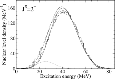
Figure 1: ²⁰Ne, $1\hbar\omega$, negative parity. Comparison of nuclear level densities from the exact shell model (stair lines) and from the moments method (straight lines). Dashed lines correspond to total densities with spurious states included; solid lines correspond to non-spurious densities without spurious states. Dotted lines present the spurious density.

II Spin- and Parity-dependent configuration moments method

We start closely following the approach proposed in Refs. jtpden ; jdenrc ; SH2010 . For reader’s convenience, we repeat first the main equations of the moments method. According to this approach, one can calculate the level density $\rho$ as a function of excitation energy $E$ in the following way:

$$\rho(E,\alpha)=\sum_{\kappa}D_{\alpha\kappa}\cdot G_{\alpha\kappa}(E),$$ (1)

where $\alpha=\{n,J,T_{z},\pi\}$ is a set of quantum numbers, the total number of particles, $n$, total spin, $J$, isospin projection, $T_{z}$, and parity, $\pi$; for the level density, in contrast to the state density, the spin degeneracy $2J+1$ is excluded. The sum over configurations $\kappa$ in Eq. (1) spans all possible (for the certain values of $n,T_{z}$, and $\pi$) ways of distributing $n$ particles over $q$ spherical single-particle orbitals. Each configuration $\kappa$ is presented by a set of occupation numbers $\kappa=\{n_{1},n_{2},...\;,n_{q}\},$ where $n_{j}$ is the number of particles occupying the spherical single-particle level $j$, $\sum_{j}n_{j}=n$.

The energy dependence of the density $\rho$ is expressed by finite-range Gaussian functions, $G_{\alpha\kappa}$, defined as in Ref. jtpden :

$$G_{\alpha\kappa}(E)=G(E+E_{{\rm g.s.}}-E_{\alpha\kappa},\sigma_{\alpha\kappa}),$$ (2)

$$G(x,\sigma)=C\cdot\left\{\begin{array}[]{ll}\mbox{exp}\left(-x^{2}/2\sigma^{2}\right)&,\;\;|x|\leq\eta\cdot\sigma\\ 0&,\;\;|x|>\eta\cdot\sigma\\ \end{array}\right.,$$ (5)

where the parameters $E_{\alpha\kappa}$ and $\sigma_{\alpha\kappa}$ will be defined later, $E_{{\rm g.s.}}$ is the ground state energy, $\eta$ is the cut-off parameter, and $C$ is the normalization factor corresponding to the condition $\int_{-\infty}^{+\infty}G(x,\sigma)dx=1$. Although $\eta$ can be treated as a free parameter, we know from the previous works (see for example SH2010 ; epl10 ; nic8den ) that its optimal value is $\eta\sim 3$, which allows us to get a finite-range distribution for the density and, practically, do not change each Gaussian contribution. Finally, the dimension $D_{\alpha\kappa}$ in Eq. (1) gives the correct normalization for each finite-range Gaussian being equal to the number of many-body states with given set of quantum numbers $\alpha$ that can be built for a given configuration $\kappa$.

The density distribution $\rho(E)$, especially its low-energy part, is very sensitive to the choice of the ground state energy $E_{gs}$. This origin of the energy scale is an external parameter for the moments method. To calculate it we need to use supplementary methods, such as the shell model.

The parameters $E_{\alpha\kappa}$ and $\sigma_{\alpha\kappa}$ in Eq. (2) are the fixed-$J$ configuration centroids and widths. They essentially present the average energy and the standard deviation for the set of many-body states with a given set of quantum numbers $\alpha$ within a given configuration $\kappa$. For a Hamiltonian containing one- and (antisymmetrized) two-body parts of interaction,

$$H=\sum_{i}\epsilon_{i}a^{\dagger}_{i}a_{i}+\frac{1}{4}\sum_{ijkl}V_{ijkl}a^{\dagger}_{i}a^{\dagger}_{j}a_{l}a_{k},$$ (6)

the fixed-$J$ centroids and widths can be expressed in terms of the traces of the first and second power of this Hamiltonian SH2010 , Tr$[H]$ and Tr$[H^{2}]$, for each configuration $\kappa$:

$$E_{\alpha\kappa}=\langle H\rangle_{\alpha\kappa},$$ (7)

$$\sigma_{\alpha\kappa}=\sqrt{\langle H^{2}\rangle_{\alpha\kappa}-\langle H\rangle^{2}_{\alpha\kappa}},$$ (8)

where

$$\langle H\rangle_{\alpha\kappa}=\mbox{Tr}^{(\alpha\kappa)}[H]/D_{\alpha\kappa},$$ (9)

$$\langle H^{2}\rangle_{\alpha\kappa}=\mbox{Tr}^{(\alpha\kappa)}[H^{2}]/D_{\alpha\kappa}.$$ (10)

Every trace, such as $\mbox{Tr}^{(\alpha\kappa)}[\cdots]$, contains the sum of all diagonal matrix elements, $\sum\langle\nu,J|\cdots|\nu,J\rangle$, over all many-body states $\left|\nu,J\right>$ within given configuration $\kappa$ and with certain set of quantum numbers $\alpha$.

As in our previous work SH2010 we derive these traces for the fixed total spin projection $J_{z}$, rather than for fixed $J$. Technically, it is much more easier to construct many-body states with a given total spin projection. The $J$-traces can be easily expressed through the $J_{z}$-traces using the standard relation

$$\mbox{Tr}^{(J)}[\cdots]=\mbox{Tr}^{(J_{z})}[\cdots]_{{}_{J_{z}=J}}-\mbox{Tr}^{(J_{z})}[\cdots]_{{}_{J_{z}=J+1}}.$$ (11)

In Eq. (11) we omitted all quantum numbers, except for the projection $J_{z}$ and the total spin $J$.

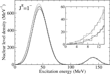
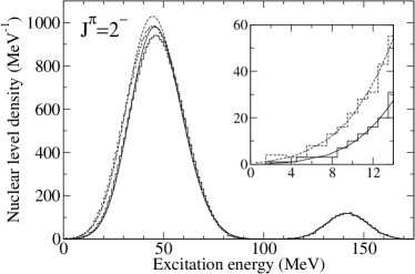
Figure 2: ²²Na, $1\hbar\omega$, negative parity. Comparison of nuclear level densities from the exact shell model (stair lines) and from the moments method (straight lines). Dashed lines correspond to total densities with spurious states included; solid lines correspond to non-spurious densities without spurious states. Right side of the figures presents the spurious density.

We will use the same label $\alpha$ to denote a set of quantum numbers that includes either the fixed $J_{z}$ or the fixed $J$, keeping in mind that Eq. (11) can always connect them. In every important case we will point out which set of quantum numbers was used. The expressions for the traces can be found in Ref. jaq79 , see also SH2010 and references there.

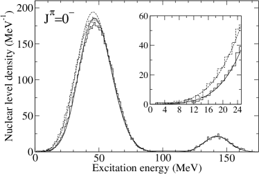
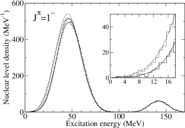
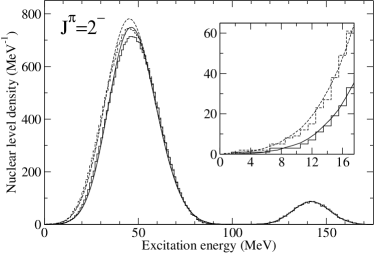
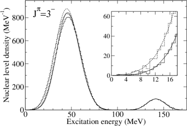
Figure 3: ²²Mg, negative parity. Comparison of nuclear level densities between exact shell model (stair lines) and moments method (straight lines). Dashed lines correspond to total densities with spurious states. Solid lines correspond to non-spurious densities without spurious states. Right side of the figures present spurious density.

III New features of the algorithm

To remove the center-of-mass spurious states from the level density we follow the approach suggested in dencom . This approach assumes the knowledge of the level density within a restricted basis, and one needs to calculate partial densities $\rho(E,\alpha,N)$ for a given number $N$ of excitations $\hbar\omega$, where the classification of states in terms of the harmonic oscillator $N\hbar\omega$ excitations is applied. It has to be mentioned that such a splitting is clearly an approximation since it refers to the harmonic oscillator potential and the level scheme. The harmonic oscillator frequency $\omega$, being an auxiliary parameter has no strict a-priori definition. Nevertheless, as we will demonstrate, the suggested method results are independent of $\hbar\omega$.

According to this method a pure (without admixture of spurious states) level density $\rho^{(0)}(E,J,N)$ can be expressed through the total (all states included) level density $\rho(E,J,N)$ for the same values of arguments and through the pure densities of lower $N$, Ref. dencom :

$$\rho^{(0)}(E,J,N)=\rho(E,J,N)-$$

$$-\sum_{K=1}^{N}\sum_{J_{K}=J_{{\rm min}}}^{N,{\rm step}\;2}\sum_{J^{\prime}=|J-J_{K}|}^{J+J_{K}}\rho^{(0)}(E,J^{\prime},(N-K)).$$ (12)

Here, for simplicity, we omitted all quantum numbers indicatting only total spin $J$ representing the set $\alpha$. In order to make these recursive equations complete we need a boundary condition that can be obtained from the $0\hbar\omega$ case which is free of spurious admixtures,

$$\rho^{(0)}(E,J,0)=\rho(E,J,0).$$ (13)

For example, if we are interested in the $1\hbar\omega$ level density, we come to the following relation:

$$\rho^{(0)}(E,J,1)=\rho(E,J,1)-\sum_{J^{\prime}=|J-1|}^{J+1}\rho(E,J^{\prime},0).$$ (14)

To calculate these partial level densities with the restricted values of excitation numbers $N$ we need to slightly change the previous algorithm. By construction, each configuration $\kappa$ in Eq. (1) has a certain excitation number $N_{\kappa}$ that can be defined as

$$N_{\kappa}=\sum_{a=1}^{n}\nu_{a}-N_{0},$$ (15)

where the sum runs over all $n$ nucleons, $\nu_{a}$ is the excitation number of the single-particle level occupied by the nucleon $a$, and, for our convenience, we shift the result by the lowest value of the sum, $N_{0}$, so that $N_{\kappa}$ starts with zero: $N_{\kappa}=0,1,2,\cdots$. Knowing $N_{\kappa}$ we can restrict the sum in Eq. (1) by including only those configurations $\kappa$ which correspond to the desirable values of excitation numbers.

For each configuration $\kappa$ we need to calculate the $J$-fixed width and centroid, $\sigma_{\alpha\kappa}$, $E_{\alpha\kappa}$, defined by Eqs. (7) and (8). There is no problem with the centroid calculation, $E_{\alpha\kappa}\sim\mbox{Tr}^{(\alpha\kappa)}[H]$, since it remains  unchanged, we just need to select the configurations $\kappa$ of our interest. The width calculation requires more attention. The problem is that the widths depend on the trace of the second power of the Hamiltonian, $\mbox{Tr}^{(\alpha\kappa)}[H^{2}]$, and if we want to restrict the basis we have to take care of the intermediate states $-$ they also have to be restricted,

$$\mbox{Tr}^{(\alpha\kappa)}[H^{2}]=\sum_{\lambda\in\kappa}\sum_{\mu(N_{\mu}\in R)}\langle\lambda|H|\mu\rangle\langle\mu|H|\lambda\rangle.$$ (16)

Here the sum over $\lambda$ includes all many-body states within the given configuration $\kappa$ and with certain set of quantum numbers $\alpha$. In contrast to this, the sum over $\mu$ includes all possible intermediate states regardless to configurations and quantum numbers, but only restricted by the desirable excitation numbers $N$. In Eq. (16), $R$ represents the set of all such many-body states defined by the allowed $N$. In our previous algorithm, we could remove the intermediate sum using the completeness relation, $\sum_{\mu}\left|\mu\right>\left<\mu\right|=1$, and express the width in terms of the traces over single-particle excitations ($D-$structures, as in Eq. (11) of Ref. SH2010 ). Now that is impossible, and we need to treat the situation differently.

One possible way to proceed here is still to follow the approach suggested in Ref. jdenrc , where the “restricted” $D-$structures were introduced, see Eqs. (11,12) in this reference. Here we propose an alternative solution, which may be easier to implement as an efficient computer algorithm. The single-particle part of the Hamiltonian (6) does not create any problems. Indeed the one-body operators of the $a^{\dagger}_{i}a_{i}$ type do not change the excitation number $N$, so that all states $|\mu\rangle$ in Eq. (16) have the same $N_{\mu}$ as the states $|\lambda\rangle$ all of which have the same excitation number defined by the configuration $\kappa$, $N_{\lambda}=N_{\kappa}$. The two-body part of the Hamiltonian has the matrix elements

$$\langle\mu|V|\lambda\rangle=\,\frac{1}{4}\,\sum_{ijkl}V_{ijkl}\langle\mu|a^{\dagger}_{i}a^{\dagger}_{j}a_{l}a_{k}|\lambda\rangle$$ (17)

which indeed can mix the states with different excitation numbers. Each member of the sum in Eq. (17) produces a certain change of the number of excitation quanta, $\Delta N_{ijkl}$,

$$\Delta N_{ijkl}=\nu_{i}+\nu_{j}-\nu_{k}-\nu_{l},$$ (18)

where $\nu_{i}$ is the excitation number of the single-particle level $i$. It is important that $\Delta N_{ijkl}$ reflects the internal property of the interaction operator $a^{\dagger}_{i}a^{\dagger}_{j}a_{l}a_{k}$ and does not depend on the many-body states. To deal with the sum over $\mu$ in Eq. (16), we notice that $N_{\mu}=N_{\lambda}+\Delta N_{ijkl}$, and therefore the restriction on $N_{\mu}$ can be reformulated in terms of the equivalent restriction on the single-particle levels,

$$\sum_{\mu(N_{\mu}\in R)}\;\sum_{ijkl}\,\equiv\sum_{\mu}\left[\sum_{ijkl}\right]_{R_{\Delta}},$$ (19)

where $R_{\Delta}$ means that the sum inside the parentheses is restricted by $N_{\lambda}+\Delta N_{ijkl}\in R$.

In order to satisfy the condition of Eq. (17) we just need to keep those sets of the single-particle levels $i,j,l,$ and $k$ in (17) for which the excitation quanta of the $|\lambda\rangle$ state plus the shift $\Delta N$, caused by the corresponding operator $a^{\dagger}_{i}a^{\dagger}_{j}a_{l}a_{k}$, satisfy this restriction condition. For example, if we want to take into account only $0\hbar\omega$ and $2\hbar\omega$ classes of states, and the $|\lambda\rangle$ states belong to the, let’s say, $0\hbar\omega$ class, then the allowed shifts of excitation quantum numbers will be $\Delta N=0,2$. All other terms in Eq. (17) must be ignored. Thus, we can use the old expressions for the $D$-structures without changes (see Eq. (12) of Ref. SH2010 ), which is an essential advantage, but it is necessary to enforce the appropriate restrictions on the sums over single-particle quantum numbers.

The final result can be written as

$$\mbox{Tr}^{(\alpha\kappa)}[H^{2}]=$$

$$=\sum_{i}\epsilon^{2}_{i}D^{[i]}_{\alpha\kappa}+\sum_{i<j}\left[2\epsilon_{i}\epsilon_{j}+2(\epsilon_{i}+\epsilon_{j})V_{ijij}\right]D^{[ij]}_{\alpha\kappa}$$

$$+\sum_{(i<j)\neq l}2\epsilon_{l}V_{ijij}D^{[ijl]}_{\alpha\kappa}+\sum_{(i<j)\neq(q<l)}V_{ijij}V_{qlql}D^{[ijql]}_{\alpha\kappa}$$

$$+\left[\sum_{i<j,\;q<l}V^{2}_{ijql}D^{[ql]}_{\alpha\kappa}+\sum_{(i<j)\neq(q<l)}V^{2}_{ijql}D^{[ijql]}_{\alpha\kappa}\right.$$

$$\left.-\sum_{i,\;(q<l)\neq j}V^{2}_{ijql}D^{[jql]}_{\alpha\kappa}\right]_{R_{1}}$$

$$+\left[\sum_{l,\;(i<j)\neq q}2V_{liiq}V_{ljjq}\left(D^{[ijq]}_{\alpha\kappa}-D^{[ijql]}_{\alpha\kappa}\right)\right]_{R_{2}},$$ (20)

where $R_{1}$ means that the sums inside the associated square bracket are restricted by $\left(N_{\kappa}+\nu_{i}+\nu_{j}-\nu_{q}-\nu_{l}\right)\in R$, and $R_{2}$ means that the sums in corresponding square bracket are restricted by $\left(N_{\kappa}+\nu_{l}-\nu_{q}\right)\in R$. The trace $D^{[i]}_{\alpha\kappa}=\mbox{Tr}^{(\alpha\kappa)}[a^{\dagger}_{i}a_{i}]$ can be interpreted as a number of many-body states with fixed projection $J_{z}$ (if we consider $J_{z}$-traces) and the single-particle state $i$ occupied, which can be constructed for the configuration $\kappa$; the notations for more complex traces are $D^{[ij]}_{\alpha\kappa}=\mbox{Tr}^{(\alpha\kappa)}[a^{\dagger}_{i}a^{\dagger}_{j}a_{j}a_{i}]$, $D^{[ijq]}_{\alpha\kappa}=\mbox{Tr}^{(\alpha\kappa)}[a^{\dagger}_{i}a^{\dagger}_{j}a^{\dagger}_{q}a_{q}a_{j}a_{i}]$, and so on. These $D$-structures were called propagation functions in Refs. SH2010 ; jaq79 . The detailed procedure for calculating these functions can be found in Ref. SH2010 .

In some applications, the restriction of the level density to one class of excitations described by the excitation number $N$, Eq. (10), might not be sufficient. For example, one could be interested in considering the class of $(0+2)\hbar\omega$ excitations. In those cases we select the maximum value $N_{{\rm max}}$ of allowed excitations, and all the states, including intermediate ones, are restricted according to

$$N\leq N_{{\rm max}}.$$ (21)

Such a restriction allows us to fully take into account the interference between the states of different $N\hbar\omega$ in Eq. (14). For example, if $N_{\rm max}=2$, there are two possible classes of states, $0\hbar\omega$ and $2\hbar\omega$, contributing to the width ($1\hbar\omega$ does not contribute because of opposite parity). The cross terms in Eq. (14), which are proportional to $|\langle 2\hbar\omega|H|0\hbar\omega\rangle|^{2}$, are equally important along with the diagonal contributions $|\langle 2\hbar\omega|H|2\hbar\omega\rangle|^{2}$ and $|\langle 0\hbar\omega|H|0\hbar\omega\rangle|^{2}$. If one is interested in the density of unnatural parity states, one could consider only the $1\hbar\omega$ excitations. In these cases there are no cross terms, since the $0\hbar\omega$ states have opposite parity, thus one can directly use Eqs. (10) and (12). Finally, one should mention that the present algorithm was integrated in our highly scalable moments code that was described in Ref. SH2010 .

IV Results

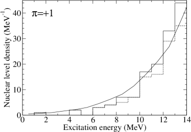
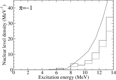
Figure 4: ²⁸Si, all $J$, both parities. Comparison of nuclear level densities from experiment (stair lines) and from the moments method calculation (straight line).

As a first example we consider ²⁰Ne in the $s-p-sd-pf$-shell model space. For this space we use the Warburton-Brown (WBT) interaction wbt . All calculations were done for $1\hbar\omega$ subspace and for negative parity. Fig. 1 presents the comparison of the exact shell model level densities (stair-dashed and stair-solid lines) with the densities calculated using the moments methods (straight-dashed and straight-solid lines). The all dashed lines present the total densities including spurious states. The solid lines present the pure non-spurious densities. For the shell model calculations the spurious states were removed with the help of the Lawson method lawson that adds to the actual Hamiltonian a shifted center-of-mass Hamiltonian, $H_{CM}$, multiplied by a constant $\beta$,

$$H\rightarrow H^{\prime}=H+\beta\left[\left(H_{CM}-\frac{3}{2}\hbar\omega\right)\frac{A}{\hbar\omega}\right].$$ (22)

The additional term pushes the all spurious states up and leaves the non-spurious density at low-lying excitation energy. In our calculations we used $\beta=5$. However, as it was mentioned in the introduction, the Lawson recipe can not filter spurious states for the moments method. To get the straight-solid lines on Fig. 1 we use the recursive method introduced in Eqs. (10-12). Finally, the dotted lines present the spurious densities itself calculated according to the second part of the right-hand side of Eqs. (10,12). To calculate the level density with the moments method we need to know the ground state energy and the cut-off parameter $\eta$. For ²⁰Ne, the ground state energy $E_{{\rm g.s.}}(^{20}\mbox{Ne})=-184.2$ MeV was calculated with the help of the shell model, WBT interaction, $0\hbar\omega$ subspace, and $\eta=2.8$.

Figs. 2 and 3 present similar results for ²²Na, ²²Mg, in the $s-p-sd-pf$ model space. The calculations also were done with the WBT interaction, for $1\hbar\omega$ subspace and negative parity. Stair lines refer to the shell model calculations, while straight lines present the results of the moments method. The only difference from Fig. 1 is the position of spurious states. The position of the spurious contribution to the total level density calculated with the shell model is naturally defined by the Lawson term and by parameter $\beta$. As we can see from the Figures, $\beta=5$ is shifting all spurious states to the region of excitation energies of order of 140 MeV. The spurious states calculated with the moments method are mostly located near the ground state energy. To compare the shape of the spurious part of the level density, we artificially shifted the results of the moments method by energy $\beta A$ MeV, which is 110 MeV for $A=22$ and $\beta=5$; after this, as seen from the Figures, the spurious states calculated with the shell model and Lawson term almost completely coincide with those calculated with the moments method and shifted afterwards. For all these cases we chose $\eta=2.8$ and ground state energies $E_{{\rm g.s.}}=-201.2$ MeV for ²²Na and $E_{{\rm g.s.}}=-202.3$ MeV for ²²Mg.

Figures 4 and 5 present bigger cases of ²⁶Al and ²⁸Si in the $s-p-sd-pf$ model space, for both positive and negative parities. The dimensions are very large, and it is not practical to get the level densities with the shell model. Only the ground state energies can be calculated for these cases in $0\hbar\omega$ subspace. With the WBT interaction, we got $E_{{\rm g.s.}}=-250.3$ MeV for ²⁶Al and $E_{{\rm g.s.}}=-285.0$ MeV for ²⁸Si. Figures 4 and 5 show comparisons of the level density calculated with the moments method, that is presented by straight lines, with experimental level densities presented by stair lines. There are two stair-like lines on each figure: the solid stair lines present an “optimistic” approach, when all experimental levels with uncertain parity were counted; oppositely, the dashed stair lines present a “pessimistic” approach, when only experimental levels with defined parity were counted.

It is needed to be mentioned that the real level densities must be greater than those presented by the stair-like lines since it is possible that many levels were missed in experiment. In spite of the fact that the WBT interaction was not really tested in such big model spaces (it was specifically designed for $A<20$), the agreement between the calculations using the moments method and experimental data is quite remarkable.

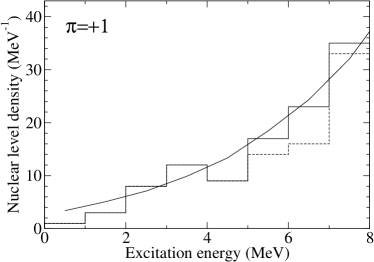
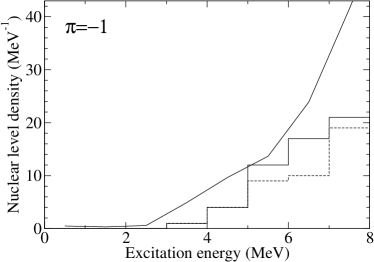
Figure 5: ²⁶Al, all $J$, both parities. Comparison of nuclear level densities from experiment (stair lines) and from the moments method calculation (straight line).

V Conclusions and Outlook

In conclusion, we developed a new high-performance algorithm to calculate the configuration centroids and widths of the nuclear Hamiltonian in $N\hbar\omega$ subspaces built in a valence space. These first two moments can be used to calculate the SPNLD in the associated $N\hbar\omega$ subspaces, which can be further mixed according to a recently proposed algorithm dencom for extracting the non-spurious SPNLD. This strategy can be used to calculate the non-spurious shell-model level density for unnatural parity, a long-standing problem in nuclear structure.

We tested our techniques by calculating the negative parity level density for several even-even $sd$-nuclei, where the exact $1\hbar\omega$ shell model diagonalization can be done and compared with the results of the newly proposed algorithm. In all cases the SPNLD results of our moments method describe very well the results of the full shell model calculations. We also compared the results of our moments method with the available experimental data for ²⁶Al and ²⁸Si. For the states of positive parity, the effective interaction is well suited and our level density compares successfully with the experimental data. For the negative parity states, there is no well-adjusted $1\hbar\omega$ effective interaction for the middle of the $sd$-shell. Using the WBT interaction that was tested up to about mass 20 wbt we obtain a reasonable description of the experimental data.

Certainly, there is a need of refined effective interactions for the unnatural parity states for the $sd$ nuclei, and our techniques could help improving their quality. The algorithm suggested in this article can be used to reliably predict for the first time the SPNLD for a large number of unstable nuclei relevant for the $rp$-process. The next steps could be directed to the more complicated cases, where the $N\hbar\omega$ space is incomplete. This will allow us to reformulate the approach for the realistic mean-field potentials when it will be possible to exclude the standard reference to harmonic oscillator and open the broad field of problems related to the cross sections and reaction rates. In parallel, the deep question should be addressed of the influence of continuum effects celardo11 on the density of levels which are in fact resonance quasistationary states.

VI Acknowledgemnets

R.S. and M.H. would like to acknowledge the DOE UNEDF grant No. DE-FC02-09ER41584 for support. M.H. and V.Z. acknowledge support from the NSF grant No. PHY-0758099.

References

- (1) H. Heiselberg and B. Mottelson, Phys. Rev. Lett. 88, 190401 (2002).
- (2) S.M. Reimann and M. Manninen, Rev. Mod. Phys. 74, 1283 (2002).
- (3) V. Zelevinsky, B.A. Brown, N. Frazier, and M. Horoi, Phys. Rep. 276, 85 (1996).
- (4) M. Horoi and V. Zelevinsky, Phys. Rev. C 75, 054303 (2007).
- (5) C.R. Leavens and E.W. Fenton, Phys. Rev. B 24, 5086 (1981).
- (6) A. Gonzalez and R. Capote, Phys. Rev. B 66, 113311 (2002).
- (7) T.A. Brody, J. Flores, J.B. French, P.A. Mello, A. Pandey, and S.S.M. Wong, Rev. Mod. Phys. 53, 385 (1981).
- (8) H. Uhrenholt, S. Åberg, P. Möller, and T. Ichikawa, arXiv:0901.1087.
- (9) V.V. Flambaum, A.A. Gribakina, G.F. Gribakin, and M.G. Kozlov, Phys. Rev. A 50, 267 (1994).
- (10) S.E. Ulloa and D. Prannkuche, Superlattices and Microstructures 21, 21 (1997).
- (11) W. Hauser and H. Feshbach, Phys. Rev. 87, 366 (1952).
- (12) T. Rauscher, F.-K. Thielemann, and K.-L. Kratz, Phys. Rev. C 56, 1613 (1997).
- (13) P. Möller et. al., Phys. Rev. C 79, 064304 (2009).
- (14) H. A. Bethe, Phys. Rev. 50, 332 (1936).
-
(15)
A.G.W. Cameron, Can. J. Phys. 36, 1040 (1958);
A. Gilbert and A. G. W. Cameron, Can. J. Phys. 43, 1446 (1965). -
(16)
T. Ericson, Nucl. Phys. 8, 265 (1958);
T. Ericson, Adv. in Phys. 9, 425 (1960). - (17) S. Goriely, S. Hilaire, and A. J. Koning, Phys. Rev. C 78, 064307 (2008).
- (18) S. Goriely, S. Hilaire, A. J. Koning, M. Sin, and R. Capote, Phys. Rev. C 79, 024612 (2009).
- (19) R.A. Sen’kov and M. Horoi, Phys. Rev. C 82, 024304 (2010).
- (20) W. E. Ormand, Phys. Rev. C 56, R1678 (1997).
- (21) H. Nakada and Y. Alhassid, Phys. Rev. Lett. 79, 2939 (1997).
- (22) K. Langanke, Phys. Lett. B 438, 235 (1998).
- (23) Y. Alhassid, G. F. Bertsch, S. Liu, and H. Nakada, Phys. Rev. Lett. 84, 4313 (2000).
- (24) Y. Alhassid, S. Liu, and H. Nakada, Phys. Rev. Lett. 99, 162504 (2007).
- (25) Y. Alhassid, L. Fang, and H. Nakada, Phys. Rev. Lett. 101, 082501 (2008).
- (26) M. Horoi, J. Kaiser, and V. Zelevinsky, Phys. Rev. C 67, 054309 (2003).
- (27) M. Horoi, M. Ghita, and V. Zelevinsky, Phys. Rev. C 69, 041307(R) (2004).
- (28) M. Scott and M. Horoi, EPL. 91, 52001 (2010).
- (29) M. Horoi, M. Ghita, and V. Zelevinsky, Nucl. Phys. A785, 142c (2005).
- (30) S. S. M. Wong, Nuclear Statistical Spectroscopy (Oxford University Press, 1986).
- (31) V.K.B. Kota and R.U. Haq, eds., Spectral Distributions in Nuclei and Statistical Spectroscopy (World Scientific, Singapore, 2010).
- (32) D.H. Gloeckner and H.R. Lawson, Phys. Lett. B 53, 313 (1974); see also F. Palumbo, Nucl. Phys. A99, 100 (1967).
- (33) M. Horoi and V. Zelevinsky, Phys. Rev. Lett. 98, 262503 (2007).
-
(34)
C. Jacquemin and S. Spitz, J. Phys. G 5, 195 (1979);
C. Jacquemin, Z. Phys. A 303, 135 (1981). - (35) E. K. Warburton and B. A. Brown, Phys. Rev. C 46, 923 (1992).
- (36) G.L. Celardo, N. Auerbach, F.M. Izrailev and V.G. Zelevinsky, Phys. Rev. Lett. 106, 042501 (2011).