Can persistent Epstein-Barr virus infection induce Chronic Fatigue Syndrome as a Pavlov reflex of the immune response?

Abstract

Chronic Fatigue Syndrome is a protracted illness condition (lasting even years) appearing with strong flu symptoms and systemic defiances by the immune system.
Here, by means of statistical mechanics techniques, we study the most widely accepted picture for its genesis, namely a persistent acute mononucleosis infection, and we show how such infection may drive the immune system toward an out-of-equilibrium metastable state displaying chronic activation of both humoral and cellular responses (a state of full inflammation without a direct ”causes-effect” reason).
By exploiting a bridge with a neural scenario, we mirror killer lymphocytes $T_{K}$ and $B$ cells to neurons and helper lymphocytes $T_{H_{1}},T_{H_{2}}$ to synapses, hence showing that the immune system may experience the Pavlov conditional reflex phenomenon: if the exposition to a stimulus (EBV antigens) lasts for too long, strong internal correlations among $B,T_{K},T_{H}$ may develop ultimately resulting in a persistent activation even though the stimulus itself is removed. These outcomes are corroborated by several experimental findings.

1 Introduction

Chronic Fatigue Syndrome (CFS) refers to a clinical condition characterized by a persistent debilitating fatigue, neurological problems and a combination of flu-like symptoms (e.g. headache, tender lymph nodes), ranging from at least $6$ months up to several years [1, 2, 3, 4, 5, 6].
The estimated worldwide prevalence of CFS is $0.4\%-1\%$ (meaning over $800000$ people in the United States and approximately $240000$ in the UK) with a striking socio-economical impact: The average annual total value of lost productivity in the United States is $\$9.1$ billion [7]. Such numbers propel a continued research to determine the cause and potential therapies for CFS, whose diagnosis is still symptom-based and whose origin remains elusive.

The resemblance of the CFS to a chronic form of acute infectious mononucleosis (AIM) has provoked investigation on whether this illness (whose etiologic agent is the Epstein-Barr virus, EBV), can prompt a chronic immune reaction in the body.

In this work we try to deepen this point: By bridging between a neural system and an adaptive immune system, we show that an associative learning phenomenon might underlie a transition from an AIM to a CFS state. Our model focuses on the mutual interaction and regulation between B and T lymphocytes: when stimulated by a viral load (e.g. EBV antigens), they get activated (AIM phase); the active phase is then supposed to relax to a quiescent state once the viral load ceases. Actually, we evidence that, during such a relaxing stage, the collective behavior of the components of the system can yield non-trivial phenomena: if AIM phase takes a relatively long time to recover (with respect to the timescale that sets the standard immune response, say two weeks), which is in turn related to the success of the EBV to elude immuno-surveillance, a strong correlation between the activation of B and T lymphocytes can be accomplished. As a result, when the viral load has vanished and B cells remain activate for their memory role, T cells can also maintain high concentration levels since they have “learnt” that active B cells are associated to infection. Therefore, as T cells display strong inflammatory properties, we may get a state of chronically active immune response (with CFS symptoms) despite the original infection is no longer in course.

We stress that our approach, by applying basic concepts of statistical mechanics to immunology, points out emerging possible mechanisms leading to the development of the CFS. Accordingly, we overlook the details of the interactions at work in order to focus on the very key mechanisms underlying the phenomena : Interestingly, as we will show, for this learning process to be properly fulfilled, T cells need to bypass the helper signal from specialized lymphocytes and this has been recently evidenced experimentally.

The paper is structured as follows: In Sec.$2$ we provide a basic background about EBV, CFS and associative learning; these topics will be merged in Sec. $3$, where we present our model. Then, in Sec. $4$, we show our analysis and results. Finally, our conclusions and discussions are in Sec. $5$, while all the mathematics involved is reported in the appendix.

2 Minimal background

In this section we provide a basic background about the main features concerning chronic fatigue syndrome, Epstein-Barr virus and classical conditioning, then, in the following sections we will merge such concepts to get an interpretation for the emergence and establishment of the CFS.

Before proceeding, it is worth introducing the main agents of the adaptive immune system [8], highlighting the details crucial for our framework.

2.1 The (adaptive) immune system

An immune response is generally triggered by the introduction into the body of an antigen, which may have either exogenous or endogenous origin (e.g. toxins, bacteria, viruses, cancerogenic cells). For instance, the genes of viruses that have infected a host cell can encode several proteins working as antigens.

B lymphocytes are the agents of the humoral (i.e. mediated by secreted antibodies) immune response. B-cells can produce antibodies upon their full activation, and are divided in clones (ensembles of cells all producing the same antibody). Activation requires antigen recognition as well as a signal from (antigen stimulated) $T_{H}$ cells. From activated B cells, specific for a given antigen, memory cells are eventually formed; these are long-life cells able to respond quickly to a following exposure to the same antigen.

Furthermore, Jerne, in the 70 s, suggested that antibodies must not only detect antigens, but also function as individual internal images of certain antigens and are themselves detected and acted upon. Via this mechanism, an effective network of interacting antibodies is formed, where network interactions provide a ”dynamical memory” of the immune system, by keeping the concentrations of antibodies at appropriate levels. This can be understood as follows: At a given time a virus is introduced in the body and starts replication. As a result, at high enough concentration, it is found by the proper B-lymphocyte counterpart. Let us consider, for simplicity, a virus as a string of information (i.e. $V=1001001$); the complementary B-cell producing the antibody Ig1, which can be thought of as the string $V^{*}=0110110$, will then start a clonal expansion and will release high levels of Ig1. Consequently, after a while, another B-cell will meet Ig1 and, as this antibody never (macroscopically) existed before, it will attack it by releasing the proper immunoglobulin Ig2 (i.e., the string $V^{**}=1001001$). The latter is actually a ”copy” (internal image) of the original virus but with no DNA or RNA charge inside.

T lymphocytes are the agents of cellular-mediated (i.e. not involving antibodies but directly cellular mechanisms such as lysis) response. As in standard literature, we focus on T-helper cells ($T_{H}$) and on T-cytotoxic or killer cells ($T_{K}$) which, when in their quiescent state, are referred to as T-CD8+ and T-CD4+, respectively. Quiescent T-cells can be activated upon contact with cells which have previously interacted with the antigen: T-killer cells can interact with the so-called Class I Major Histocompatibility Complex (MHC-I) expressed by all cells, while T-helper cells can interact with the so-called Class II Major Histocompatibility Complex (MHC-II) expressed only by antigen presenting cells (APC, e.g. macrophages, dendritic cells, B-cells). Active $T_{K}$ expresses killer functions destroying infected cells, while active $T_{H}$ assists other white blood cells in immunologic processes, including maturation of B cells and activation of cytotoxic T cells.

Every immune system cell is equipped to synthesize and release a variety of small molecules, called cytokines, that travel to other cells (both immune and not-immune) and up/down-regulate their growth; cytokines include interferons (IFNs) and interleukins (ILs).

Before turning to our framework, built of by means of statistical-mechanics techniques, we stress that several other aspects and techniques stemmed from the fields of mathematics and theoretical physics are becoming available to investigate the biological world, ranging from kinetic theories [11], to associative neural networks [12], to cellular automata and more [13, 14].

2.2 Chronic Fatigue Syndrome

The literature on CFS is very broad with hundreds of analysis carried out and a rich collection of data, yet the clinical implications of such findings remain uncertain and a unifying, globally accepted, picture of its etiology and pathophysiology is still missing [2, 3, 4, 5, 6].

Current theories are looking at the possibilities of neuroendocrine dysfunction, virus geneses, environmental toxins, genetic predisposition, or a combination of these: Several researches suggest that Epstein-Barr Virus (EBV), by prompting a chronic immune reaction in the body, might cause CFS. Indeed, the phenomenology reported is consistent with the idea that the syndrome may follow the occurrence of an infection yielding a massive immune response, which, for causes not yet completely clarified, may persist for long time, although the underlying infection is no longer in course. In fact, a CFS state is usually associated to an abnormal concentration and/or functioning of B-cells, T-cells and cytokines. Another interesting and robust immunological fact found in patients with CFS is an unusually high (more than $67\%$) increase of activated CD8+ cytotoxic T lymphocytes with MHC-II activation markers [15, 16, 17, 18, 19]. This will be a key point of our speculation.

From a symptomatology viewpoint, fatigue is a common symptom, but CFS is a multi-systemic disease including even post-exertional malaise, unrefreshing sleep, widespread muscle, joint pain, cognitive difficulties, chronic (often severe) mental and physical exhaustion, muscle weakness, hypersensitivity, orthostatic intolerance, digestive disturbances and more.

2.3 The Epstein-Bar virus

EBV is one of the most successful viruses, infecting over $90\%$ of humans and persisting for the lifetime of the person in a non pathogenic way [20, 21]. The infection can follow different pathways, in particular, it can turn in AIM (in up to $25\%$ cases [22]) or it can simply introduce the virus in the host organism in a non apparent way.

The virus aims to enter B-cells and, if successful, two outcomes are possible: In the first case the EBV begins a viral replication cycle (so called ”lytic phase”, a common feature of most viral infections), which induces the death of the infected cell, followed by the complete release of new virus particles, which are going to infect other cells; in the second case a state of latency (latent phase) is established where the “disguised” virus multiplies and stands by inside the cell, while no extracellular phenomena are observed, in such a way that no tackling by the immune system is evidenced.

During the primary infection, the latent cycle and the lytic cycle proceed in parallel and the immune system addresses most of its resources to the lytic cycle of viral replication; the infection can be asymptomatic, have non-specific symptoms, or be so massive to result in AIM. The acute phase can last up to several months and it ceases when the lytic cycle is interrupted by the immune responses or by the virus itself, then, the infection becomes latent and the host becomes a Healthy Carrier.

The possible persistence of the acute phase, despite a potent immune response against it, indicates that the virus has evolved strategies to elude the immune system. Among the different hypothesis, one has received particular attention [23]: the antigen BCRF1 can simulate the signal produced by IL-10 cytokines (which normally prompts leukocytes specialized against small-sized threatening agents, like EBV’s antigens) and determine a delay in the immune response. More precisely, the signal from BCRF1 inhibits the production of real IL-10; the lack of IL-10 polarizes the cellular immune response in the activation of a different kind of leukocyte, specialized in fighting against bigger-sized pathogens.

We finally report an interesting study [24] on T-cell responses, in the cases of a relatively brief (2-3 weeks) and of a protracted (4 months) acute phase. Although expansions of antigen-specific T-cells were observed in both situations, the T-cells reactivity occurred to be broad (i.e. addressed to several, both lytic and latent, antigens) and narrowly focused (i.e. mainly addressed to a singular antigen, the Early BMLF1), respectively.

Summarizing, a significant presence of antigen BCRF1 can determine a delay in the immune response. As a result, the immune activity may take a long time for the clearance of the infection; during this time the concentration of $T_{K}$ cells remains high and polarizes against BMLF1 antigen as if an internal self-reinforcement has occurred.

2.4 Statistical Mechanics of Pavlov effect

Classical conditioning, experimentally demonstrated by Pavlov [25], is probably the most famous form of associative learning. The typical procedure for inducing classical conditioning on a subject (e.g. a dog) involves presentation of a neutral stimulus (e.g. bell ring) along with a stimulus of some significance (e.g. food). The neutral stimulus can be any event that does not result in an overt behavioral response from the subject. If the neutral and the significant stimuli are repeatedly paired, the subject eventually associates the two stimuli and starts to produce a behavioral response (e.g. salivation) even to the neutral stimulus alone.

From a statistical-mechanics point of view, classical conditioning can result from the interplay of dynamic phenomena, as early investigated in [27]. More precisely, statistical mechanics usually assumes that the states of interacting “components” are fast variables, while coupling among them evolves on much larger time scales, in such a way that, according to adiabatic hypothesis, the whole process results in two distinct time sectors; for instance, in neural scenario, learning and retrieval correspond to the fast (neural) and slow (synaptic) dynamics respectively [28]. Conversely, Pavlov phenomenon emerges when these two timescales are not so spread and a unique, coupled temporal evolution can be considered for retrieval variables and learning ones.

To fix ideas, let us introduce a basic model which shall be exploited in the following. We consider two (on/off)-neurons $\sigma_{i}=\pm 1$ $(i=1,2)$ connected by one synapse $J=\pm 1$, so that $\{\sigma_{i},J\}\in\{-1,1\}$. The characteristic time for the relaxation of the two neurons is the same and denoted by $\tau$, while the characteristic time for the relaxation of the synapse is $\Theta$, with $\tau\ll\Theta$. The time-averaged mean values of these three components are $m_{i}(t)$ and $w(t)$, for which $\{m_{i}(t),w(t)\}\in[-1,1]$. This system shows the capacity of a dynamical learning in the following sense: consider the action of two external signals, $(s_{1},s_{2})$, each applied on a different neuron $(\sigma_{1},\sigma_{2})$. If the stimulation of both neurons happens for a short time $t$, namely comparable with the short timescale (i.e., $t\sim\tau$), once one signal is removed, the corresponding neuron stops its activity; conversely, if the two stimuli are presented for a sufficiently long time (i.e. $t\sim\Theta$), due to synaptic contribution, correlations within the system develop and, if one signal is turned off, its corresponding neuron remains active: We will refer to this dynamical feature as associative learning.

Let us deepen in more technical details the emergence of such a phenomenon. At first, both signals $s_{1}=1,s_{2}=1$ are applied to the related neurons [regime $(1,1)$], consequently, the synapse can be enforced (according to Hebb’s prescription [29]), that is $w(t)$ grows in time. After a given time $t_{s}\in[0,\Theta]$ one signal, say $s_{2}$, is removed [regime $(1,0)$]: if an associative learning is accomplished, we expect that under the action of $s_{1}$ alone, the system is still able to stimulate even $\sigma_{2}$. As we are going to show, these words can be translated into a system of stochastic differential equations describing the evolution of the neural configuration.

Let us now outline our mapping. Neurons are $B$ and $T_{K}$ lymphocytes responding to antigenic load by EBV and the synapses joining them is the helper lymphocyte tuning their activity. All the lymphocytes producing the same antibody (BCR) for the Bs, or the same TCR for the Ts, are grouped into clones, whose size can be in principle (e.g. under an insult) extremely large. It should be underlined that, while neurons and synapses are ”single” cells, the interaction in the immune level acts at the level of clones, hence, while single lymphocytes within each clones are clearly single cells (showing discrete symmetries of activity $\pm 1$, as neuronal models), their clonal behavior can be described by a continuous variable.
Now, due to the ergodic hypothesis underlying our statistical-mechanics approach, we can interchange the average over time with the average over the ensamble of all the $N$ lymphocytes $\sigma_{i}^{(j)},j=1,...N$, belonging to the clone considered. Namely, instead of evaluating the time integral of $\sigma_{i}(t)$ to obtain its typical behavior $m_{i}$, we average over the ensemble of all the same lymphocytes (hence the B-clone under expansion for the B, or the killer or helper for the Ts). This has the advantage of turning the evolution described in terms of Markov chains into Langevin stochastic dynamics, whose integration can be accomplished easily through standard numerical techniques. In the following, we display only the evolution of the averages $m_{1}=\langle\sigma_{1}\rangle$, $m_{2}=\langle\sigma_{2}\rangle$ and $w=\langle J\rangle$, described by the system of differential equations (see Appendix for more details on its derivation):

$$\tau\frac{dm_{1}}{dt} = -m_{1}+\tanh\left[\beta(wm_{2}+s_{1})\right],$$ (1)

$$\Theta\frac{dw}{dt} = -w+\tanh\left(\beta m_{1}m_{2}\right),$$ (2)

$$\tau\frac{dm_{2}}{dt} = -m_{2}\tanh\left[\beta(wm_{1}+s_{2})\right].$$ (3)

The randomness in the stochastic evolution is ruled by $\beta\in\mathbb{R}_{0}^{+}$, which encodes the level of noise in the system such that for $\beta=0$ the dynamics is completely random (coherently the observables average to zero as they are symmetrically distributed), while for $\beta\to\infty$ the hyperbolic tangent becomes the sign function and the dynamics is completely deterministic.

Finally, we stress that the statistical mechanics model we have elaborated allows a formal picture of phenomena which, actually, go far beyond Pavlov’s conditional reflex; more generally, it describes processes of associative learning which has been evidenced in different biological contexts [30].

3 Reading the CFS puzzle from a Pavlov perspective

Recalling the evidence of two time-scales characterizing the evolution of EBV primary infection (see [24] and Sec. 2.3), as well as the statistical mechanics model introduced in Sec. 2.4, we want to exploit the concept of associative learning as a bridge between the neuronal and the immune contexts; the occurrence of such a learning process might be interpreted as a cause for the establishment of a CFS (see Sec. 2.2).

The core of our mapping is that the typical timescale for an effector response (B/K) can be smaller than the AIM in the long lasting case, hence allowing the development of correlation between the two branches. The last point could allow them to bypass helper authorization to clonal expansion. Of course, the statistical mechanics approach does not provide an explanation at molecular level (being unaffected by molecular details), but it suggests that in this context such outflanked helpers enable the genesis of such correlation acting as a positive (reinforcing) point of contact among them.

Let us summarize the evolution of the phenomenology of the EBV pathology within this perspective in three main phases, where we also anticipate the mapping between the antigenic load on $T_{K}$ and on $B$ cells respectively and the state of the two stimuli ($s_{1},s_{2}$):

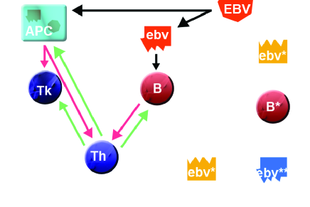
Figure 1: Circlets represent lymphocytes (T-cells in blue, B-cells in red); the red pentagon represents the Epstein-Barr Virus; irregular shapes are antigens (red), antibodies ebv* (yellow), or anti-anti-body ebv** (azure); the rectangular shape represents APCs or infected cells (healthy B-cells are not included). Different stages of the process are depicted in different colors: Infection (black arrows), Presentation (pink arrows), Activation (green arrows).

• Infection and presentation, [Regime $(0,0)$]. The virus starts the Lytic Cycle and infects permissive cells, producing antigens. The infected cells (via MHC-I) and the APCs (via MHC-II) present the processed antigen for specific T lymphocyte’s recognition. A resting CD4+ T-cell must be triggered via MHC-II present on either an APC or a (antigen-specific) B-cell (pink arrows in Figure 1) to become an activated $T_{H}$.

• Activation and response, [Regime $(1,1)$]. As the virus load overcomes the low dose tolerance of the lymphocytes, B-cells become fully activated by $T_{H}$ (green arrow in Fig. 1), so that they can now start to differentiate into memory cells and plasma cells producing antibodies; $T_{H}$ cells also provide the second signal, indirectly via APC, for a resting CD8+ T-cell. A resting CD8+ T-cell must be triggered by an APC via MHC-I (first signal, pink arrow in Fig. 1) and by $T_{H}$ (second signal, green arrow in Fig. 1) in order to become a $T_{K}$.
  The activated $T_{K}$ can now operate directly (yellow arrow in Fig. 2) on APC that is still in contact with the $T_{H}$, or that has been previously instructed. Meanwhile, the B-cell starts to produce antibodies (ebv*); such antibodies, being actually new antigens for the immune system, undergo an equivalent recognition process (yellow pattern in Fig. 2), so that they stimulate their specific B*-cells for T-cell presentation .

• Possible Learning, [Regime $(1,0)$]. The immune response eventually annihilates the antigenic load, the viral load ceases and $T_{K}$ cells, no longer stimulated, can undergo apoptosis. As for $B$ cells, they maintain a certain degree of stimulation (memory) even though of different nature with respect to the original one. In fact, as mentioned in Sec. 2.1, after activation, B* cells secrete antibodies (ebv**) that, being “complementary of the complementary” [31], resemble the original virus (ebv); as a result, they may act as signals themselves, that is, the antibodies ebv** sustain the stimulation of B cells .
  

  

  Figure 2: Kill and Memorize (yellow arrows). Agents are the same as in Fig. 1

  Now, according to the duration of the co-stimulation [Regime $(1,1)$] two alternative situations might happen:
  

  • Healthy Carrier State, HCS. If the Lytic Cycle has been interrupted within a relatively short time $t_{s}$ by the immune response, no associative learning between the production of $T_{K}$ cells and the production of B-cells is accomplished. The immune system has stored memory of the infection via memory cells and the EBV latency has established. The patient becomes a Healthy Carrier displaying specific memory healthy cells for those given antigens, as well as infected resting B cells in the Latent Cycle.
    

  • Chronic Fatigue Syndrome, CFS. The prolonged exposition to the (original) viral load (experimentally found to occur in the presence of large concentration of BRCF1 antigen) can lead to an associative learning between $T_{K}$ and B cells production. In fact, although $T_{K}$ are no longer directly stimulated by the antigen, the active state of $B$ cells can work itself as a surrogate stimulus. Namely, $T_{K}$ bypass the $T_{H}$ signal and interact directly with the MHC-II signal provided by B-cells as APC. This is consistent with [24], where it is reported that the BMLF1-specific CD8+ T-cell (which should only recognize the class MHC-I) gets active bypassing the necessary T-CD4+ indirect signal. This scenario would lead to a chronic activation state and it will be further discussed in the next Section.

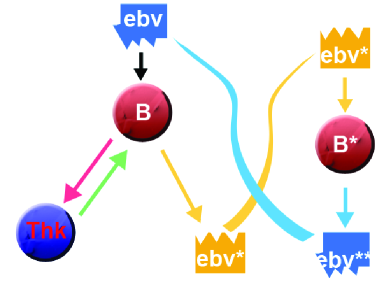
Figure 3: Learning. Agents are the same as in Fig. 1

To summarize, this is our proposal for the CFS etiology: a massive presence of BMLF1 antigens makes the clearance of the infection slow so that a long co-stimulation of BMLF1-specific B and $T_{K}$ cells takes place. During this stage a learning process occurs making $T_{K}$ cells able to detect the signal directly from $B$ cells, hence by-passing the direct stimulation from the antigen as well as from $T_{H}$. One can think at this situation as if $T_{K}$ assumed both killer and helper functions, that is as if it switched to a hybrid state.

In order to corroborate our speculation, we studied the dynamical properties of our model through analytical arguments and numerical simulations.

3.1 Formalization

In our interpretation, the viral load represents the external signal; when $s_{i}=+\infty$, the viral load is much bigger than threshold levels implied by low-dose tolerance [BA2, 32], conversely, when $s_{i}=0$, it is much lower. $T_{K}$ and $B$ cells belonging to clones specific for EBV antigen play as the neurons $\sigma_{1}$ and $\sigma_{2}$; the synapse $J$ represents the $T_{H}$ cell. Indeed, the $T_{H}$ can influence both $T_{K}$ and $B$ lymphocytes, via the sub-populations $T_{H_{1}}$ and $T_{H_{2}}$, respectively. Hence, the ”synapsis” should be thought of as a proper combination of $T_{H_{1}}$ and $T_{H_{2}}$, which results in a long relaxation time $\Theta$ (see Sec. 3.2).

Following [BA2, 32], the real size of the clone can be related to the time-average value of the representative spin, bounded in $[-1,1]$, by means of an exponential law:

$$M_{i}=\exp\left[\eta_{i}\left(\frac{m_{i}(t)+1}{2}\right)\right],$$ (4)

where $i=1,2$, and

$$W=\exp\left[\eta_{0}\left(\frac{w(t)+1}{2}\right)\right],$$ (5)

being $\eta_{i}$, $i=0,1,2$ a parameter that introduces the size of the pertaining population. These positions reproduce the chemical kinetics equation for the concentrations. Here we reasonably assume that the clones considered can be bounded by the same size $N=2\times 10^{11}$, so that $\eta_{i}=\log(N)$ [8].

Now, the AIM phase corresponds to a Regime $(1,1)$, where both $T_{K}$ and $B$ clones are stimulated by EBV antigens. The AIM phase is estimated to last from two weeks up to two months, so we choose $\tau$ in the interval $\tau\in[14;60]$ days.

Once the viral shedding has been interrupted by the immune responses, the $T_{K}$ clone is no longer stimulated, while the B-cell clone is still managing the memory of the infection (directly or Monte Carlothrough its conjugate specific antigen): This corresponds to the Regime $(0,1)$.
The two-steps evolution described here is a useful schematization for the analytical approach developed in the Appendix for the special cases $\beta=0$ and $\beta\rightarrow\infty$. More generally, the system of coupled differential equations (1) can be solved numerically for any value of $\beta$ and in the presence of continuous signals. In particular, while $s_{2}$ is still non-null over the whole range considered, $s_{1}$ can be chosen as exponentially decaying (being $t_{s}$ characteristic time for vanishing), in agreement with experimental findings [8].
Despite the system is well described by the stochastic dynamical equations (Eqs. (1)), we can improve the picture by including proper terms accounting for the collective behavior due to interaction with other lymphocytes and immune agents, that is, we mimic both quiescence induction and internal signaling to apoptosis by introducing further two small negative fields $|\epsilon_{1}|,|\epsilon_{2}|\ll 1$, in such a way that the effective fields are $\tilde{s}_{1}=s_{1}+\epsilon_{1}$ and $\tilde{s}_{2}=s_{2}+\epsilon_{2}$, respectively. We underline that the statistical mechanics reason for these small fields, whose effect would otherwise be negligible being them infinitesimal, is only breaking the gauge symmetry of the model, so to allow a quiescent state in the absence of signals.

3.2 On the mixed synapse and timescales

In our model the helper T-cell plays the role of the synapse. Upon activation, helper T cells differentiate in two major subtypes known as $T_{H_{1}}$ and $T_{H_{2}}$: Beyond other functions, the former maximizes the proliferation of cytotoxic CD8+, the latter stimulates B-cells into proliferation; also, they both produce cytokines which are aimed to their own proliferation and cross-regulate each other’s development and activity [8]. The net result is that, once the $T_{H}$ response begins to develop, it may get polarized in one of the two directions (either Type 1 or Type 2), due to auto-amplification and cross regulation [8].

Now, when the two sub-populations are completely balanced and small (corresponding to a quiescent state) none of the two prevails so that, in our equivalent model, there is no link between $B$ and $T_{K}$ ($w=0$) and no learning can be established among them (as intuitively $\Theta\to\infty$).
In general, one can assume that the characteristic timescales of lymphocyte growth are the same, independently of the particular type, that is, $T_{H}$, $T_{K}$ and $B$ cells require the same time $\tau$ to adjust their concentrations responding to a signal. However, in our model, the three agents considered feature different degrees of complexity: while $B$ and $T_{K}$ can be thought of as homogenous populations, $T_{H}$ displays inner degrees of freedom, being the combination of the two sub-populations $T_{H_{1}}$ and $T_{H_{2}}$. As a consequence, as the dynamics of $J$ tunes the unbalance between these populations (and they grow closely), its relaxation time $\Theta$ is assumed larger than $\tau$.

Conversely, when one of the two prevails the synapse is onset ($w\neq 0$), so that $B$ and $T_{K}$ can (indirectly) interact (still retaining a large timescale $\Theta$ compared to the single clone one $\tau$).
Hence, as envisaged by the scheme in Fig. 4 the central spin, playing the role of the synapse, can be thought of as a combination of two sub-populations. An effective way to relate the states of $T_{H_{1}}$ and $T_{H_{2}}$ with the overall state of $T_{H}$ is given by the following “average”, where we denote with $w_{1}$ and $w_{2}$ the “magnetizations” corresponding to the two sub-populations:

$$w=\frac{w_{1}w_{2}}{4}[w_{1}+w_{2}+|w_{1}|+|w_{2}|+|w_{1}-w_{2}|].$$ (6)

Indeed, this combination is in agreement with the immunological phenomenology and consistent with the model we are introducing: balanced, quiescent sub-populations correspond to $w=0$, a large unbalance in favor of any of the two sub-population means $w<0$, while when they are both stimulated we have a reinforcement effect ($w>0$).

The characteristic time for the response of $B$ and $T_{K}$ is taken to be $\tau\in[14,60]$, since the AIM phase is estimated to range from two weeks up to two months, while for our synapse we explore $\Theta$ starting from $\Theta\geq 90$ days (as the tunable parameter is the ratio $\tau/\Theta$, the previous choice does not modify the results). Furthermore, while the signal $s_{2}$ is constant, the signal $s_{1}$ (representing the real antigenic load) is taken exponentially decaying, in such a way that the effective time of its offset is $t_{s}$; similarly, in the analytical approach in the appendix the signal is active for a time $t\in[0,t_{s}]$, while the second regime holds for $t\in[t_{s},\infty)$, with $\tau<t_{s}<\Theta$. In any case we find that the value of $t_{s}$ crucially determines the final equilibrium state.

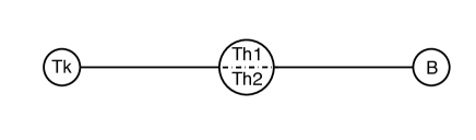
Figure 4: Schematic representation of the three-spins system considered, where the complex structure of the synapse (central spin) is explicitly envisaged.

3.3 The role of the latent and lytic cycles

In this section we want to deepen a way (typical of all herpes-viruses) which may further contribute to lengthen the hospitalization time of a CFS patient. In fact EBV, once the infection has been established in the host body, may hide away from immune recognition and opportunely switch between cycles of latency and cycles of lytic replication, somehow mirroring a switch between a quiescent and an active external stimulus (antigenic load) acting on the immune system. In fact, during latency, EBV mainly manages minimal tasks as inhibiting apoptosis and blocking viral lytic replication, while, during the lytic phase, EBV syntetizes proteins from many viral genes, allowing for nucleotide biosynthesis, RNA processing, viral DNA replication, etc.
As a consequence, within the framework based on ”Pavlov phenomenology” we are using to explain the transition from an AIM to a CFS scenario, these re-activations display significantly different outcomes in healthy carriers and in CFS patients. In fact, as shown in Fig. 5, for the formers, whose infection walked off quickly (toward an healthy carrier final state), sequential impulsive stimuli do not have particular consequences, while, for the latters, whose infection has been prolonged enough to allow the correlation via helpers, basically each time there is an impulsive reactivation, this thwarts the natural de-learning.

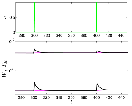
Figure 5: Upper panel: impulsive stimulus $s=s_{1}=s_{2}$ as a function of time; Lower panel: immune response in terms of concentration of $T_{K}$ (dark line) and of $T_{H}$ (bright line) for an healthy carrier (smaller values) and a CFS patient (higher values).

4 Results

The stochastic system of Eqs. (1)-(3) is solved numerically by means of standard Runge-Kutta packages for Matlab. For the sake of clearness, a fully analytical solution of the system is shown in the appendix, nonetheless, here it is worth introducing the whole set of observables we need to consider. In particular, we have to deal with averages and correlations:

$$w=\langle J\rangle_{\tau},\ m_{1}=\langle\sigma_{1}\rangle_{\tau},\ m_{2}=\langle\sigma_{2}\rangle_{\tau},m_{12}=\langle\sigma_{1}\sigma_{2}\rangle_{\tau},$$

$$m_{01}=\langle J\sigma_{1}\rangle_{\tau},\ m_{02}=\langle J\sigma_{2}\rangle_{\tau},\ m_{012}=\langle J\sigma_{1}\sigma_{2}\rangle_{\tau},\$$

where the average $\langle\cdot\rangle_{\tau}$, is meant over the time and over the ensamble due to ergodic hypothesis as explained in Sec. $2.4$ (see also the appendix). We set our initial conditions $\mathbf{m}(0)$ using concentrations expressed in cells/$\mu$L and keeping in mind that, in a healthy body, a given clone has an incidence of $1$ over $10^{5}$ cells with respect to the whole population; by using the normal values for lymphocytes concentrations and the relative translation in terms of magnetizations (see Eq. 4) reported in Tab. $1$, we get:

$$\mathbf{m}(0)=\left\{\begin{array}[]{l}w(0)\sim 0\\ m_{1}(0)=-0.971\\ m_{2}(0)=-0.938\\ m_{12}(0)=m_{1}(0)\cdot m_{2}(0)\\ m_{01}(0)=0\\ m_{02}(0)=0\\ m_{012}(0)=0\end{array}\right.$$ (7)

Notice that the initial value for the correlation $m_{12}$ as the product of the two concentrations $m_{1},m_{2}$ is a useful condition to initialize the evolution (implicitly assuming un-correlation), and we will use it during numerical integration.

Table 1: Data for initial conditions [8]. Notice that we do not specify the relative concentrations of $T_{H_{1}}$ and $T_{H_{2}}$,while we assume that their sum $T_{H}$ is, at rest, zero, i.e. $w\sim 0$, meaning a balance for the two sub-populations.

Agent	Concentration	$\%$	$M_{i}(0)$	$m_{i}(0)$
	(cells/$\mu$L)		(specific cells/$\mu$L)	(adimens.)
$T_{H}$	1000.50	46	0.010	-0.815
$T_{K}$	413.25	19	0.004	-0.971
$B$	500.25	23	0.005	-0.938

In order to recover the two cases of HSC patient and CFS patient, as reported in Sec. 2.3, we consider two different situations, corresponding to a short ($t_{s}=5$ days) and to a long ($t_{s}=100$ days) AIM phase, respectively. The other parameters holding for both patients are:

$$\tau=30,\ \Theta=90,$$

$$s_{1}=1000,\ s_{2}=e^{-(t-t_{s})/80},$$

$$\epsilon_{1}=-1.0,\ \epsilon_{2}=-1.0.$$

We also fix the level of noise as low ($\beta=6.5$), while later we will discuss the case of high noise.

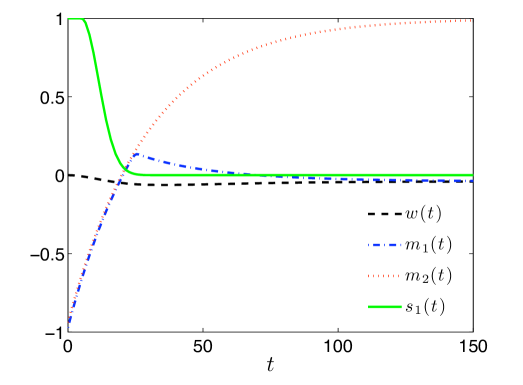
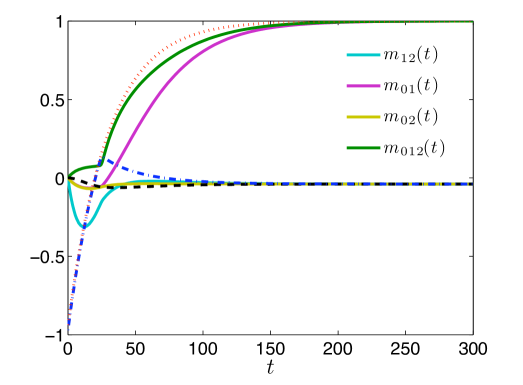
Figure 6: (Color online) Top panel: Averages $w$, $m_{1}$ $m_{2}$ and signal $s_{1}$ as a function of time (zoom on the early regime). Bottom panel: the same averages and their correlations as a function of time, as shown in the legends; time is measured in days. The signal on $T_{K}$ vanishes at around time $t_{s}=5$. The level of noise is low and fixed at $\beta=6.5$.

Patient 1: HSC Scenario.
As shown in Fig. 6, during the AIM phase ($t<t_{s}=5$ days), both signals $s_{1}$ and $s_{2}$ are active and, as responses, $m_{1}$, $m_{2}$ grow up, meaning that $T_{K}$ and $B$ clones are proliferating; the synapse also increases as both its afferent inputs are growing (correlations begin).
As the real viral load is diminishing, $T_{K}$ concentration decreases and finally reaches a value comparable with the initial one. Conversely, $B$ clones, being still stimulated, maintain high levels of concentration.

Patient 2: CFS Scenario.
As shown in Fig. 7, during the AIM phase ($t<t_{s}=100$ days), the concentrations of $B$, $T_{K}$ and $T_{H}$ increase as a result of a viral load ($s_{1},s_{2}>0$). This time, the signal on $T_{K}$ lasts long enough for $T_{K}$ and $T_{H}$ to reach high levels (both $\sim 10^{5}$ cells/$\mu$L) and, even when the signal is switched off their concentrations are much larger than the one pertaining to Patient 1.

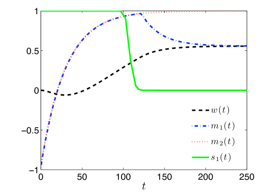
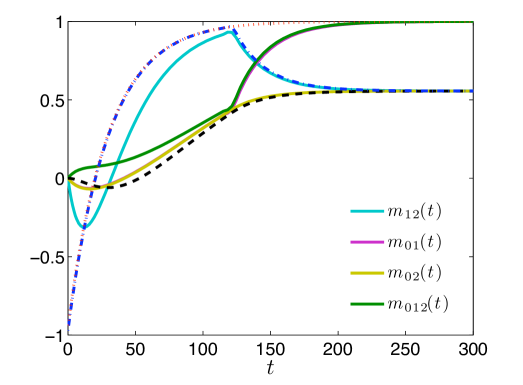
Figure 7: (Color online) Top panel: Averages $w$, $m_{1}$ $m_{2}$ and signal $s_{1}$ as a function of time (zoom on the early regime). Bottom panel: the same averages ad their correlations as a function of time, as shown in the legends; time is measured in days. The signal on $T_{K}$ vanishes at around time $t_{s}=100$. The level of noise is low and fixed at $\beta=6.5$.

The outcomes for the two cases are compared in Fig. 8, in terms of concentrations of $T_{H}$ and $T_{K}$. In particular, for Patient $1$, $T_{K}$ displays a maximum ($\sim 10^{3}$ cells/$\mu$L) at very short times and then relaxes to approximately $10^{2}$ cells/$\mu$L, while, for Patient $2$, $T_{K}$ reaches a higher maximum at longer times and then relaxes to approximately $10^{3}$ cells/$\mu$L.

Finally, when the level of noise is high, we expect that the effects due to interaction get more and more negligible. Indeed, in this model ”low” and ”high” levels of noise are not referred to a specific “critical value”, as this model does not break ergodicity by itself; conversely, since the noise level $\beta$ is coupled to the averaged energy in the system $E=\langle J\sigma_{1}\sigma_{2}\rangle$, their product defines the levels, i.e., either $\beta E>1$ , or $\beta E<1$. For instance, the case $\beta=0.8$ is shown in Fig. 9: notice that independently of the duration of $s_{1}$, both the averages $m_{1}$ and $m_{2}$ relax to small values.

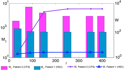
Figure 8: (Color on line) Evolution of the concentrations of $T_{K}$ cells (histogram, left vertical axis) and of $T_{H}$ cells (curves, right vertical axis) for the two patients considered in the case of small noise.

To summarize, according to the duration of the AIM phase, which is in turn related to the success of the EBV strategy (Sec. 2.3), we can get two possible scenarios. If the AIM phase is rather fast, when the viral load has vanished, $B$ cells are continuously activated, while the concentration of $T_{K}$ cells recovers normal values hence we reach an equilibrium state corresponding to an healthy carrier state.
Conversely, if AIM phase is prolonged, a strong correlation between the active $B$ and $T_{K}$ lymphocytes can be accomplished; as a result, when the viral load has vanished, again $B$ cells are continuously activated but $T_{K}$ lymphocytes can maintain high concentrations. This is the actualization of a conditional reflex and, from a mathematically point of view it arises from the large correlation $w$ stored, able to sustain the active status of $T_{K}$.

Figure 9: (Color on line) Averages $w$, $m_{1}$ $m_{2}$ and signal $s_{1}$ (see the legend) as a function of time for Patient 1 (top panel) and Patient 2 (bottom panel). The level of noise is low and fixed at $\beta=0.8$.

5 Conclusion and Discussion

The Chronic Fatigue Syndrome (CFS) has been studied for almost thirty years in the whole biological, medical and psychological world, being identified with tens of medical terms; as well, a full consensus on its genesis, physiopathology and treatment has not been reached yet.

It is just the lack of a clear-cut picture that makes theoretical models very useful tools in order to get information about the possible causes of this disease. The present work aims to take advantage of the statistical-mechanics lenses to investigate why and how the CFS may establish. Of course, the model cannot simulate the whole immune system, which is much too complicated, rather, it has to get a compromise between simplification and inclusion of most important characters, the latter chosen according to experimental facts.

Our framework is inspired by the well-known conditional reflex phenomenon in neurobiology, which, from a statistical mechanics perspective, can be recovered in terms of thermodynamic relaxation of complex systems [27]. Given two agents (e.g. two neurons or $B$ and $T_{K}$ lymphocytes) and a coupling (e.g. the synapse or the $T_{H}$ lymphocytes) joining them, provided that two agents are contemporary stimulated by two related signals (e.g. neural stimuli or antigens), then, even though one of the signal is switched off, the two agents may remain both active; this realizes the so-called ”associative learning”.
More precisely, along this analogy, we find that, if the Epstein-Barr virus infection is prolonged in time, $T_{K}$ and B cells can reach high values of concentration, moreover, the latter have time enough to produce the image ebv**. As a result, when the (real) viral load has vanished, B cells are still stimulated, while $T_{K}$ may maintain high concentration levels since they have learnt the correlation between presence-of-antigen and B-activation. Interestingly, this learning process also implies that $T_{K}$ can get activated by-passing the signal from $T_{H}$ cells and this has been recently found experimentally.
Therefore, our model and our analysis suggest that the CFS, meant as a chronically active immune state, can arise from an associative-learning phenomenon.
As a consequence, our results clarify why some individuals are affected by this disease while some other are not, why some infections may drive it (we investigated the case of EBV) while some other may not: Within our framework, the genesis of this chronically active state is guided by the ability of a particular virus (e.g. EBV) to elude immuno-surveillance for a larger timescale with respect to the standard ones set by the other antigens. Clearly, as EBV-infected patients may solve the infection in a wide range of times, the ones with the infection lasting for too long are natural candidates to develop CFS. Likewise, other pathogens, such as Citomegalovirus, can drive a long-term infection, hence allowing correlations and non-trivial outcomes.
Furthermore, our suggestion may be exploited in future experiments in order to shed light on the etiology of this syndrome; indeed, at least at a theoretical physics level, unlearning processes are actually possible.

Finally, it is worth stressing the ”guide role” of statistical mechanics when modeling biological systems: in fact this approach, constraining the system to respect thermodynamics, can provide a working picture possibly inspiring experimental paths. In this sense, relying on natural and minimal assumptions, we evidence the emergence of a subtle role by $T_{K}$ (able to bypass a standard double signal activation provided by antigen plus helpers), and, indeed, we found its consistency with experimental data. In fact in [33], it has been documented that a CD8+ T receptors, that normally recognize MHC-I signals can exhibit dual specificity recognizing also an antigen in the context of the MHC-II.

6 Appendix: Evolution toward steady states of the system

The system, whose dynamics is investigated Monte Carlothrough the paper, can be resumed as follows:
$\sigma_{1}$ and $\sigma_{2}$ are the effector cells (i.e., neurons in the neurobiology counterpart), while $J_{12}$ is the helper cell (synapse); moreover we name $s_{1},s_{2}$ the antigens (external fields) acting respectively on $\sigma_{1},\sigma_{2}$. Lymphocytes can be either active or quiescent ($\sigma_{i}=\pm 1$) and can be grouped into clones. Each clone is made up of a huge amount cells expressing the same idiotipicity and it is expected to be homogeneous. Analogously, in statistical mechanics, we can apply the ergodic hypothesis, and move from their time-average to their ensemble average, using equivalently

$$m_{i} = \int_{0}^{T}\sigma_{i}(t)dt=\frac{1}{N}\sum_{j=1}^{N}\sigma_{i}^{(j)},$$ (8)

$$w = \int_{0}^{T}J(t)dt=\frac{1}{N}\sum_{j=1}^{N}J^{(j)},$$ (9)

where $i=1,2$ and the index $(j)$ denotes the element within the clone considered. We also stress that both the support $T$ of the integral and the size $N$ of the clone are large: In the limit of $T,N\to\infty$ the variable $m\in\mathbb{R}$ hence allowing a continuous description in terms of Langevin equations.
Each of the variable experiences the same structure of (external/internal) fields, namely (calling $\sigma_{3}=J_{12}$ to preserve the symmetry)

$$\langle\sigma_{i}\rangle=\langle\tanh\Big{(}\beta\sigma_{i+1}\sigma_{i+2}+s_{i}\Big{)}\rangle=a_{i}+b_{i}\langle\sigma_{i+1}\sigma_{i+2}\rangle,$$ (10)

where

$$a_{i} = \frac{1}{2}\left[\tanh(\beta+s_{i})+\tanh(-\beta+s_{i})\right],$$ (11)

$$b_{i} = \frac{1}{2}\left[\tanh(\beta+s_{i})-\tanh(-\beta+s_{i})\right].$$ (12)

Overall, we have the following system

$$\langle\sigma_{1}\rangle = \langle\tanh(\beta J\sigma_{2}+s_{1})\rangle=\tanh(\beta J\langle\sigma_{2}\rangle+s_{1}),$$ (13)

$$\langle J\rangle = \langle\tanh(\beta\sigma_{1}\sigma_{2})\rangle=\langle\sigma_{1}\sigma_{2}\rangle\tanh(\beta),$$ (14)

$$\langle\sigma_{2}\rangle = \langle\tanh(\beta J\sigma_{1}+s_{2})\rangle=\tanh(\beta J\langle\sigma_{1}\rangle+s_{1},$$ (15)

where in the last passage of eq.s (13,15) we assumed the mean field approximation, namely

$$\langle f(m)\rangle\sim f(\langle m\rangle),$$

as we are interested in the average behavior.
The time scale of $J$ is $\Theta\ll\tau$, being $\tau$ the time scale of the $\sigma$ and we pose $\frac{1}{\Theta}+\frac{1}{\tau}=\frac{1}{\tau^{\prime}}$, $\frac{2}{\tau}+\frac{1}{\Theta}=\frac{1}{\tau^{\prime\prime}}$. For the sake of clearness, while we used the milder notation with $m,w$ in the text to lighten the notation, here we develop the whole theory using the brackets. The averages are assumed to evolve according to

$$\tau\frac{d\langle\sigma_{1}\rangle}{dt} = -\langle\sigma_{1}\rangle+a_{1}+b_{1}\langle J\sigma_{2}\rangle,$$ (16)

$$\Theta\frac{d\langle J\rangle}{dt} = -\langle J\rangle+\tanh(\beta)\langle\sigma_{1}\sigma_{2}\rangle,$$ (17)

$$\tau\frac{d\langle\sigma_{2}\rangle}{dt} = -\langle\sigma_{2}\rangle+a_{2}+b_{2}\langle J\sigma_{1}\rangle,$$ (18)

while the correlations evolve according to

$$\frac{d\langle\sigma_{1}\sigma_{2}\rangle}{dt} = \frac{-2}{\tau}\langle\sigma_{1}\sigma_{2}\rangle+\frac{1}{\Theta}\Big{(}a_{1}\langle\sigma_{2}\rangle+b_{1}\langle J\rangle+a_{2}\langle\sigma_{1}\rangle+b_{2}\langle J\rangle\Big{)},$$ (19)

$$\frac{d\langle J\sigma_{1}\rangle}{dt} = \frac{-1}{\tau^{\prime}}\langle J\sigma_{1}\rangle+\frac{1}{\Theta}\tanh(\beta)\langle\sigma_{2}\rangle+\frac{1}{\tau}\Big{(}a_{1}\langle J\rangle+b_{1}\langle\sigma_{2}\rangle\Big{)},$$ (20)

$$\frac{d\langle J\sigma_{2}\rangle}{dt} = \frac{-1}{\tau^{\prime}}\langle J\sigma_{2}\rangle+\frac{1}{\Theta}\tanh(\beta)\langle\sigma_{1}\rangle+\frac{1}{\tau}\Big{(}a_{2}\langle J\rangle+b_{2}\langle\sigma_{1}\rangle\Big{)},$$ (21)

$$\frac{d\langle J\sigma_{1}\sigma_{2}\rangle}{dt} = \frac{-2}{\tau^{\prime\prime}}\langle J\sigma_{1}\sigma_{2}\rangle+\frac{1}{\Theta}\tanh(\beta)+\frac{1}{\tau}\Big{(}a_{1}\langle J\sigma_{2}\rangle+b_{1}+a_{2}\langle J\sigma_{1}\rangle+b_{2}\Big{)},$$ (22)

as in standard off-equilibrium statistical mechanics.
The source of $\langle\sigma_{1}\rangle$ and of $\langle\sigma_{2}\rangle$ are $s_{1}$ and $s_{2}$, respectively, while the source for $\langle J\rangle$ is the internal correlation $\langle\sigma_{1}\sigma_{2}\rangle$.
According to the mutual value of $s_{1}$ and $s_{2}$, such a system experiences different regimes, whose dynamics we are going to analyze.

6.1 Regime $s_{1}=0,s_{2}=0$: No signalling.

Langevin dynamics reduces to

$$\Theta\frac{d\langle J\rangle}{dt} = -\langle J\rangle+\tanh(\beta)\langle\sigma_{1}\sigma_{2}\rangle,$$ (23)

$$\tau\frac{d\langle\sigma_{1}\rangle}{dt} = -\langle\sigma_{1}\rangle+\tanh(\beta)\langle J\sigma_{2}\rangle,$$ (24)

$$\tau\frac{d\langle\sigma_{2}\rangle}{dt} = -\langle\sigma_{2}\rangle+\tanh(\beta)\langle J\sigma_{1}\rangle,$$ (25)

$$\frac{d\langle\sigma_{1}\sigma_{2}\rangle}{dt} = \frac{1}{\tau}\Big{(}-2\langle\sigma_{1}\sigma_{2}\rangle+2\tanh(\beta)\langle J\rangle\Big{)},$$ (26)

$$\frac{d\langle J\sigma_{1}\rangle}{dt} = -\frac{1}{\tau^{\prime}}\langle J\sigma_{1}\rangle+\frac{1}{\tau^{\prime}}\tanh(\beta)\langle\sigma_{2}\rangle,$$ (27)

$$\frac{d\langle J\sigma_{2}\rangle}{dt} = -\frac{1}{\tau^{\prime}}\langle J\sigma_{2}\rangle+\frac{1}{\tau^{\prime}}\tanh(\beta)\langle\sigma_{1}\rangle,$$ (28)

$$\frac{d\langle J\sigma_{1}\sigma_{2}\rangle}{dt} = -\frac{1}{\tau^{\prime\prime}}\langle J\sigma_{1}\sigma_{2}\rangle+\frac{1}{\tau^{\prime\prime}}\tanh(\beta).$$ (29)

As it is immediate to see, the global dynamics spreads over four different independent sub-dynamics, namely $\langle\sigma_{1}\rangle\Longleftrightarrow\langle J\sigma_{2}\rangle$, $\langle\sigma_{2}\rangle\Longleftrightarrow\langle J\sigma_{1}\rangle$, $\langle\sigma_{1}\sigma_{2}\rangle\Longleftrightarrow\langle J\rangle$, $\langle J\sigma_{1}\sigma_{2}\rangle$, whose asymptotic regime is given by $\langle J\rangle=\langle\sigma_{1}\sigma_{2}\rangle=0$, $\langle\sigma_{1}\rangle=\langle J\sigma_{2}\rangle=0$, $\langle\sigma_{2}\rangle=\langle J\sigma_{1}\rangle=0$, $\langle J\sigma_{1}\sigma_{2}\rangle=\tanh(\beta)$.
The general solution of the problem can be obtained coupling the four different sub-dynamics.
By the first set we get

$$\frac{d\langle J\rangle}{dt} = -\frac{1}{\Theta}\langle J\rangle+\frac{\tanh(\beta)}{\Theta}\langle\sigma_{1}\sigma_{2}\rangle$$ (30)

$$\frac{d\langle\sigma_{1}\sigma_{2}\rangle}{dt} = -\frac{2}{\tau}\langle\sigma_{1}\sigma_{2}\rangle+\frac{2\tanh(\beta)}{\tau}\langle J\rangle.$$ (31)

whose matrix can be written as

$$\left(\begin{array}[]{c c }1/\Theta&-\tanh(\beta)/\Theta\\ -2\tanh(\beta)/\Theta&2/\Theta\\ \end{array}\right).$$

We can diagonalize the sub-dynamics by looking for solutions as linear combinations as

$$Y(t)=a\langle J(t)\rangle+b\langle\sigma_{1}(t)\sigma_{2}(t)\rangle,$$ (32)

and we can associate to this new variable a characteristic timescale $\bar{\tau}$ as

$$\bar{\tau}\frac{dY}{dt}=-Y\Longrightarrow\frac{a\bar{\tau}}{\Theta}\Big{(}-\langle J\rangle+\tanh(\beta)\langle\sigma_{1}\sigma_{2}\rangle\Big{)}$$

$$+ \frac{2b\bar{\tau}}{\tau}\Big{(}-\langle\sigma_{1}\sigma_{2}\rangle+\tanh(\beta)\langle J\rangle\Big{)}=-a\langle J\rangle-b\langle\sigma_{1}\sigma_{2}\rangle.$$

Namely we get the system

$$\Big{(}1-\frac{\bar{\tau}}{\Theta}\Big{)}+2\frac{\bar{\tau}}{\tau}\tanh(\beta)b = 0$$ (34)

$$\frac{\bar{\tau}}{\Theta}\tanh(\beta)a+\Big{(}1-2\frac{\bar{\tau}}{\Theta}\Big{)}b = 0.$$ (35)

Let us work out $\bar{\tau}(\beta)$:

$$\left(\frac{1}{\bar{\tau}}\right)^{2}-\left(\frac{1}{\bar{\tau}}\right)\left[\frac{1}{\Theta}\frac{2}{\tau}\right]+\frac{2}{\tau\Theta}\frac{1}{\cosh^{2}(\beta)}=0,$$ (36)

whose roots are

$$\frac{1}{\bar{\tau}_{1,2}\left(\beta\right)}=\frac{1}{2}\left[\frac{1}{\Theta}+\frac{2}{\tau}\pm\sqrt{\left(\frac{1}{\Theta}+\frac{2}{\tau}\right)^{2}-\frac{8}{\tau\Theta\cosh^{2}(\beta)}}\right].$$ (37)

Now we have to solve for $a,b$ in $Y=a\langle J\rangle+b\langle\sigma_{1}\sigma_{2}\rangle$. We can define $a=2c\frac{\bar{\tau}}{\Theta}\tanh(\beta)$, $b=-c(1-\frac{\bar{\tau}}{\Theta})$, by which

$$Y_{0}(t) = c_{0}\Big{(}2\frac{\bar{\tau}_{1}}{\tau}\tanh(\beta)\langle J\rangle-(1-\frac{\bar{\tau}_{1}}{\Theta})\langle\sigma_{1}\sigma_{2}\rangle\Big{)}$$ (38)

$$Y_{12}(t) = c_{12}\Big{(}2\frac{\bar{\tau}_{2}}{\tau}\tanh(\beta)\langle J\rangle-(1-\frac{\bar{\tau}_{2}}{\Theta})\langle\sigma_{1}\sigma_{2}\rangle\Big{)},$$ (39)

on which we can fix $c_{0},c_{12}$ as $c_{0}=\tau/2\bar{\tau}_{1}\tanh(\beta)$, $c_{12}=-1/(1-\bar{\tau}_{2}/\Theta)$. From eq.(36) we get

$$\tanh(\beta)=\sqrt{\frac{\tau\Theta}{2}}\sqrt{\left(\frac{1}{\bar{\tau}}-\frac{1}{\Theta}\right)\left(\frac{1}{\bar{\tau}}-\frac{2}{\tau}\right)}$$

and we can solve for $Y_{0},Y_{12}$:

$$Y_{0}(t) = \langle J\rangle+\sqrt{\frac{\tau}{2\Theta}}\sqrt{\frac{\frac{1}{\Theta}-\frac{1}{\bar{\tau}_{1}}}{\frac{2}{\tau}-\frac{1}{\bar{\tau}_{1}}}}\langle\sigma_{1}\sigma_{2}\rangle,$$ (40)

$$Y_{12}(t) = \langle\sigma_{1}\sigma_{2}\rangle-\sqrt{\frac{2\Theta}{\tau}}\sqrt{\frac{\frac{1}{\bar{\tau}_{2}}-\frac{2}{\tau}}{\frac{1}{\bar{\tau}_{2}}-\frac{1}{\Theta}}}\langle J\rangle,$$ (41)

so we get the form

$$Y_{0}(t) = \langle J(t)\rangle+A_{0}\langle\sigma_{1}(t)\sigma_{2}(t)\rangle,$$ (42)

$$Y_{12}(t) = \langle\sigma_{1}(t)\sigma_{2}(t)\rangle-A_{12}\langle J(t)\rangle,$$ (43)

with

$$A_{0}=\sqrt{\frac{\tau}{2\Theta}}\sqrt{\frac{\frac{1}{\Theta}-\frac{1}{\bar{\tau}_{1}}}{\frac{2}{\tau}-\frac{1}{\bar{\tau}_{1}}}},\ \ \ A_{12}=\sqrt{\frac{2\Theta}{\tau}}\sqrt{\frac{\frac{1}{\bar{\tau}_{2}}-\frac{2}{\tau}}{\frac{1}{\bar{\tau}_{2}}-\frac{1}{\Theta}}}.$$

By the eigenvalues found in eq.s(37) we can build the eigenvectors $V_{1}=(V_{11},V_{12}),V_{2}=(V_{21},V_{22})$ as

$$V_{11}=\tanh(\beta)/\Theta,\ V_{12}=\left(\frac{1}{2T}-\frac{1}{\tau}-\frac{1}{2}\sqrt{\Delta}\right),$$

$$V_{21}=\tanh(\beta)/\Theta,\ V_{22}=\left(\frac{1}{2\Theta}-\frac{1}{\tau}+\frac{1}{2}\sqrt{\Delta}\right),$$

being $\Delta=(1/\Theta+2/\tau)^{2}-\frac{8}{\Theta\tau\cosh^{2}(\beta)}$, by which, finally we get

$$\langle J(t)\rangle = C_{1}V_{11}e^{-\frac{t}{\bar{\tau}_{1}}}+C_{2}V_{12}e^{-\frac{t}{\bar{\tau}_{2}}},$$ (44)

$$\langle\sigma_{1}(t)\sigma_{2}(t)\rangle = C1V_{21}e^{-\frac{t}{\bar{\tau}_{1}}}+C_{2}V_{22}e^{-\frac{t}{\bar{\tau}_{2}}}.$$ (45)

By the second set we get

$$\tau\frac{d\langle\sigma_{1}\rangle}{dt} = -\langle\sigma_{1}\rangle+\tanh(\beta)\langle J\sigma_{2}\rangle,$$ (46)

$$\tau^{\prime}\frac{d\langle J\sigma_{2}\rangle}{dt} = -\langle J\sigma_{2}\rangle+\tanh(\beta)\langle\sigma_{1}\rangle.$$ (47)

whose matrix can be written as

$$\left(\begin{array}[]{c c }1/\tau&-\tanh(\beta)/\tau\\ -\tanh(\beta)/\tau^{\prime}&1/\tau^{\prime}\\ \end{array}\right).$$

Again we can write a solution in the general form $Y(t)=a\langle\sigma_{1}\rangle+b\langle J\sigma_{2}\rangle$ and label $\bar{\tau}$ its characteristic timescale such that

$$\bar{\tau}\frac{dY}{dt}=-Y$$

$$\Longrightarrow\frac{\bar{\tau}}{\tau}a\Big{(}-\langle\sigma_{1}\rangle+\tanh(\beta)\langle J\sigma_{2}\rangle\Big{)}+\frac{\bar{\tau}}{\tau^{\prime}}b\Big{(}-\langle J\sigma_{2}\rangle+\tanh(\beta)\langle\sigma_{1}\rangle\Big{)}=$$

$$=-a\langle\sigma_{1}\rangle+b\langle J\sigma_{2}\rangle,$$

and write the system

$$(1-\frac{\bar{\tau}}{\tau})a+\frac{\bar{\tau}}{\tau^{\prime}}\tanh(\beta)b = 0,$$ (48)

$$\frac{\bar{\tau}}{\tau}\tanh(\beta)a+(1-\frac{\bar{\tau}}{\tau^{\prime}})b = 0.$$ (49)

Again we can find the eigenvalues $\bar{\tau}^{-1}_{1,2}(\beta)$ as

$$\frac{1}{\bar{\tau}_{1,2}(\beta)}=\frac{1}{2}\Big{(}\frac{1}{\tau}+\frac{1}{\tau^{\prime}}\pm\sqrt{(\frac{1}{\tau}+\frac{1}{\tau^{\prime}})^{2}-\frac{4}{\tau\tau^{\prime}}(1-\tanh^{2}(\beta))}\Big{)}$$ (50)

and write the general solution in the form

$$\langle\sigma_{1}(t)\rangle = \frac{C_{1}\tanh(\beta)}{\tau}e^{-\frac{t}{\bar{\tau}_{1}}}-\frac{C_{2}\tanh(\beta)}{\tau}e^{-\frac{t}{\bar{\tau}_{2}}},$$ (51)

$$\langle J\sigma_{2}(t)\rangle = -\frac{C_{1}}{2}(\frac{1}{\Theta}-\sqrt{\Delta})e^{-\frac{t}{\bar{\tau}_{1}}}-\frac{C_{2}}{2}(\frac{1}{\Theta}-\sqrt{\Delta})e^{-\frac{t}{\bar{\tau}_{2}}},$$ (52)

$\Delta$ being $(1/\tau+1/\tau^{\prime})^{2}-(4/\tau\tau^{\prime})(1-\tanh(\beta))$.

For the two other subsystems we can proceed exactly as we did so far and verify that, even though on different timescales, all the observables (magnetizations and correlations) converge to zero.

6.2 Regime $s_{1}=0,s_{2}=\infty$: One infinite signal.

Let us start with the following conditions: $s_{1}=0,s_{2}=\infty$, then we have $a_{1}=0,b_{1}=\tanh(\beta),a_{2}=1,b_{2}=0$ and the evolution of the system can be written as

$$\Theta\frac{d\langle J\rangle}{dt} = -\langle J\rangle+\tanh(\beta)\langle\sigma_{1}\sigma_{2}\rangle,$$ (53)

$$\tau\frac{d\langle\sigma_{1}\rangle}{dt} = -\langle\sigma_{1}\rangle+\tanh(\beta)\langle J\sigma_{2}\rangle,$$ (54)

$$\tau\frac{d\langle\sigma_{2}\rangle}{dt} = -\langle\sigma_{2}\rangle+1,$$ (55)

$$\tau\frac{d\langle\sigma_{1}\sigma_{2}\rangle}{dt} = -2\langle\sigma_{1}\sigma_{2}\rangle+\tanh(\beta)\langle J\rangle+\langle\sigma_{1}\rangle,$$ (56)

$$\frac{d\langle J\sigma_{1}\rangle}{dt} = -\frac{1}{\tau^{\prime}}\langle J\sigma_{1}\rangle+\frac{1}{\tau^{\prime}}\tanh(\beta)\langle\sigma_{2}\rangle,$$ (57)

$$\frac{d\langle J\sigma_{2}\rangle}{dt} = -\frac{1}{\tau^{\prime}}\langle J\sigma_{2}\rangle+\frac{1}{\Theta}\tanh(\beta)\langle\sigma_{1}\rangle+\frac{1}{\tau}\langle J\rangle,$$ (58)

$$\frac{d\langle J\sigma_{1}\sigma_{2}\rangle}{dt} = -\frac{1}{\tau^{\prime\prime}}\langle J\sigma_{1}\sigma_{2}\rangle+\frac{1}{\tau}\langle J\sigma_{1}\rangle+\frac{1}{\tau^{\prime}}\tanh(\beta).$$ (59)

The presence of a signal in the second channel bridges the two sets $(\langle\sigma_{1}(t)\rangle,\langle J\sigma_{2}(t)\rangle)$ and $(\langle\sigma_{1}(t)\sigma_{2}(t)\rangle,\langle J(t)\rangle)$ such that the latter, if the system has experienced the field enough time to learn correlations, will assume high values: a signal in the second channel may induce a response even in the first channel.

Let us divide the system again by considering the following, natural sub-dynamics

$$\Theta\frac{d\langle J\rangle}{dt} = -\langle J\rangle+\tanh(\beta)\langle\sigma_{1}\sigma_{2}\rangle,$$ (60)

$$\tau\frac{d\langle\sigma_{1}\sigma_{2}\rangle}{dt} = -2\langle\sigma_{1}\sigma_{2}\rangle+2\tanh(\beta)\langle J\rangle$$ (61)

$$+ [\langle\sigma_{1}\rangle-\tanh(\beta)\langle J(t)\rangle].$$

We observe that the term $[\langle\sigma_{1}\rangle-\tanh(\beta)\langle J(t)\rangle]$ is a novelty with respect to the same equations in the regime $s_{1}=0,s_{2}=0$ and represents the ”unlearning source”: if the conditional reflex (which we are going to introduce) is not reinforced, it will tend to vanish.
The source of such a conditional reflex can be found by looking at the other subsystem, namely

$$\tau\frac{d\langle\sigma_{1}\rangle}{dt} = -\langle\sigma_{1}\rangle+\tanh(\beta)\langle J\sigma_{2}\rangle,$$ (62)

$$\frac{d\langle J\sigma_{2}\rangle}{dt} = -\frac{1}{\tau^{\prime}}\langle J\sigma_{2}\rangle+\frac{1}{\tau^{\prime}}\tanh(\beta)\langle\sigma_{1}\rangle$$ (63)

$$+ \frac{1}{\tau}[\langle J\rangle-\tanh(\beta)\langle\sigma_{1}\rangle].$$

In fact, the new term $[\langle J\rangle-\tanh(\beta)\langle\sigma_{1}\rangle]$, namely the source of the conditional reflex, is a learning term as it couples the slow channel $(\langle J\rangle,\langle\sigma_{1}\sigma_{2}\rangle)$ with the fast one $(\langle\sigma_{1}\rangle,\langle J\sigma_{2}\rangle)$.
We can now start studying the dynamics in this regime by considering the sub-dynamics of ($\langle J\rangle$, $\langle\sigma_{1}\rangle$, $\langle\sigma_{1}\sigma_{2}\rangle$, $\langle J\sigma_{2}\rangle$), whose dynamical system reads off as

$$\tau\frac{d\langle\sigma_{1}\rangle}{dt} = -\langle\sigma_{1}\rangle+\tanh(\beta)\langle J\sigma_{2}\rangle,$$ (64)

$$\Theta\frac{d\langle J\rangle}{dt} = -\langle J\rangle+\tanh(\beta)\langle\sigma_{1}\sigma_{2}\rangle,$$ (65)

$$\tau\frac{d\langle\sigma_{1}\sigma_{2}\rangle}{dt} = -2\langle\sigma_{1}\sigma_{2}\rangle+\tanh(\beta)\langle J\rangle+\langle\sigma_{1}\rangle,$$ (66)

$$\frac{d\langle J\sigma_{2}\rangle}{dt} = -\frac{1}{\tau^{\prime}}\langle J\sigma_{2}\rangle+\frac{1}{\tau}\langle J\rangle+\frac{1}{\Theta}\tanh(\beta)\langle\sigma_{1}\rangle.$$ (67)

The associated matrix can be written as

$$\left(\begin{array}[]{c c c c}1/\tau&0&0&-\tanh(\beta)/\tau\\ 0&1/\Theta&-\tanh(\beta)/\Theta&0\\ -\frac{1}{\tau}&-\frac{1}{\tau}\tanh(\beta)&\frac{2}{\tau}&0\\ -\frac{1}{\Theta}\tanh(\beta)&-\frac{1}{\tau}&0&\frac{1}{\tau^{\prime}}\end{array}\right).$$

We can diagonalize the dynamics and look for solutions as linear combinations like $Y(t)=a\langle\sigma_{1}\rangle+b\langle J\rangle+c\langle\sigma_{1}\sigma_{2}\rangle+d\langle J\sigma_{2}\rangle$, associating to this variable its characteristic timescale $\bar{\tau}\Leftrightarrow Y$, and proceed as for the former regime.
Skipping all the calculations for the sake of brevity we report only the solution

$$\langle\sigma_{1}(t)\rangle=c_{1}x_{1}e^{-\frac{t}{\bar{\tau}_{1}}}+c_{2}x^{{}^{\prime}}_{1}e^{-\frac{t}{\bar{\tau}_{2}}}+c_{3}x_{1}^{{}^{\prime\prime}}e^{-\frac{t}{\bar{\tau}_{3}}}+c_{4}x_{1}^{{}^{\prime\prime\prime}}e^{-\frac{t}{\bar{\tau}_{4}}},$$

$$\langle J(t)\rangle=c_{1}x_{2}e^{-\frac{t}{\bar{\tau}_{1}}}+c_{2}x_{2}^{{}^{\prime}}e^{-\frac{t}{\bar{\tau}_{2}}}+c_{3}x_{2}^{{}^{\prime\prime}}e^{-\frac{t}{\bar{\tau}_{3}}}+c_{4}x_{2}^{{}^{\prime\prime\prime}}e^{-\frac{t}{\bar{\tau}_{4}}},$$

$$\langle\sigma_{1}(t)\sigma_{2}(t)\rangle=c_{1}x_{3}e^{-\frac{t}{\bar{\tau}_{1}}}+c_{2}x_{3}^{{}^{\prime}}e^{-\frac{t}{\bar{\tau}_{2}}}+c_{3}x_{3}^{{}^{\prime\prime}}e^{-\frac{t}{\bar{\tau}_{3}}}+c_{4}x_{3}^{{}^{\prime\prime\prime}}e^{-\frac{t}{\bar{\tau}_{4}}},\$$

$$\langle J(t)\sigma_{2}(t)\rangle=c_{1}x_{4}e^{-\frac{t}{\bar{\tau}_{1}}}+c_{2}x_{4}^{{}^{\prime}}e^{-\frac{t}{\bar{\tau}_{2}}}+c_{3}x_{4}^{{}^{\prime\prime}}e^{-\frac{t}{\bar{\tau}_{3}}}+c_{4}x_{4}^{{}^{\prime\prime\prime}}e^{-\frac{t}{\bar{\tau}_{4}}},$$

all the $x$’s being the component of the following eigenvectors $V_{1}=(x_{1},x_{2},x_{3},x_{4})$, $V_{2}=(x_{1}^{{}^{\prime}},x_{2}^{{}^{\prime}},x_{3}^{{}^{\prime}},x_{3}^{{}^{\prime}})$, $V_{3}=(x_{1}^{{}^{\prime\prime}},x_{2}^{{}^{\prime\prime}},x_{3}^{{}^{\prime\prime}},x_{3}^{{}^{\prime\prime}})$, $V_{4}=(x_{1}^{{}^{\prime\prime\prime}},x_{2}^{{}^{\prime\prime\prime}},x_{3}^{{}^{\prime\prime\prime}},x_{3}^{{}^{\prime\prime\prime}})$:

$$x_{1} = \frac{1}{\tau}\tanh(\beta),$$

$$x_{2} = \frac{1}{2}\Big{(}\frac{1}{\tau}-\frac{1}{\Theta}-\sqrt{\Delta}\Big{)},$$

$$x_{3} = \frac{1}{\tau}\tanh(\beta),$$

$$x_{4} = \frac{1}{2}\Big{(}\frac{1}{\tau}-\frac{1}{\Theta}-\sqrt{\Delta}\Big{)},$$

$$x^{{}^{\prime}}_{1} = \frac{1}{\tau}\tanh(\beta),$$

$$x^{{}^{\prime}}_{2} = \frac{1}{2}\Big{(}\frac{1}{\tau}-\frac{1}{\Theta}+\sqrt{\Delta}\Big{)},$$

$$x^{{}^{\prime}}_{3} = \frac{1}{\tau}\tanh(\beta),$$

$$x^{{}^{\prime}}_{4} = \frac{1}{2}\Big{(}\frac{1}{\tau}-\frac{1}{\Theta}+\sqrt{\Delta}\Big{)},$$

$$x^{{}^{\prime\prime}}_{1} = \frac{1}{\tau}\tanh(\beta),$$

$$x^{{}^{\prime\prime}}_{2} = \frac{1}{2}\Big{(}\frac{1}{\tau}-\frac{1}{\Theta}+\sqrt{\Delta}\Big{)},$$

$$x^{{}^{\prime\prime}}_{3} = \frac{\Theta}{\tanh(\beta)}\Big{[}\frac{3}{2\tau\Theta}-\frac{1}{2\Theta^{2}}-\frac{1}{\tau^{2}}-\frac{1}{\tau\Theta}\tanh^{2}(\beta)-\sqrt{\Delta}(\frac{1}{\tau}-\frac{1}{2\Theta})\Big{]},$$

$$x^{{}^{\prime\prime}}_{4} = -\frac{1}{2}\Big{(}\frac{1}{\tau}-\frac{1}{\Theta}+\sqrt{\Delta}\Big{)},$$

$$x^{{}^{\prime\prime\prime}}_{1} = \frac{1}{\tau}\tanh(\beta),$$

$$x^{{}^{\prime\prime\prime}}_{2} = \frac{1}{2}\Big{(}\frac{1}{\tau}-\frac{1}{\Theta}-\sqrt{\Delta}\Big{)},$$

$$x^{{}^{\prime\prime\prime}}_{3} = \frac{\Theta}{\tanh(\beta)}\Big{[}\frac{3}{2\tau\Theta}-\frac{1}{2\Theta^{2}}-\frac{1}{\tau^{2}}-\frac{1}{\tau\Theta}\tanh^{2}(\beta)-\sqrt{\Delta}(\frac{1}{\tau}-\frac{1}{2\Theta})\Big{]},$$

$$x^{{}^{\prime\prime\prime}}_{4} = -\frac{1}{2}\Big{(}\frac{1}{\tau}-\frac{1}{\Theta}+\sqrt{\Delta}\Big{)},$$

being $\Delta=1/\tau^{2}+1/\Theta^{2}+2(2\tanh^{2}(\beta)-1)/(\tau\Theta)$.
The remaining sub-dynamics of $(\langle\sigma_{2}\rangle,\langle J\sigma_{1}\rangle,\langle J\sigma_{1}\sigma_{2}\rangle)$ is depicted by the system

$$\tau\frac{d\langle\sigma_{2}\rangle}{dt} = -\langle\sigma_{2}\rangle+1,$$ (69)

$$\tau^{\prime}\frac{d\langle J\sigma_{1}\rangle}{dt} = -\langle J\sigma_{1}\rangle+\langle\sigma_{2}\rangle,$$ (70)

$$\frac{d\langle J\sigma_{1}\sigma_{2}\rangle}{dt} = -\frac{1}{\tau^{\prime\prime}}\langle J\sigma_{1}\sigma_{2}\rangle+\frac{1}{\tau}\langle J\sigma_{1}\rangle+\frac{1}{\tau^{\prime}}\tanh(\beta).$$ (71)

By applying the framework previously shown several times, we obtain the solutions

$$\langle\sigma_{2}\rangle=c_{1}e^{-\frac{t}{\bar{\tau}_{1}}}+1,$$

$$\langle J\sigma_{1}\rangle=c_{1}\frac{\Theta}{\tau^{\prime}}e^{-\frac{t}{\bar{\tau}_{1}}}+c_{2}e^{-\frac{t}{\bar{\tau}_{2}}}+1,$$

$$\langle J\sigma_{1}\sigma_{2}\rangle=c_{1}\frac{\Theta}{\tau}e^{-\frac{t}{\bar{\tau}_{1}}}+c_{2}e^{-\frac{t}{\bar{\tau}_{2}}}+c_{3}e^{-\frac{t}{\bar{\tau}_{3}}}+\tau^{{}^{\prime\prime}}\left[\frac{1}{\tau}+\frac{1}{\tau^{\prime}}\tanh(\beta)\right].$$

6.3 Regime $s_{1}=\infty,s_{2}=\infty$: Two infinite signals.

Let us start with the following conditions: $s_{1}=\infty,s_{2}=\infty$, then we have $a_{1}=a_{2}=1,b_{1}=b_{2}=0)$ and the evolution of the system can be written as

$$\Theta\frac{d\langle J\rangle}{dt}=-\langle J\rangle+\tanh(\beta)\langle\sigma_{1}\sigma_{2}\rangle,$$

$$\tau\frac{d\langle\sigma_{1}\rangle}{dt}=-\langle\sigma_{1}\rangle+1,$$

$$\tau\frac{d\langle\sigma_{2}\rangle}{dt}=-\langle\sigma_{2}\rangle+1,$$

$$\tau\frac{d\langle\sigma_{1}\sigma_{2}\rangle}{dt}=-2\langle\sigma_{1}\sigma_{2}\rangle+\langle\sigma_{1}\rangle+\langle\sigma_{2}\rangle,$$

$$\frac{d\langle J\sigma_{1}\rangle}{dt}=-\frac{1}{\tau^{\prime}}\langle J\sigma_{1}\rangle+\frac{1}{\Theta}\tanh(\beta)\langle\sigma_{2}\rangle+\frac{1}{\tau}\langle J\rangle,$$

$$\frac{d\langle J\sigma_{2}\rangle}{dt}=-\frac{1}{\tau^{\prime}}\langle J\sigma_{2}\rangle+\frac{1}{\Theta}\tanh(\beta)\langle\sigma_{1}\rangle+\frac{1}{\tau}\langle J\rangle,$$

$$\frac{d\langle J\sigma_{1}\sigma_{2}\rangle}{dt}=-\frac{1}{\tau^{\prime\prime}}\langle J\sigma_{1}\sigma_{2}\rangle+\frac{1}{\Theta}\tanh(\beta)+\frac{1}{\tau}\langle J\sigma_{2}\rangle+\frac{1}{\tau}\langle J\sigma_{1}\rangle,$$

whose solutions, in complete analogy with the previously introduced methodology, can be obtained as

$$\langle\sigma_{1}(t)\rangle = c_{2}e^{-\frac{t}{\tau}}+1,$$

$$\langle J(t)\rangle = c_{1}e^{-\frac{t}{\tau}}+(c_{2}+c_{3})\frac{\tanh(\beta)}{\Theta(\frac{1}{\Theta}-\frac{1}{\tau})}e^{-\frac{t}{\tau}}+c_{4}\frac{\tanh(\beta)}{\Theta(\frac{1}{\Theta}-\frac{2}{\tau})}e^{-\frac{2t}{\tau}}+\tanh(\beta),$$

$$\langle\sigma_{2}(t)\rangle = c_{3}e^{-\frac{t}{\tau}}+1,$$

$$\langle\sigma_{1}(t)\sigma_{2}(t)\rangle = (c_{2}+c_{3})e^{-\frac{t}{\tau}}+c_{4}e^{-\frac{2t}{\tau}}+1,$$

$$\langle J(t)\sigma_{1}(t)\rangle = c_{1}e^{-\frac{t}{\Theta}}+\frac{\tanh(\beta)}{(\frac{1}{\Theta}-\frac{1}{\tau})}(\frac{c_{2}}{\tau}+\frac{c_{3}}{\tau})e^{-\frac{t}{\tau}}+c_{4}\frac{\tanh(\beta)}{\tau\Theta(\frac{1}{\Theta}-\frac{2}{\tau})(\frac{1}{\Theta}-\frac{1}{\tau})}e^{-\frac{2t}{\tau}}+c_{5}e^{-\frac{t}{\tau^{\prime}}}+\tanh(\beta),$$

$$\langle J(t)\sigma_{2}(t)\rangle = c_{1}e^{-\frac{t}{\Theta}}+\frac{\tanh(\beta)}{(\frac{1}{\Theta}-\frac{1}{\tau})}(\frac{c_{2}}{\tau}+\frac{c_{3}}{\tau})e^{-\frac{t}{\tau}}+c_{4}\frac{\tanh(\beta)}{\tau\Theta(\frac{1}{\Theta}-\frac{2}{\tau})(\frac{1}{\Theta}-\frac{1}{\tau})}e^{-\frac{2t}{\tau}}+c_{6}e^{-\frac{t}{\tau^{\prime}}}+\tanh(\beta),$$

$$\langle J(t)\sigma_{1}(t)\sigma_{2}(t)\rangle = 2c_{1}e^{-\frac{t}{\Theta}}+\frac{\tanh(\beta)}{\tau(\frac{1}{\Theta}-\frac{1}{\tau})}(c_{2}+c_{3})e^{-\frac{t}{\tau}}+c_{4}\frac{\tanh(\beta)}{\tau^{2}(\frac{1}{\Theta}-\frac{2}{\tau})(\frac{1}{\Theta}-\frac{1}{\tau})}e^{-\frac{2t}{\tau}}+$$

$$+ c_{7}e^{-\frac{t}{\tau^{\prime\prime}}}+\tanh(\beta)+(c_{5}+c_{6})e^{-\frac{t}{\tau^{\prime}}}+\tanh(\beta).$$

References

- [1] C. Clarka, D. Buchwalda, A. Maclntyrea, M. Sharpea and S. Wesselya, Chronic fatigue syndrome: a step towards agreement, The Lancet, 359, 97 (2002).
- [2] S. Dinos, B. Khoshaba, D. Ashby, P.D. White, J. Nazroo, S. Wessely, K.S. Bhui, A systematic review of chronic fatigue, its syndromes and ethnicity: prevalence, severity, co-morbidity and coping, Int. J. Epidemiol. 38 1554 (2009)
- [3] R. T. Gerritya, A. D. Papanicolaoub, J. D. Amsterdamc, S. Binghamd, A. Grossmane, T. Hedrickf, R. B. Herbermang, G. Kruegerh, S. Levinei, N. Mohagheghpourj, R. C. Moorek, J. Oleskel, C. R. Snellm, Immunologic Aspects of Chronic Fatigue Syndrome, Neuroimmunomodulation 11, 351 (2004)
- [4] L. Lorusso, S.V. Mikhaylova, E. Capelli, D. Ferrari, G.K. Ngonga, G. Ricevuti, Immunological aspects of chronic fatigue syndrome. Autoimmun Rev. 8 287 (2009)
- [5] M. Lyalla, M. Peakmanb and S. Wessely, A systematic review and critical evaluation of the immunology of chronic fatigue syndrome, Journal of Psychosomatic Research 55, 79 (2003).
- [6] N. Afari, D. Buchwald, Chronic Fatigue Syndrome: A Review, Am J Psychiatry 160, 221 (2003)
- [7] J. K. Reynolds, S. D. Vernon, E. Bouchery and W. C. Reeves, The economic impact of chronic fatigue syndrome. Cost Effectiveness and Resource Allocation 2, 4 (2004)
- [8] A.K. Abbas and A. H. Lichtman Basic immunology Saunders Elsevier, Philadelphia (2009)
- [9] A. Coutinho, M.D. Kazatchkine, S. Avrameas, Natural autoantibodies, Curr. Opin. Immunol. 7, 812 (1995).
- [10] P.-A. Cazenave, Idiotypic-anti-idiotypic regulation of antibody synthesis in rabbits, Proc. Natl. Acad. Sci. USA 74, 5122-5125 (1977).
- [11] N. Bellomo, M. Delitala, From the mathematical kinetic, and stochastic game theory, to modelling mutations, onset, progression and immune competition of cancer cells, Phys. Life Rev. 5, 18-206, (2008).
- [12] E. Agliari, A. Barra, F. Guerra, F. Moauro A thermodynamic perspective of immune capabilities, J. Theor. Bio. 287, 48-63, (2011).
- [13] J. Paulsson, Models of stochastic gene expression, Phys. Life Rev. 2, 157-175, (2005).
- [14] E.L. Cooper, Evolution of immune system from self not-elf to danger to artificial immune system, Phys. Life Rev. 7, 55-78, (2010).
-
[15]
L. Lorusso, S. V. Mikhaylova, E. Capelli, D. Ferrari,
G. K. Ngonga, G. Ricevuti, Immunological aspects of
chronic fatigue syndrome. Autoimmunity Reviews 8, 287 (2009).
B.H. Natelson, M.H. Haghighi and N.M. Ponzio, Evidence for the presence of immune dysfunction in chronic fatigue syndrome. Clin Diagn Lab Immunol. 9, 747 (2002). - [16] N.G. Klimas, F.R. Salvato, R. Morgan and M.A. Fletcher, Immunologic abnormalities in chronic fatigue syndrome. J Clin Microbiol. 28, 1403 (1990).
- [17] L.D. Devanur, J.R. Kerr, Chronic fatigue syndrome. J ClinVirol 37,139 (2006).
- [18] M. Caligiuri, C. Murray, D. Buchwald, H. Levine, P. Cheney, D. Peterson, et al., Phenotypic and functional deficiency of natural killer cells in patients with chronic fatigue syndrome. J Immunol 139 3306 (1987).
- [19] N. Carlo-Stella, C. Badulli, A. De Silvestri, L. Bazzichi, M. Martinetti, L. Lorusso, et al, A first study of cytokine genomic polymorphism in CFS: positive association of TNF-857 and IFN-874 rare alleles. Clin Exp Rheumathol 24, 179 (2006).
- [20] S. L. Young and A. B. Rickinson, Epstein-Barr virus: 40 years on, Nature Reviews Cancer 4, 757 (2004)
- [21] Epstein-Barr virus, Edited by Erle S. Robertson, Caister Academic Press, Norfolk UK (2005)
- [22] D.S. Buchwald, T.D. Rea, W.J. Katon, J.E. Russo, and R.L. Ashley, Acute infectious mononucleosis: characteristics of patients who report failure to recover. The American Journal of Medicine 109, 531-537, (2000)
- [23] D.H. Hsu, R. de Waal Malefyt, D.F. Fiorentino, M.N. Dang, P. Vieira, J. de Vries, H. Spits, T.R. Mosmann and K.W. Moore, Expression of interleukin-10 activity by Epstein-Barr virus protein BCRF1, Science 250, 830 (1990)
- [24] M. Bharadwaj, S.R. Burrows, J.M. Burrows, D.J. Moss, M. Catalina, and R. Khanna, Longitudinal dynamics of antigen specific CD8+ cytotoxic T lymphocytes following primary Epstein-Barr virus infection. Blood 98, 2588, (2001)
- [25] I.P. Pavlov, (1927/1960). Conditional Reflexes. New York: Dover Publications
- [26] S. Kenney, E. Holley-Gutrhie, E.C. Mar, M. Smith, The Epstein-Barr Virus BMLF1 Promoter Contains an Enhancer Element That Is Responsive to the BZLF1 and BRLF1 Transactivators, J. Virology 63, 9, 3878-3883, (1989).
- [27] R. D’Autilia, F. Guerra, Qualitative aspects of signal processing through dynamic neural networks - Representations of musical signals, MIT Press, Cambridge, MA, USA.
- [28] A.C.C. Coolen, R. Kühn, P. Sollich, Theory of Neural Information Processing Systems, Oxford University Press Inc., New York (USA).
- [29] D.O. Hebb, The Organization of Behavior: A Neuropsychological Theory, John Wiley & Sons Inc., Mahwah, NJ (USA).
- [30] N. Gandhi, G. Ashkenasy, E. Tannenbaum, Associative learning in biochemical networks, J. Theor. Biol. 249, 58-66 (2007)
- [31] I. Lundkvist, A. Coutinho, F. Varela and D. Holmberg, Evidence for a functional idiotypic network among natural antibodies in normal mice, Proc. Natl. Acad. Sci. USA 86(13), 5074-5078 (1989) A. Barra, E. Agliari, Autopoietic immune networks from a statistical mechanics perspective, J. Stat. Mech. P07004, (2010).
- [32] A. Barra, E. Agliari, Stochastic dynamics for idiotypic immune networks, Physica A 389, 5903-5911 (2010).
- [33] M.H.M. Heemskerk , R.A. de Paus, E.G.A Lurvink, F. Koning, A. Mulder, R. Willemze, J.J. van Rood, J.H.F. Falkenburg, Dual HLA class I and class II restricted recognition of alloreactive T lymphocytes mediated by a single T cell receptor complex. Proc. Natl. Ac. Sc. 98, 12, (2001).