Simulated spectral states of AGN and observational predictions

Abstract

Active galactic nuclei (AGN) and galactic black hole binaries (GBHs) represent two classes of accreting black holes. They both contain an accretion disc emitting a thermal radiation, and a non-thermal X-ray emitting ’corona’. GBHs exhibit state transitions and spectral states are characterized by different luminosity levels and shapes of the spectral energy distribution (SED). If AGN transitioned in a similar way, the characteristic timescales of such transitions would exceed $\sim 10^{5}$ years. Thus a probability to observe an individual AGN transiting between different spectral states is very low. In this paper we follow a spectral evolution of a GBH GRO J1655-40 and then apply its SED evolution pattern to a simulated population of AGN under a reasonable assumption that a large sample of AGN should contain a mixture of sources in different spectral states. We model the X-ray spectra of GRO 1655-40 with the eqpair model and then scale the best-fitting models with the black hole mass to simulate the AGN spectra. We compare the simulated and observed AGN SEDs to determine the spectral states of observed Type 1 AGN, LINER and NLS1 populations. We conclude that bright Type 1 AGN and NLS1 galaxies are in a spectral state similar to the soft spectral state of GBHs, while the spectral state of LINERs may correspond to the hard spectral state of GBHs. We find that taking into account a spread in the black hole masses over several orders of magnitude, as in the observed AGN samples, leads to a correlation between the X-ray loudness, $\alpha_{\rm ox}$, and a monochromatic luminosity at 2500Å. We predict that the $\alpha_{\rm ox}$ correlates positively with the Eddington luminosity ratio down to a critical value of $\lambda_{\rm crit}=L/L_{\rm E}\approx 0.01$, and that this correlation changes its sign for the accretion rates below $\lambda_{\rm crit}$.

1 Introduction

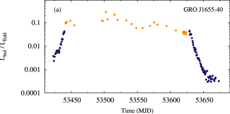
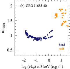
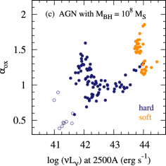
Figure 1: Scaling the GRO J1655-40 outburst to the case of a $10^{8}$M_⊙ black hole in AGN. (a) Lightcurve of GRO J1655-40 with the data used in this paper; hard states - black/blue, soft state - gray/orange. (b)’Stretched’ disc-to-Comptonization index versus the $EF_{E}$ flux at 3 keV, $(ef_{e})_{3}$, for GRO J1655-40 (see Sobolewska, Gierliński, Siemiginowska 2009). (c) Simulated $\alpha_{\rm ox}$ vs. monochromatic luminosity at 2500Å. Open circles indicate the results from simulated AGN SEDs based on the GRO J1655-40 spectra with little or no disc component.

Active galactic nuclei (AGN) are strong sources of optical and X-ray radiation. Their emission is commonly thought to be composed of two main components: thermal blackbody type radiation emerging from a geometrically thin and optically thick accretion disc in the optical/UV band, and a non-thermal power-law type hard X-ray tail believed to be formed by inverse Compton up-scattering of the disc seed photons by energetic electrons in a hot plasma, so called X-ray ’corona’ (e.g. Magdziarz et al. 1998; Chiang 2002; Chiang & Blaes 2003; Sobolewska, Życki & Siemiginowska 2004a,b; Middleton, Done & Gierliński 2007; Vasudevan & Fabian 2009). Dependencies between the X-ray and optical/UV luminosities, and the shape of the spectral energy distribution (SED) in different cosmic times are studied to constrain accretion models, understand AGN variability, AGN influence on intergalactic medium and a contribution to the X-ray background. These dependencies have been investigated by many authors (e.g. Young, Elvis & Risaliti 2010; Grupe et al. 2010; Lusso et al. 2010; Zamorani et al. 1981; Avni & Tananbaum. 1982; Wilkes et al. 1994; Yuan, Siebert & Brinkmann 1998; Bechtold et al. 2003; Vignali, Brandt & Schneider 2003; Strateva et al. 2005; Steffen et al. 2006; Kelly et al. 2007, 2008). Most of the authors agree that the X-ray loudness, defined as

$$\alpha_{\rm ox}=-\frac{\log(\nu\rm L_{\nu})_{o}-\log(\nu\rm L_{\nu})_{x}}{\log\nu_{o}-\log\nu_{x}}+1,$$ (1)

where $(\nu L_{\nu})_{o}$ and $(\nu L_{\nu})_{x}$ are monochromatic luminosities at the rest frame optical/UV and X-ray energies, $\lambda_{o}=c/\nu_{o}=2500$Å and $E_{x}=h\nu_{x}=2$ keV, respectively, correlates primarily with L_ν,o, and that there is a strong correlation between L_ν,o and L_ν,x. The correlation between the rest frame 2–10 keV X-ray photon index, $\Gamma_{x}$, and optical/UV or X-ray luminosities is still a matter of debate, however a correlation of $\Gamma_{x}$ with the Eddington luminosity ratio has been reported by several authors (e.g. Grupe 2004, Kelly et al. 2008, Sobolewska & Papadakis 2009). Kelly et al. (2008) pointed out that this correlation may be induced by the underlying dependence of the X-ray photon index on the mass accretion rate. Grupe (2006) found a mild correlation between the X-ray loudness and the X-ray spectral index, $\alpha_{x}$ = $\Gamma_{x}-1$, but its significance was low. In addition, correlations of $\alpha_{\rm ox}$ and $\Gamma_{x}$ with redshift are studied in attempt to discover how quasars have been evolving over the cosmic time. It seems that quasars’ SEDs become more X-ray quiet for higher redshifts, but no significant intrinsic dependence of $\Gamma_{x}$ on the redshift was found.

Galactic black hole binaries (GBHs) represent another class of accreting black holes. Similarly to AGN, they also accrete matter through an accretion disc emitting thermal X-rays, posses a hard X-ray emitting ’corona’ and may show collimated outflows in the form of jets, or uncollimated outflows, the so called disc winds. GBHs exhibit state transitions that can be followed throughout the entire outburst cycle of the duration of the order of $\sim$100 days. The GBHs state transitions happen on timescales of hours or shorter. Therefore, X-ray spectra of GBHs provide a way to study properties of the disc-corona accretion system at different luminosity levels.

Signatures of AGN outbursts and their different luminosity states have been recently observed in X-rays (for example observations of clusters of galaxies, e.g. Fabian et al. 2001, McNamarra & Nulsen 2007; compact radio sources, e.g. Czerny et al. 2009; and X-ray jets, e.g. Siemiginowska et al. 2007). However, in the case of AGN characteristic transition timescales exceed 10⁵ years, as the timescales are thought to scale inversely with the black hole mass, and so AGN population studies are needed in order to identify sources in different spectral states (e.g. Körding, Jester & Fender 2006). One way to deal with this difficulty is to follow GBHs spectral evolution through different states and then apply its pattern to a population of AGN to identify their states.

The Rossi X-ray Timing Experiment (RXTE) archives contain GBH data that cover many complete X-ray outbursts, during which an object emerges from the quiescence, reaches a significant fraction of Eddington luminosity, and fades away. Application of even simple models to these data leads to a good phenomenological understanding of accretion mechanism at different luminosity levels. Spectral studies accompanied by studies of the high quality X-ray power spectra facilitate classification of GBHs spectral states (e.g. Remillard & McClintock 2006; Done, Gierliński & Kubota 2007).

The situation is quite different in the case of AGN. It is commonly accepted that the typical timescales in accreting black holes are inversely proportional to the black hole mass, and so the timescales of state transitions in AGN are too long to be covered by an observing run. As a consequence, it is unlikely to observe a state transition of an individual AGN. However, a large enough unbiased sample of AGN should contain a mixture of objects in different spectral states. Still, it is not trivial to determine a spectral state of an AGN relying solely on the X-ray power-law like continuum. The Galactic black hole binaries phenomenology clearly shows that a SED with a typical X-ray photon index $\Gamma_{x}\sim 2$ may be representative of a hard, intermediate, or very high spectral state. Even though these GBH states show similar hard X-ray spectra, the properties of their thermal disc components peaking in soft X-rays around 1 keV differ dramatically (e.g. Remillard & McClintock 2006; Done et al. 2007). Since the mass of the accreting black hole affects the characteristic temperature of the accretion disc emission: the disc spectrum of more massive objects shifts towards lower energies. As a result AGN’s discs emerge in the optical/UV band. Confirmed GBHs are homogeneous in terms of the mass of the compact object and they all contain black holes with mass of the order of several Solar masses (see e.g. Done & Gierliński 2003, Remillard & McClintock 2006, and references therein). In contrast, the AGN samples contain black holes that differ in mass by 3–4 orders of magnitude (e.g. Grupe et al. 2010; Merloni et al. 2010; Shen et al. 2008; Kelly et al. 2008). Unfortunately, good quality simultaneous AGN data covering a multiwavelength optical/UV to hard X-ray band are rarely available. Consequently, it is not straightforward to disentangle the intrinsic and apparent (e.g. due to absorption or reflection) AGN X-ray spectral variability and develop an AGN spectral state phenomenology, similar to that of GBHs. The method to assign spectral states to AGN based on their power spectra (see e.g. Uttley & McHardy 2005, Arévalo et al. 2006, McHardy et al. 2007) can be applied only to a few best monitored objects with quality light curves. Clearly, there is a need to develop indirect methods of assigning the accretion mode to the SEDs of AGN.

In Sobolewska, Gierliński, Siemiginowska (2009, hereafter Paper I) we defined the disc-to-power law index for Galactic black hole binaries, $\alpha^{\prime}_{\rm GBH}\simeq 0.32(\alpha_{\rm GBH}-1)+1$, which corresponds to the X-ray loudness parameter, $\alpha_{\rm ox}$, used to characterize the AGN broad-band optical/UV/X-ray spectra. The $\alpha_{\rm GBH}\simeq 0.824\log[(ef_{e})_{\rm 3}/(ef_{e})_{\rm 20}]+1$ (where $ef_{e}$ denotes the $EF_{E}$ flux in erg cm^-2 s^-1) was defined as the index of a nominal power law between the 3 keV, where the accretion disc dominates the spectrum of a GBH (with the exception of the hard state) and 20 keV, where the spectrum is dominated by a power law emission, modelled as Comptonization of the seed disc photons in the hot corona. The $\alpha^{\prime}_{\rm GBH}$ accounts for the many orders on magnitude difference between the energies for which the $\alpha_{\rm GBH}$ and $\alpha_{\rm ox}$ are defined (3-to-20 keV and 2500Å-to-2 keV, respectively). We showed that the distribution of $\alpha^{\prime}_{\rm GBH}$ shows three distinctive peaks around $\sim$1, 1.5 and 2, which correspond to hard, intermediate/very high and soft spectral states, respectively. Hence, $\alpha^{\prime}_{\rm GBH}$ and so $\alpha_{\rm ox}$, together with the X-ray photon index, can be indicators of a spectral state of accreting black holes.

In the present paper we develop the Paper I idea in more detail. We use the GBH phenomenology to simulate an outburst of AGN. We use a physical model of accretion to describe the spectra of a representative GBH, GRO J1655-40, at various luminosity levels, and then we scale the seed photons temperature and bolometric luminosity in the best fitting models with mass, as in the standard Shakura-Sunyaev disc case, to study accretion onto a supermassive black hole. Next, we separate the simulated AGN spectral states in the $\alpha_{\rm ox}$ vs. $(\nu L_{\nu})_{o}$ plane for various classes of AGN, including broad and narrow line Type 1 Seyferts and LINERs. We investigate if the mass spread in the observed AGN samples can contribute to the observed correlation between the X-ray loudness, $\alpha_{\rm ox}$) and monochromatic luminosity at 2500Å.

The structure of the paper is as follows. In Sec. 2 we describe the data selection criteria and data reduction procedure as well as give details of data modeling. Section 3 we present our method of mass scaling of a GBH outburst to the case of AGN. In Sec. 4 we present simulated spectra, resulting correlations between the parameters, and compare our work with observational samples. Finally, in Sec. 5 we discuss and conclude our results.

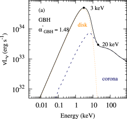
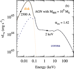
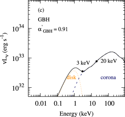
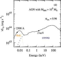
Figure 2: (a/c) A soft/hard state spectrum of GRO J1655-40 (solid/black) formed by a disc blackbody (dotted/orange) and Comptonization (dashed/blue) components. The ’stretched’ disc-to-Comptonization index, $\alpha^{\prime}_{\rm GBH}$, was calculated between 3 and 20 keV. (b/d) A soft/hard state SED of GRO J1655-40 from (a/c) scaled to the case of an AGN hosting a $10^{9}$M_⊙ black hole. The X-ray loudness $\alpha_{\rm ox}$ was calculated between 2500Å and 2 keV.

2 GBH template

2.1 Data selection

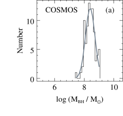
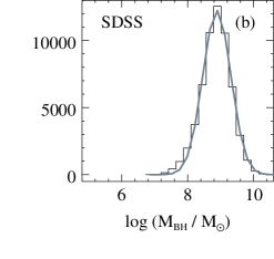
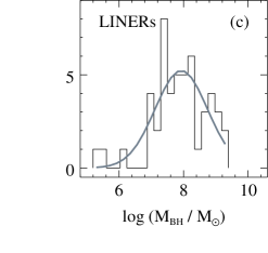
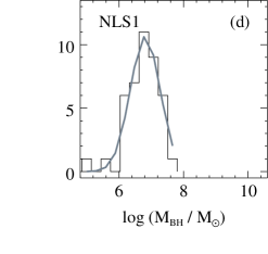
Figure 3: Distributions of AGN black hole masses in different observational samples. (a) COSMOS Type 1 AGN from Merloni et al. (2010), (b)  60.000 SDSS AGN from Shen et al. (2008), (c) compilation of LINERs from Maoz (2007), Gu & Cao (2009) & Eracleous et al. (2010), (d) NLS1s from Grupe et al. (2010). The solid curves are log-normal fits to the distributions with properties listed in Tab. 1.

GBH binaries undergo violent events during which their luminosity may increase by more than 3 orders of magnitude. During these outbursts the sources show variety of different X-ray spectral shapes (e.g. Remillard & McClintock 2006; Done et al. 2006). This spectral variability is relatively well understood (e.g. Gierliński & Done 2004). Typical peak outburst luminosities do not exceed 0.3–0.5$L/L_{E}$ (e.g. Done et al. 2006). This is most probably connected to the physics of the accretion discs that become unstable at high $L/L_{E}$ (e.g. Merloni 2003, Merloni & Nayakshin 2006). A few GBHs sporadically reach the high Eddington ratios (see e.g. references in Done et al. 2006), but only GRS 1915+105 accretes steadily at Eddington ratios $0.3\leq L/L_{E}\leq 3$. It was shown in Done, Wardziński, Gierliński (2004), however, that GRS 1915+105 occupies a different region in their color-color diagram than the ’normal’ GBHs, and it never goes into a ’normal’ hard or soft state.

In our study we are looking for a well monitored outburst of a typical GBH, that would display a variety of different spectral states, and could be easily described with a standard disc+corona model. For these reasons, we have selected the 2005 outburst of a confirmed Galactic X-ray black hole binary GRO J1655–40 hosting a 6.3M_⊙ black hole, located at the distance of 3.2 kpc, with inclination of 30^∘ (Remillard & McClintock 2006). The lightcurve of the outburst is presented in Fig. 1a. The X-ray bolometric luminosity (calculated based on the extrapolated 0.01–1000 keV flux of the best fitting models) changed by more than 3 orders of magnitude, and at the peak of the outburst the system reached $\sim$20–30% of the Eddington luminosity.

In 2005 GRO J1655-40 displayed a variety of GBH spectral states (e.g. Brocksopp et al. 2006; Done et al. 2007), with the spectral variations covering a typical range for its class. This can be seen e.g. in the patterns followed by GRO J1655-40 (Fig. 1b) and other GBHs (Sobolewska et al. 2009) in the $\alpha_{\rm GBH}$ vs. monochromatic luminosity at 3 keV diagrams, and also in the hardness-intensity diagrams presented for other GBHs (e.g. Fender, Belloni & Gallo 2004, Belloni et al. 2005). Hence, we argue that the 2005 data of GRO J1655-40 provide a reasonable SED template to study accretion mechanisms onto a black hole at various luminosity levels. We note, however, that the hard-to-soft state transition in 2005 outburst of GRO J1655-40 happened at $\sim 0.02L/L_{\rm E}$, while it was shown that such a transition may also happen in GBH at much higher ratios, $\geq$0.3$L/L_{E}$ (Gierliński & Newton 2006). Thus our template may lack luminous hard state SEDs, and we discuss its implications later on.

We reduced all data of the 2005 outburst found in the public HEASARC using ftools ver. 6.2. We extracted PCA spectra for detector 2, top layer only and HEXTE spectra from both clusters; one spectrum per pointed observation (see Paper I for the details of data reduction). For modeling we used xspec ver. 11.3 (Arnaud 1996).

2.2 Spectral model

It has been shown (e.g. Gierliński et al. 1999, Done & Gierliński 2003) that the spectral evolution of GBH during an outburst can be explained in terms of variations of the soft photons temperature and hard-to-soft compactness ratio, which depends mostly on the geometry of the disc-corona system. Following these authors, we described the spectra with a sum of the disc blackbody component (diskbb) and Comptonization (eqpair, Coppi 1999). The eqpair code gives the ratio between the power in seed photons, $\ell_{s}$ and hot electrons, $\ell_{h}$. This ratio, $\ell_{h}/\ell_{s}$, depends mostly on the geometry of the accretion flow and defines the spectral shape of the hard X-ray continuum. Typically, the hard state is characterized by $\ell_{h}/\ell_{s}\gg 1$, (ultra) soft state by $\ell_{h}/\ell_{s}\ll 1$ and very high/intermediate state by $\ell_{h}/\ell_{s}\sim 1$. The other important model parameters include the optical depth, $\tau$, the temperature of the seed photons, $kT_{s}$, and the ratio of the nonthermal-to-thermal compactness $\ell_{nth}/\ell_{th}$. The index of the injected non-thermal electrons was fixed at $\Gamma_{\rm inj}=2.5$ in all but 14 cases for which the fits resulted in $1<\Gamma_{\rm inj}<3$. The model is not very sensitive to the changes of the total compactness $\ell_{tot}=\ell_{h}+\ell_{s}$. The eqpair also accounts for a reflection of the hard X-rays from a cold medium (presumably an accretion disc). This reflected component is parametrized by the reflection amplitude and ionization parameter. The complete model used in XSPEC was defined as constant*wabs(diskbb+eqpair), where constant allows for normalization between PCA and HEXTE data and wabs models the Galactic absorption with $N_{H}$ fixed at 0.8$\times 10^{22}$cm^-2 (Done & Gierliński 2003, and references therein). The eqpair model is particularly well suited for our study because it allowes for straight forward scaling of the spectra between the accreting black holes of different mass by applying due corrections to the seed photons temperature, while keeping the geometry of accretion constant.

We modeled 94 hard state spectra of the outburst and 38 representative soft state spectra; 132 data sets in total. The times of the data sets that we used are indicated in Fig. 1a. We set a lower limit of 0.4 keV on the disc photons temperature, $kT_{bb}$, and in the case of the hard state spectra we fix $kT_{bb}$ at 0.4 keV. Fits to 119 data sets (90%) result in the null hypothesis probability, $p_{\rm null}$, greater than 5%. The remaining 13 data sets with $p_{\rm null}>5$% show residuals around 6–7 keV which are reminiscent of an iron line emission, which is not computed together with the reflected component by the eqpair code. Thus in these 13 cases we include explicitly the relativistic line model of Laor (1991), laor. We fix the emissivity of the line at 3, and the inner and outer radius at the values used to compute the reflected component in eqpair: 20 and 1000 gravitational radii, respectively. After addition of the line, the fits to 9 of 13 data sets resulted in $p_{\rm null}>5$%.

We notice that it has been reported by e.g. Sala et al. (2007) and Miller et al. (2008) that XMM-Newton and Chandra spectra of GRO J1655-40, respectively, show features implying strong accretion disc winds. A number of absorption lines in the 7–9 keV band have been observed. However, RXTE has a much poorer energy resolution than Chandra or XMM-Newton, and so we are not able to handle properly these absorption features.

Nevertheless, we conclude that we have found a model that fits well 128 of 132 considered data sets, which means that the model fits our set of data well from the statistical point of view (see e.g. Sobolewska & Papadakis 2009). An example of soft/hard state models fitted to the GRO J1655-40 data is shown in Figs. 2a/c.

Following Paper I, we calculate the disc-to-Comptonization index, $\alpha^{\prime}_{\rm GBH}$, for GRO J1655-40 based on the best fitting spectral models. The diagram of $\alpha^{\prime}_{\rm GBH}$ versus the $(ef_{e})_{3}$ flux in keV cm^-2 s^-1 at 3 keV is presented in Fig. 1b, and the hard/soft spectral states that GRO J1655-40 entered during its evolution are indicated with different colors. The values of $\alpha^{\prime}_{\rm GBH}$ for GRO J1655-40 range between 1 and 2, which is in general true also in the case of other GBH (see Paper I), and in the case of AGN’s $\alpha_{\rm ox}$.

3 Method

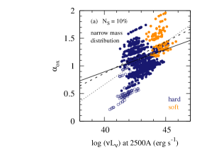
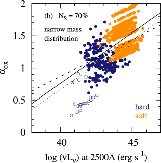
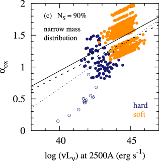
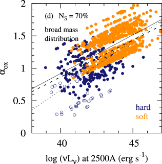
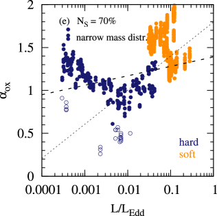
Figure 4: Simulated X-ray loudness as a function of simulated monochromatic luminosity at 2500Å (a–d) and Eddington luminosity ratio (e). The black hole mass was drawn from the distribution in Fig. 3a (a–c,e) and 3c (d). The number of the soft state AGN was assumed to be $N_{S}=70$% in (b,d–e), 10% (a) or 90% (c), hard states - black/blue, soft state - gray/orange, hard state with insignificant disc component - open circles. From comparison of panels (b) and (d) it can be seen that for a narrow FWHM of the AGN mass distribution, the simulated AGN spectral are well separated, and they overlap when the FWHM increases. The solid lines represent the best fits to the simulations, while the dotted and dashed lines are the best fits to the observational samples of Lusso et al. (2010; 545 X-ray selected type 1 AGN, from the XMM-COSMOS) and Grupe et al. (2010; 92 bright soft X-ray selected AGN observed with Swift), respectively. The hard state simulations indicated with the open circles where neglected during the fit because very low level of the disc component would make such AGN spectra difficult to recognize in real data. The slope of the simulated correlation depends on the assumed number of the soft state AGN in the sample. (e) A change of the sign of the $\alpha_{ox}$ vs. $L/L_{E}$ correlation can be observed for $L/L_{\rm E}\approx 0.01$. This result does not depend on the adopted AGN mass distribution. The dotted and dashed lines correspond to the correlations found by Lusso et al. (2010) and Grupe et al. (2010), respectively.

We simulate spectra of AGN by scaling the disc temperature and the bolometric luminosity of our collection of the best-fitting GRO J1655–40 models. For a standard Shakura-Sunyaev geometrically thin optically thick accretion disc, the disc temperature scales with the black hole mass as $T_{\rm disc}\propto M^{-1/4}$, and the bolometric luminosity is proportional to the black hole mass, $L_{\rm bol}\propto M$. We assume that the accretion flow geometry, and hence the heating to cooling compactness ratio, $\ell_{h}/\ell_{s}$, varies in the same way as the function of the mass accretion rate both in Galactic and supermassive black holes. We set the normalization of the iron line, when present in the baseline spectrum, to zero, since it does not contribute significantly to the total simulated AGN flux. Our goal is to check if taking into account the mass distribution among the AGN samples can provide insights to the origins of the observed dependence between the X-ray loudness, $\alpha_{\rm ox}$) and optical/UV luminosity at 2500Å.

3.1 Masses of AGN

For our study we select the AGN samples with measured black hole mass. Black hole mass measurements in AGN are not trivial. However, various methods (e.g. reverberation mapping and correlations with the widths of emission lines) resulted in black hole mass estimates ranging between 10⁶ and 10¹⁰ Solar masses. Figure 3 shows mass distributions for samples of AGN compiled from the literature.

Table 1: Properties of lognormal mass distributions in different AGN samples from literature.

Sample	#of AGN	$<\log\frac{{\rm M}_{\rm BH}}{{\rm M}_{\odot}}>$	FWHM	Ref.
T1 COSMOS	86	8.40	0.75	[1]
T1 SDSS	$\sim$60.000	8.89	1.00	[2]
LINERs	50	7.9	1.9	[3–5]
NLS1	42	6.8	1.1	[6]

[1] Merloni et al. (2010), [2] Shen et al. (2008), [3] Maoz (2007), [4] Gu & Cao (2009), [5] Eracleous, Hwang & Flohic (2010), [6] Grupe et al. (2010).

In Fig. 3a we show the mass distribution reported for 86 Type 1 Broad Line AGN by Merloni et al. (2010) as part of the COSMOS project. The masses were consistently calculated based on the MgII emission line, however the sample spans relatively narrow ranges of redshifts ($1<z<2.2$) and luminosities ($44.5<\log L_{\rm bol}<46.5$). For comparison, in Fig. 3b we show the results of Shen et al. (2008), for Type 1 Broad Line AGN in SDSS. This sample contains $\sim$60.000 objects with redshifts and luminosities in the $0.1<z<4.5$ and $44.5<\log L_{\rm bol}<48$ range, with masses calculated based on MgII, CIV or H_β lines. This is the largest AGN sample with black hole mass measurements. However, the authors point out that the estimations based on the CIV line may be biased due to the line being disc wind dominated.

In addition to the Type 1 Broad Line AGN, we consider a sample of LINER galaxies. Black hole mass measurements are challenging because of the host galaxy domination in the optical band. We compile a LINERs sample galaxies from Maoz (2007), Gu & Cao (2009) and Eracleous et al. (2010) containing black hole mass estimates for 50 sources. The estimated Eddington ratios for LINERs (e.g. Gu & Cao 2009, Eracleous et al. 2010) indicate that they accrete at low rates and thus may be the counterparts of the hard state GBHs. We test this possibility in Sec. 4.2.

Finally, we consider Narrow Line Seyfert 1 galaxies (NLS1). We study a NLS1 subsample from Grupe et al. (2010) defined as FWHM(H${}_{\beta})<2000$ km s^-1 (Osterbrock & Pogge, 1985; Goodrich 1989). These objects have reliable estimates of the accretion rates based on the simultaneous SEDs in optical and X-ray bands. NLS1 are believed to have higher Eddington ratios (and lighter black holes) than their broad line counterparts. In Sec. 4.2 we study if they can be considered as counterparts of the soft state GBHs.

Distribution of AGN masses in all the above samples can be satisfactorily described by a lognormal functions with means and FWHMs listed in Table 1. Thus, in this paper we will assume that the masses of black holes in AGN have a lognormal distribution. The means of the above distributions are different: $\log({\rm M}_{\rm BH}/{\rm M}_{\odot})=6.8$ and 8.9 for NLS1s and SDSS samples, respectively. The FWHMs vary between 0.75 and 1.9 for the COSMOS and LINERs samples, respectively. We will study the effect of a narrow vs. broad mass distribution in our simulations.

3.2 Spectral states of AGN

Based on the modelling of the GRO J1655-40 spectra we conclude that this source was in a soft spectral state for $t_{s}\sim 0.7{\rm T}$, and in a hard spectral state for $t_{h}\sim 0.3{\rm T}$ of the 2005 outburst (where T is the total time of the outburst). The situation in any real unbiased AGN sample would be different in the sense that in the case of GRO J1655-40 we have many spectra of the same source in various spectral states, while in a real AGN sample we would record usually one spectrum for each AGN. However, a large AGN sample would contain a mixture of hard and soft state SEDs, with a fraction of the soft state SEDs, $N_{S}/N$ (where $N_{S}$ and $N$ are the number of the soft AGN SEDs and the total number of AGN SEDs, respectively), corresponding to $t_{s}/{\rm T}$ in a typical GBH outburst.

The duration of the time spend in either state differs for different GBHs (see e.g. Figs. 4–5 in Done et al. 2007), and depends most probably on a number of physical parameters. It is not clear what would be the expected ratio of the hard to soft state AGN (or GBH) spectra in a large sample. Thus, we first assume that $N_{S}/N=0.7$ (corresponding to the $t_{s}/{\rm T}$ ratio in the 2005 outburst of GRO J1655-40), and then we check how our results change if we assume that $N_{S}/N=0.1$ and 0.9.

To assign a spectral state to the simulated AGN spectrum we draw a number from a uniform distribution between 0 and 1. If this number is between 0 and $N_{S}/N$, we assign a soft spectral state to the AGN spectrum that will be simulated. Otherwise the AGN spectrum is simulated assuming that the spectral state is hard.

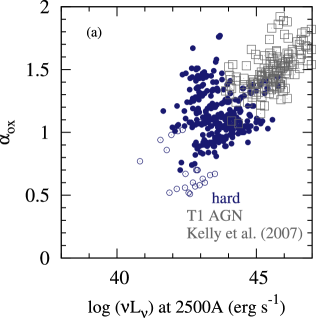
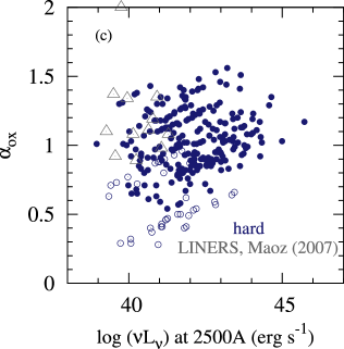
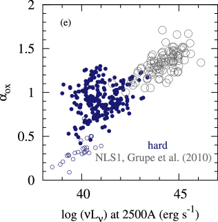
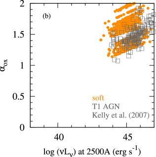
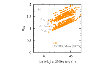
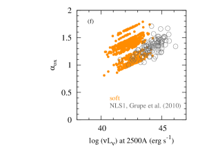
Figure 5: Comparison of properties of the simulated AGN spectra with observational samples, hard states - black/blue, soft state - gray/orange, hard state with insignificant disc component - open circles. (a-b) Kelly et al. (2008) Type 1 AGN, (c-d) Maoz (2007) LINERs, (e-f) NLS1 from Grupe et al. (2010) superimposed on the simulated hard and soft state AGN data (with $\log$ of AGN mass drawn from a Gaussian distribution as in Figs. 3a, 3c and 3d, respectively). Observed LINERs overlap with the hard state simulated AGN, while observed Type 1 quasars and NLS1s overlap with the simulated soft state AGN.

3.3 Simulating the AGN SEDs

After determining the simulated AGN spectral state, we randomly choose a spectrum from the 94 hard or 38 soft state observations of GRO J1655-40 to access the mass accretion rate and spectral parameters that we assume to be constant between the original GBH and simulated AGN spectra, and independent on the mass of the accreting black hole: the $\ell_{h}/\ell_{s}$ compactness ratio, the optical depth of the Comptonizing corona, the seed photons Compactness, and the thermal/non-thermal electron fraction in the corona. Next, we randomly draw a black hole mass from an observationally motivated lognormal distribution, and scale the disc temperature and luminosity in the original GBH spectrum with the mass. We repeat the entire procedure $N=1000$ times to get a large enough simulated sample of AGN spectra for comparison with the observational data. As an example, in Fig. 2b/d we plot a simulated soft/hard state AGN spectrum which was obtained by scaling a soft/hard state GBH spectrum (Fig. 2a/c) assuming that the AGN hosts a 10⁹M_⊙ black hole.

4 Results

We calculate $\alpha_{\rm ox}$ for each simulated AGN spectrum and we plot it as a function of the simulated monochromatic luminosity at 2500Å. The observed correlation is clearly present in the simulated data. Initially, we investigate the effect of the width of the black hole mass distribution on the simulated $\alpha_{ox}$ vs. $\nu L_{\nu}$ at 2500Å correlation.

First we perform our simulations for the log-normal AGN mass distribution as in Merloni et al. (2010, Fig. 3a), with the narrowest FWHM=0.75 among the four distributions in Fig. 3. We assume that $N_{S}=70$% of the simulated AGN are in a soft spectral state. The results are presented in Fig. 4b. Indeed, observationally motivated log-normal mass distribution in this sample leads to a correlation between the $\alpha_{\rm ox}$ and monochromatic optical/UV luminosity at 2500Å. The hard and soft simulated states are well separated.

Next, we repeat our simulations using the lognormal mass distribution resulting from fitting the combined Maoz (2007), Gu & Cao (2009) and Eracleous et al. (2010) LINERs masses (Fig. 3c). This distribution has FWHM=1.9, the broadest among the four samples in Fig. 3. It can be seen in Fig. 4d that for LINERs the hard and soft states overlap for $\sim$5 orders of magnitude in $(\nu L_{\nu})_{o}$. Based on this we conclude that the larger the width of the distribution used to draw the AGN black hole masses, the more significant the spread of the simulated quantities, and the more pronounced the overlap of the hard and soft spectral states.

4.1 Correlation analysis

We quantify the simulated $\alpha_{\rm ox}$ vs. $(\nu L_{\nu})_{o}$ correlations by fitting the simulated data with a function of the following form: $\alpha_{\rm ox}=a\times\log(\nu L_{\nu})_{o}+b$.

During the fit we neglect the hard state data indicated with open circles which where simulated based on the GRO J1655-40 observations with the disc flux lower than $F_{d}=5\times 10^{-11}$ erg s^-1 cm^-2. Among the 94 considered GRO J1655-40 hard state observations there were 11 datasets that were well described by the Comptonized continuum with a flux $F_{c}$ dominating significantly over the disc flux $F_{d}$ in the total spectrum. A case of an AGN with similar geometry (i.e. extremely low disc flux) would be difficult to detect in optical/UV due to the emission of a host galaxy that would dominate in this band. However, such an AGN would still be detected in the X-ray band with an X-ray SED resembling a power law.

Our fits result in

$$\alpha_{ox}^{\rm COSM,70}=(0.157\pm 0.008)\times\log(\nu L_{\nu})_{o}-(5.5\pm 0.4)$$

$$\alpha_{ox}^{\rm SDSS,70}=(0.161\pm 0.008)\times\log(\nu L_{\nu})_{o}-(5.8\pm 0.4)$$

$$\alpha_{ox}^{\rm LINER,70}=(0.119\pm 0.005)\times\log(\nu L_{\nu})_{o}-(3.8\pm 0.2)$$ (2)

$$\alpha_{ox}^{\rm NLS1,70}=(0.125\pm 0.008)\times\log(\nu L_{\nu})_{o}-(4.1\pm 0.3)$$

for AGN SED sets simulated based on all four AGN mass distributions from Fig. 3, respectively. The range of slopes we find in this correlation is consistent with that seen in real data. For example, Grupe et al. (2010) found a slope of 0.114$\pm$0.014 based on the study of 92 bright soft X-ray selected AGN observed with Swift (a combination of narrow line and broad line Seyfert 1s), while Lusso et al. (2010) reported a slope of 0.154$\pm$0.010 in the XMM-COSMOS sample of 545 X-ray selected type 1 AGN. Their correlations are indicated in Fig. 4 with dotted and dashed lines, respectively. The best fits to the SEDs simulated using narrow (COSMOS) and broad (LINERs) mass distributions are indicated with solid lines in Figs. 4a–d.

The fitted slopes depend on the assumed number of the soft state spectra in the AGN sample. Figures 4a and 4c show how the correlation changes if we assume that $N_{S}=10$% or 90% of the AGN, respectively, are in a soft state, for the case of a narrow mass distribution from Fig. 3a. For the four considered AGN mass distributions we obtained $a^{10}=0.078$–0.85 for $N_{S}=10$% and $a^{90}=0.107$–0.121 for $N_{S}=90$%.

Additionally, we check if the simulated AGN’s $\alpha_{\rm ox}$ is related to the bolometric luminosity in Eddington units. In Fig. 4e we plot $\alpha_{ox}$ vs. $L/L_{E}$ for a narrow mass distribution (Fig. 3a), assuming $N_{S}=70$%. Interestingly, the simulated X-ray loudness correlates positively with the Eddington ratio down to approximately $\lambda_{\rm crit}\approx 0.01$ $L/L_{\rm E}$ and below this value the correlation changes its sign. In Fig. 4c we superimpose our simulations and the correlations found in real data by Lusso et al. (2010) and Grupe et al. (2010) (dotted and dashed lines, respectively). The correlation reported by Lusso et al. matches the slope produced by our simulated SEDs down to the critical Eddington ratio, $\lambda_{\rm crit}$. These results do not depend either on the properties of the adopted mass distribution or on $N_{S}$.

4.2 Spectral states of AGN

We compare our simulated data with the known AGN samples, which have measurements of both the monochromatic luminosity at 2500Å and $\alpha_{\rm ox}$, and preferably also the black hole estimates. We assume in this section that $N_{S}=70$%, but we stress that the results do not depend on this parameter.

Neither Merloni et al. (2010) nor Shen et al. (2008) have X-ray observations for their complete samples. For that reason, first we consider the broad line AGN (a SDSS subsample) from Kelly et al. (2007). We compare them with the simulated data resulting from hard (black/blue) and soft (gray/orange) state spectra of GRO J1655-40 scaled to the case of AGN, using the Shen et al. (2008) mass distribution. We use the Shen et al. distribution (not the Merloni et al. one) because it has the mean and FWHM close to those of the Kelly et al. sample. In Figs. 5a–b we superimpose the simulated and observed data. It can be seen that the observations do not overlap with the simulated hard state AGN spectra, while they do occupy the same region in the plot as the simulated soft state AGN spectra.

The interpretation of the spectral states of LINERs (Figs. 5c–d) appears more complex since the data points derived from the real SEDs (Maoz 2007) overlap both with the hard and soft points (simulated based on the LINERs mass distribution, Fig. 3c). However, it can be seen in Fig. 6 that in the case of the simulated soft state AGN, the SEDs that result in $\log(\nu L_{\nu})_{o}\approx 39.5$–41.3 (as reported by Maoz 2007) require low black hole masses, M/M${}_{\odot}<10^{6}$, whereas in the case of simulated hard state AGN, the SEDs require black hole masses of M/M${}_{\odot}\sim 10^{6}$–10⁸ to reach comparable $\log(\nu L_{\nu})$ at 2500Å. Since the LINERs in Maoz (2007) have rather high masses (as indicated with the gray rectangles in Fig. 6) we conclude that most probably these objects are in a hard spectral state.

In Figs. 5e–f we perform similar comparison for a subsample of NLS1 from Grupe et al. (2010). We use the values of $\alpha_{\rm ox}$ provided by the authors in Table 5, column 6, to calculate the monochromatic luminosity at 2500Å from tabulated values of the UV slope, $\alpha_{\rm UV}$, and luminosity at 5100Å (columns 5 and 13, respectively). We compare the observations with the simulations for the mass distribution of the same sample (Fig. 3d). Similarly as in the case of broad line AGN of Kelly et al., the NLS1s in the sample of Grupe et al. do not overlap with the hard state simulated SEDs, while they do overlap with the simulated AGN in the soft state.

5 Discussion

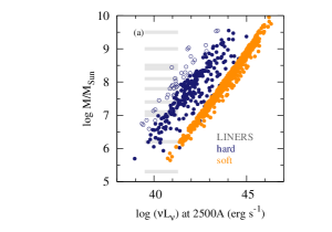
Figure 6: Relation between the mass of the black hole in an AGN and the simulated monochromatic luminosity at 2500Å for mass distribution of LINERS and Type 1 AGN (see Fig. 3c), hard states - black/blue, soft state - gray/orange, hard state with insignificant disc component - open circles. The gray rectangles illustrate masses and the range of $\log(\nu L_{\nu})$ at 2500Å for the real LINERs from Maoz (2007).

We studied the scenario in which the main difference between the GBH and AGN nuclear emission follows from the difference between the masses of the accreting black holes. We assumed that the geometry of the accretion flow characterized by the ratio of the heating and cooling compactnesses, $\ell_{h}/\ell_{s}$, stays the same for both AGN and GBHs in a given spectral state. With these assumptions, we used the RXTE archival data of the 2005 outburst of GRO J1655-40, a well studied GBH, to simulate an outburst of an AGN hosting a 10⁹M_⊙ black hole. Based on the simulated AGN spectra, we calculated $\alpha_{\rm ox}$, the simulated X-ray loudness, and $(\nu L_{\nu})_{o}$, the monochromatic luminosity at 2500Å. We studied how these two parameters would behave during a hypothetical AGN outburst.

Next, we considered a relation between the simulated $\alpha_{\rm ox}$ and $(\nu L_{\nu})_{o}$ in a sample of AGN with a range of masses. We simulated the AGN’s SEDs for a sample of 1000 AGN with masses randomly drawn from a log-normal distribution. The mass distributions were observationally motivated. We considered different classes of AGN: broad line AGN, narrow line Seyfert 1s and LINERs.

Our results suggest that in a sample of AGN with a narrow range of black hole masses one should expect a deviation from a simple correlation between $\alpha_{\rm ox}$ vs. $(\nu L_{\nu})_{o}$. Instead, a characteristic U-shape would be displayed. In a sample of AGN with a broad range of black hole masses, the $\alpha_{\rm ox}$ vs. $(\nu L_{\nu})_{o}$ correlation appears naturally as the result of the mass spread. The slope of the correlations that we derive from the simulated SEDs depends on the assumed number of the soft states in the sample, $N_{S}$, and is consistent with those observed in real SEDs (e.g Grupe et al. 2010, Lusso et al. 2010, and references therein) for $N_{S}\geq 70$%.

We also studied the relation between the simulated $\alpha_{\rm ox}$ and the Eddington luminosity ratio, $L/L_{\rm E}$. We found that the X-ray loudness correlates with the luminosity in Eddington units down to $\lambda_{\rm crit}=L_{\rm crit}/L_{\rm E}\approx 0.01$, and the slope of this correlation roughly matches that reported by Lusso et al. (2010). This result does not depend either on the adopted AGN mass distribution or on the $N_{S}$. The correlation down to $\lambda_{\rm crit}$ is formed by both, soft and hard state simulated SEDs. Below $\lambda_{\rm crit}$ we find only the hard state simulated SEDs, and the correlation changes its sign. This has not been observed yet mainly due to the difficulties in determining $\alpha_{\rm ox}$ in low luminosity AGN with optical spectra often dominated by the host galaxy. Our result provides thus a prediction for future observational studies. Interestingly, in a study of X-ray bright optically normal galaxies (XBONGs) Civano et al. (2005) found that the broad band IR-opt/UV-Xray SEDs of two of their objects can be explained with the Elvis et al. (1994) radio quiet template, that is characterized by $\alpha_{\rm ox}=1.38$. The accretion rate of these two XBONGs was estimated at 0.001$L/L_{\rm E}$, and hence they would fit on the branch of our simulated $\alpha_{ox}$ vs. $L/L_{\rm E}$ correlation with a negative slope, confirming our prediction that the correlation changes its sign below $\lambda_{\rm crit}$. Even more intriguingly, the critical value $\lambda_{\rm crit}\approx 0.01$ matches that for which a change in the sign in the correlation between the X-ray photon index, $\Gamma_{x}$, and Eddington luminosity ratio was reported for AGN (e.g. Green et al. 2009) and GBHs (Wu & Gu 2008, Sobolewska et al. in preparation).

Finally, we investigated a possibility of determining the spectral states of AGN by comparing the simulated data with the observational data of bright Type 1 AGN, NLS1s and and LINERs. We found that the LINERs are most probably the counterparts of the GBH hard state SEDs, while the bright Type 1 AGN and NLS1s overlap with the regions occupied by the simulated soft state SEDs in the $\alpha_{\rm ox}$ vs. $\nu L_{\nu}$ diagram.

It can be noticed in Fig. 5f that the NLS1 luminosities reach $\log(\nu L_{\nu})_{o}\simeq 46$ while the simulations do not exceed $\log(\nu L_{\nu})_{o}\simeq 44.5$, even though we use the same sample to determine the mass distribution for simulations and to compare the simulations with observations. This difference in luminosity may indicate that the brightest NLS1s exceed the maximum $L/L_{\rm E}$ in our GRO J1655-40 template by $\sim 1.5$ order of magnitude, which would push the Eddington ratios of NLS1s to the super Eddington regime of up to 6$L/L_{\rm E}$. Indeed, Grupe et al. (2010) estimated that in 31 of 43 objects in their NLS1 sample the Eddington ratio exceeds the peak luminosity of GRO J1655-40 in Eddington units (17 of them are super Eddington, with the highest estimate of the Eddington ratio being $\sim 13L/L_{\rm E}$).

Typical GBHs rarely exceed $0.3L/L_{\rm E}$ (e.g. Done et al. 2007). The only example of a GBH showing a steady accretion flow at high Eddington fraction is GRS 1915+105 (e.g. Done et al. 2004) that can reach 3 times the Eddington limit. However, at high $L/L_{\rm E}$ the GBH accretion is most probably influenced by powerful wind and jet outflows (e.g Janiuk, Czerny & Siemiginowska 2002, Neilsen & Lee 2009). Also, at high $L/L_{\rm E}$ the standard Shakura-Sunyaev disc becomes unstable and a different, possibly advection dominated optically thick, solution may be more appropriate to describe such SEDs (Abramowicz et al. 1988). They may not be easily scalable between GBHs and AGN and are beyond the scope of the present paper.

Gierliński & Newton (2006) described two types of the hard-to-soft state transition in GBHs. They differ in terms of the time needed to change between the states and the Eddington ratios at which the transition is triggered. The hard-to-soft state transition in the 2005 outburst of GRO J1655-40 would belong to the dark/fast (DF) category with $L/L_{E}\simeq 0.02$ at the beginning of the transition. That means that our template may lack luminous hard state SEDs. GX 339-4 outburst in 2002/2003 can be an example of a bright/slow (BS) transition with $L/L_{E}\simeq 0.2$ when the transition started (Fender et al. 2004, Gierliński & Newton 2006, although notice the uncertainty of GX 339-4 black hole mass estimates, e.g. Hynes et al. 2004, Zdziarski et al. 2004, Munoz-Darias, Cesares & Martinez-Pais 2008). The hardness-intensity diagrams for GX 339-4 show that the low state intensity increases before the transition while the hardness stays approximately constant. It means that if we included such luminous low state spectra in our template, in the simulated data we would have obtained additional points at $\alpha_{ox}\simeq 1$ (constant hardness and hence constant spectral shape) and $\nu L_{\nu}$ at 2500Å by up to an order of magnitude higher than at present. Hence, this would not change our conclusions about the spectral states of NLS1 and Type 1 AGN because these additional hard state simulated points would appear much below the observed data in both cases (see Fig. 5a,c).

The analogy between the GBHs and AGN was studied also by other authors in the context of determining AGN ’states’. For example, Körding et al. (2006) compared the broad band radio-to-X-ray spectra of GBHs and AGN to study AGN radio states. A number of authors (e.g. Uttley & McHardy 2005, Arévalo et al. 2006, McHardy et al. 2007) investigated methods based on time variability. They noticed similarities in the shape of the power density spectra of GBHs and AGN, which provide an interesting tool in determining the spectral state, but only for a few AGN with good quality long-term lightcurves.

5.1 Low/hard state accretion disc in GBHs

We note that in the hard state the disc of GBHs is cool enough to be shifted away from the RXTE bandpass. GBHs in the hard state have been observed by modern telescopes with a better low energy coverage than that of RXTE: Chandra, XMM-Newton, Suzaku and Swift (see e.g. Miller et al. 2002, Reis et al. 2010). These observations revealed a soft excess reminiscent of an accretion disc with the temperature of $\sim 0.2$ keV extending close to the last stable orbit. If such soft excess is indeed present in the hard state GBH spectra and if it corresponds to a cool accretion disc, our parametrization may not be accurate. As a result our values of $\alpha^{\prime}_{\rm GBH}$ parameter in the hard state may be underestimated since the SED at 3 keV will be dominated by the hard X-rays and not by the disc emission.

GRO J1655-40 in the hard state was observed by XMM-Newton during the 2005 outburst (Obs ID 0112921301). This observation was taken $\sim$4.5 hours after the 90428-01-01-03 RXTE observation. We model these two observations jointly to quantify the effect of the drop in the disc temperature and the shift of the disc component out of RXTE bandpass.

We apply the spectral model described in Sec. 2 to the joint RXTE and XMM-Newton data. We obtain a good agreement of data (0.3–200 keV band) and model, with $\chi^{2}=1089$ for $1081$ degrees of freedom. The temperature of the soft photons converged to kT${}_{\rm bb}=0.166^{+0.011}_{-0.003}$ keV (intermediate between the values reported by Reis et al. 2010 and Díaz Trigo et al. 2007), while we kept it fixed at 0.4 keV in the case of the RXTE fit. The joint fit resulted in the hard-to-soft compactness ratio of $\ell_{h}/\ell_{s}=18.0^{+0.8}_{-1.4}$, higher than in the case of modeling only the RXTE data ($\ell_{h}/\ell_{s}=11.8^{+0.6}_{-1.8}$). We were able to put an upper limit on the optical depth of the corona, $\tau<1.5$ ($\tau<1.0$ for RXTE data only). The Eddington luminosity ratio was $L_{\rm bol}/L_{\rm E}=7.3\times 10^{-3}$ ($6.3\times 10^{-3}$ calculated based on the best fit model to RXTE data only).

The two models, fitted to the RXTE and RXTE+XMM data, scaled to the case of an AGN with 10⁸ M_⊙ gave $\alpha_{\rm ox}=0.82$ and 1.06, respectively. Thus, in the hard state spectra it is possible that we underestimate the simulated $\alpha_{\rm ox}$ by $\sim$25%, at least in the spectra similar to the one described above, with the Eddington luminosity ratio lower than 1%. This would however only strengthen the conclusion followed from Fig. 4e that the $\alpha_{\rm ox}$ vs. Eddington luminosity ratio correlation is expected to change its sign.

Nevertheless, more robust constraints on the temperature of the accretion disc in the hard state GBHs are crucial for the understanding of the spectral evolution of the accreting black holes.

6 Conclusions

• We assumed that the main difference between the radiation processes in the AGN and GBHs is induced by the difference in the black hole mass. We scaled an outburst of a Galactic black hole X-ray binary using an observationally motivated log-normal AGN mass distribution, and we were able to reconstruct the $\alpha_{\rm ox}$ vs. luminosity at 2500Å correlation observed in AGN.

• In a sample of AGN with a narrow range of masses we expect a deviation from the $\alpha_{\rm ox}$ vs. luminosity at 2500Å correlation.

• We predict that the $\alpha_{\rm ox}$ vs. Eddington luminosity ratio correlation changes its sign for Eddington accretion rates below 1%. The XBONGs may be examples of AGN that form the low luminosity branch of the correlation.

• Our study suggest that bright Type 1 quasars and NLS1 are in a spectral state similar to the soft state of GBHs, while LINERS may correspond to the hard state of GBHs.

• Tighter constraints on the behaviour of the accretion disc in the hard spectral state in GBHs are needed in order to understand the balance between the thermal disc emission and the non-thermal Comptonized power-law like hard X-ray emission.

References

- [Abramowicz et al.(1988)] Abramowicz M. A., Czerny B., Lasota J. P., Szuszkiewicz E., 1988, ApJ, 332, 646
- [Arévalo et al.(2006)] Arévalo P., Papadakis I. E., Uttley P., McHardy I. M., Brinkmann W., 2006, MNRAS, 372, 401
- [] Arnaud K. A., 1996, Astronomical Data Analysis Software and Systems V, 101, 17
- [Avni & Tananbaum(1982)] Avni Y., Tananbaum H., 1982, ApJL, 262, L17
- [Bechtold et al.(2003)] Bechtold J. et al., 2003, ApJ, 588, 119
- [Belloni et al.(2005)] Belloni T., Homan J., Casella P., van der Klis M., Nespoli E., Lewin W. H. G., Miller J. M., Méndez M., 2005, A&A, 440, 207
- [Brocksopp et al.(2006)] Brocksopp C. et al., 2006, MNRAS, 365, 1203
- [Chiang(2002)] Chiang J., 2002, ApJ, 572, 79
- [Chiang & Blaes(2003)] Chiang J., Blaes O., 2003, ApJ, 586, 97
- [Civano et al.(2007)] Civano F. et al., 2007, A&A, 476, 1223
- [] Coppi P.S., 1999, in Poutanen J., Svensson R., eds, ASP Conf. Ser. Vol.161, High Energy Processes in Accreting Black Holes. Astron. Soc. Pac., San Francisco, p. 375
- [Czerny et al.(2009)] Czerny B., Siemiginowska A., Janiuk A., Nikiel-Wroczyński B., Stawarz Ł., 2009, ApJ, 698, 840
- [Díaz Trigo et al.(2007)] Díaz Trigo M., Parmar A. N., Miller J., Kuulkers E., Caballero-García M. D., 2007, A&A, 462, 657
- [Done & Gierliński(2003)] Done C., Gierliński M., 2003, MNRAS, 342, 1041
- [Done et al.(2004)] Done C., Wardziński G., Gierliński M., 2004, MNRAS, 349, 393
- [Done et al.(2007)] Done C., Gierliński M., Kubota A., 2007, A&AR, 15, 1
- [Eracleous et al.(2010)] Eracleous M., Hwang J. A., Flohic H. M. L. G., 2010, ApJS, 187, 135
- [Fender et al.(2004)] Fender R. P., Belloni T. M., Gallo E., 2004, MNRAS, 355, 1105
- [Gierliński et al.(1999)] Gierliński M., Zdziarski A. A., Poutanen J., Coppi P. S., Ebisawa K., Johnson W. N., 1999, MNRAS, 309, 496