A Model of Electrowetting, Reversed Electrowetting and Contact Angle Saturation

Abstract

While electrowetting has many applications, it is limited at large voltages by contact angle saturation — a phenomenon that is still not well understood. We propose a generalized approach for electrowetting that, among other results, can shed new light on contact angle saturation. The model assumes the existence of a minimum (with respect to the contact angle) in the electric energy and accounts for a quadratic voltage dependence $\sim U^{2}$ in the low-voltage limit, compatible with the Young-Lippmann formula, and a $\sim U^{-2}$ saturation at the high-voltage limit. Another prediction is the surprising possibility of a reversed electrowetting regime, in which the contact angle increases with applied voltage. By explicitly taking into account the effect of the counter-electrode, our model is shown to be applicable to several AC and DC experimental electrowetting-on-dielectric (EWOD) setups. Several features seen in experiments compare favorably with our results. Furthermore, the AC frequency dependence of EWOD agrees quantitatively with our predictions. Our numerical results are complemented with simple analytical expressions for the saturation angle in two practical limits.

I Introduction

The term Electrowetting, in its broadest sense, refers to techniques by which one can control the apparent wettability (characterized by the contact angle) of liquids, by applying an external electric potential Mimmena_1980 ; Beni_1980 ; Gorman_1995 ; Sondag-Huethorst_1994 ; Vallet_Berge_Vovelle_1996 ; Welters_Fokkink_1998 ; Ionization_1999 ; FreqEW_2007 ; ITIES1_2007 ; ITIES2_2006 ; Jones_etal1_freq_2003 . While it has numerous applications B2app_2005 ; Manipulation_1999 ; Romi_2008 ; Electrospray_Slata_2005 ; Microfluidics_Pollack_2000 ; Microfluidics_Troian_2005 ; EWdisplays_Hayes_2006 ; Berge_2000 ; InkJetEW_2006 , electrowetting is known to be limited by the so-called contact angle saturation (CAS) Vallet_Berge_Vovelle_1996 ; Ionization_1999 ; ElectrostaticLimitations_Adamiak_2006 ; finiteR_2003 ; Irreversibility_2009 ; ZeroCapillary_2005 ; Berge_2001 ; ChargeTrapping_1999 ; lowV_2006 as depicted in figure 1. As the term indicates, an electric potential can incur a change in the contact angle, but only to a certain extent. Further voltage increase has no additional effect on the contact angle. This behavior is not accounted for by the standard model of electrowetting, and its origin still remains a point of controversy Vallet_Berge_Vovelle_1996 ; Welters_Fokkink_1998 ; Ionization_1999 ; B2app_2005 ; ElectrostaticLimitations_Adamiak_2006 ; finiteR_2003 ; Irreversibility_2009 ; ZeroCapillary_2005 ; Berge_2001 ; ChargeTrapping_1999 ; lowV_2006 ; Polarity_2006 ; Jones_etal3_freq_2005 ; Jones_etal2_freq_2004 ; papathanasiou_2007 ; Fontelos_2009 ; papathanasiou_2005 .

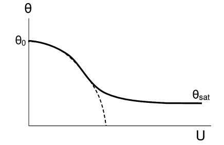
Figure 1: A schematic plot of electrowetting contact angle, $\theta(U)$. For zero voltage, the contact angle is the same as the Young angle, $\theta_{0}$. At low applied voltages $U$, the contact angle follows the Young-Lippmann formula, eq 6, (dashed line) $\cos\theta(U)-\cos\theta_{0}\simeq\cos\theta_{\rm YL}(U)-\cos\theta_{0}\sim U^{2}$, but for higher voltages the contact angle gradually deviates from the Young-Lippmann behavior and saturates towards some finite value, $\theta_{\rm sat}$.

When a small drop of liquid is placed on top of a solid surface it assumes the shape of a spherical cap Young_1805 . The contact angle $\theta_{0}$ between the drop and the surface, given by the Young formula DeGennesBook ; DeGennesReview ; Young_1805

$$\cos\theta_{0}=\frac{\gamma_{\rm sa}-\gamma_{\rm sl}}{\gamma_{\rm la}}$$ (1)

depends on the three interfacial tensions: solid/air $\gamma_{\rm sa}$, solid/liquid $\gamma_{\rm sl}$ and liquid/air $\gamma_{\rm la}$, where the air phase can be replaced by another immiscible fluid Ionization_1999 ; Microfluidics_Troian_2005 ; Berge_2000 .

The Young formula, eq 1, can be obtained by minimizing the capillary free energy with a fixed volume constraint DeGennesReview

$$F_{\rm cap}(\theta)=A_{\rm sa}\gamma_{\rm sa}+A_{\rm sl}\gamma_{\rm sl}+A_{\rm la}\gamma_{\rm la}-V\Delta P$$ (2)

where $A_{ij}$ are the interface areas between the $i$ and $j$ phases, $i,j=$ a (air), l (liquid), and s (solid); the drop volume is $V$ and the pressure difference across the liquid/air interface is $\Delta P$. For partial wetting, $\gamma_{\rm sa}<\gamma_{\rm sl}+\gamma_{\rm la}$, the capillary free energy $F_{\rm cap}$ has a minimum at the Young angle, $\theta_{0}$ [figure 2(a)].

Figure 2: Schematic plots of (a) the capillary free energy $F_{\rm cap}$ for a spherical drop of fixed volume and (b) a hypothetical (negative) total capacitance, $-C_{\rm tot}$, as function of contact angle $\theta$ in electrowetting setup. The minimum of the capillary term $F_{\rm cap}$ occurs at the Young angle $\theta_{0}$, while the electric term $F_{\rm el}=-\frac{1}{2}C_{\rm tot}U^{2}$ (or equivalently of $-C_{\rm tot}$) is assumed to have a minimum at a finite saturation angle, $\theta_{\rm sat}$.

The contact angle $\theta$ can be varied from its initial value $\theta_{0}$ by applying an external voltage of several volts to several hundreds of volts across the liquid drop. A commonly used electrowetting setup developed by Rinkel et al Mimmena_1980 and later perfected by Vallet et al Vallet_Berge_Vovelle_1996 is called electrowetting-on-dielectric (EWOD). The apparatus, roughly sketched in figure 3(a), includes a flat electrode as a substrate, which is coated with a thin dielectric layer (tens of nanometers to several micrometers thick), whose purpose is to prevent Faradic charge exchange (i.e., electrochemical reactions) at the electrode. It is common that this dielectric layer is then topped with an even thinner hydrophobic (i.e., Teflon) layer in order to control its surface tension. A drop of ionic solution is placed atop the coated electrode and a thin counter-electrode (usually a bare platinum fiber) is inserted into the drop from above. The drop is surrounded by air or by another immiscible dielectric liquid. Applying a voltage across the drop can cause a large change, of several tens of degrees, in the contact angle.

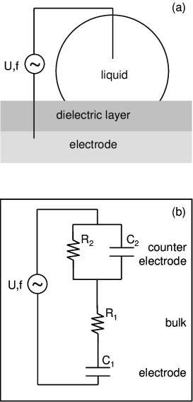
Figure 3: (a) A sketch of an EWOD setup with AC voltage $U$ of frequency $f$, and (b) its equivalent AC circuit. The two parallel-plate capacitors of capacitances $C_{1}$ and $C_{2}$ and areas $A_{1}$ and $A_{2}$ represent the substrate/liquid and the counter-electrode/liquid interfaces, respectively. The bulk liquid drop is represented by a resistor $R_{1}$ through which the two capacitors are charged and discharged. The charging time through the resistor is equal to the build-up time $\tau_{b}$ of the double-layers at the two interfaces. The discharge resistor $R_{2}$ represents the Faradic charge transfer processes that relax the electric double-layer near the counter-electrode with relaxation time $\tau_{r}$. Such mechanism is prevented at the substrate electrode because of its dielectric coating.

As reviewed in Ref 12, a simple relation between the contact angle and the applied voltage can be derived. When an external voltage $U$ is applied an electric double-layer is formed at the liquid/substrate interface. The total free energy $F_{\rm tot}$ has two contributions: a capillary term $F_{\rm cap}$, defined ft3 in eq 2, and an electric term, $F_{\rm el}$ that depends on $\theta$, $U$ and other system parameters.

$$F_{\rm tot}(\theta,U)=F_{\rm cap}(\theta)+F_{\rm el}(\theta,U)$$ (3)

Within the standard model of electrowetting (under external voltage control) the electric term is evaluated as

$$F_{\rm el}=-\frac{1}{2}C_{\rm ld}U^{2}$$ (4)

where $C_{\rm ld}$ is the capacitance of the liquid/substrate interface, which is modeled as a parallel-plate capacitor:

$$C_{\rm ld}\simeq\varepsilon_{0}A_{\rm ld}\left(\frac{d}{\varepsilon_{d}}+\frac{\lambda_{D}}{\varepsilon_{l}}\right)^{-1}\simeq\frac{\varepsilon_{0}\varepsilon_{d}}{d}A_{\rm ld}$$ (5)

where $A_{\rm ld}$ is the substrate area that is covered by the liquid drop, $d$ is the width of the dielectric layer and $\varepsilon_{d}$ and $\varepsilon_{l}$ are the dielectric constants of the dielectric coating and liquid drop, respectively. The Debye screening length, $\lambda_{D}$, is the width of the electric double-layer. In most cases, $d/\varepsilon_{d}\gg\lambda_{D}/\varepsilon_{l}$, and the second approximation in eq 5 can be justified. The parallel-plate capacitor model has been shown ITIES2_2006 to be valid as long as fringe fields are negligible ($d\ll A_{\rm ld}^{1/2}$) and the drop of volume $V$ is not too small for double-layers to be created ($\lambda_{D}\ll V^{1/3}$). An implicit assumption made in eq 4 is that the counter-electrode does not contribute to the total capacitance.

In an electrowetting setup, the contact angle $\theta(U)$ depends on the external voltage $U$. By substituting eq 5 into eq 4 and minimizing $F_{\rm tot}$ of eq 3 with a fixed volume constraint, the Young-Lippmann formula B2app_2005 for the contact angle $\theta_{\rm YL}(U)$ is obtained

$$\cos\theta_{\rm YL}(U)=\cos\theta_{0}+g^{-1}U^{2}$$ (6)

where $g^{-1}\equiv\varepsilon_{0}\varepsilon_{d}/(2\gamma_{\rm la}{d})$. It is a common practice to extend this DC voltage model to AC setups by using the rms voltage in eq 6, $U^{2}\to U^{2}_{\rm rms}$. Note that similar results can be obtained using force balance at the three-phase contact line Kang2002 .

Experiments ElectrostaticLimitations_Adamiak_2006 ; Jones_etal3_freq_2005 ; Jones_etal2_freq_2004 ; B2app_2005 ; papathanasiou_2007 ; ZeroCapillary_2005 ; Irreversibility_2009 ; finiteR_2003 ; Vallet_Berge_Vovelle_1996 ; Ionization_1999 ; Welters_Fokkink_1998 have shown that the $\sim U^{2}$ behavior predicted by the Young-Lippmann formula is indeed found for a range of low applied voltages, but the pre-factor of the $U^{2}$ term, eq 6, does not usually match the experimental data. For larger values of $U$, a deviation from the $U^{2}$ behavior is observed and a saturation in the contact angle, $\theta(U)\to\theta_{\rm sat}$, is reached gradually, as is schematically sketched in figure 1. In addition, it is convenient to define a characteristic value of the cross-over voltage $U^{*}$ by requiring that $\theta_{\rm YL}(U^{*})=\theta_{\rm sat}$ in eq 6:

$$\left(U^{*}\right)^{2}=g(\cos\theta_{\rm sat}-\cos\theta_{0})$$ (7)

Over the last decades, several models have been presented in an attempt to explain CAS B2app_2005 . Most of these models Ionization_1999 ; Fontelos_2009 ; papathanasiou_2005 ; papathanasiou_2007 ; finiteR_2003 ; ChargeTrapping_1999 are based on specific leakage mechanisms. Others, as in Ref 24, proposed heuristic arguments in order to predict CAS in electrowetting systems without relying on a specific mechanism.

Considering that the origin of CAS is not well understood from general principles, the objective of the present work is to offer a different approach to CAS, and to electrowetting in general. In the following section we consider the general circumstances in which CAS can occur intrinsically (without leakage). We present a low-voltage limit compatible with the Young-Lippmann quadratic voltage dependence and a high-voltage limit in which CAS is obtained. Furthermore, we identify a possibility for a novel electrowetting regime we call reversed electrowetting. In section III we present an application of this approach to EWOD experimental setups using a geometry-dependent model, and use AC circuit analysis to calculate the free energy. Section IV is dedicated to showing several numerical and analytical results and their compatibility with experiments. We conclude in section V with a summary along with some further discussion and an outlook on future research.

II A Generalized Model of Electrowetting

II.1 Generalized free energy and contact angle saturation

Our starting point is eq 3 above. Assuming that all the electric energy is stored via charge separation, it can be written in terms of the total capacitance, $F_{\rm el}=-\frac{1}{2}C_{\rm tot}U^{2}$. The total electrocapillary free energy $F_{\rm tot}$ is now written as

$$F_{\rm tot}(\theta,U)=F_{\rm cap}(\theta)-\frac{1}{2}C_{\rm tot}(\theta)U^{2}$$ (8)

where all capillary contributions are included in $F_{\rm cap}$. As $F_{\rm cap}$ is independent of $U$, the relative magnitude of the two terms in eq 8 is controlled by the negative $U^{2}$ dependence of the $F_{\rm el}$ term.

Physical insight can be gained from eq 8 by making different assumptions regarding the behavior of $C_{\rm tot}(\theta)$. Particularly, interesting results follow from the assumption that $C_{\rm tot}(\theta)$ has a maximum at some finite angle (see figure 2(b)), as will be shown below to be the case for EWOD setups. Our model therefore differs from previous models that took $C_{\rm tot}$ to be equal to $C_{\rm ld}$, (eq 4), which yields a monotonically decreasing $F_{\rm el}$. For reasons to be immediately apparent, we denote the angle where $C_{\rm tot}(\theta)$ has a maximum (or, equivalently, $F_{\rm el}$ has a minimum) as $\theta_{\rm sat}$. This angle, in general, is different from the Young angle, $\theta_{0}$, which minimizes the capillary term, $F_{\rm cap}$.

We now show how the existence of a global electric free-energy minimum at a finite contact angle yields CAS. With no applied voltage ($U=0$), $F_{\rm tot}=F_{\rm cap}$ and the system adheres to the Young angle, $\theta=\theta_{0}$, (figure 2(a)). Similarly, when the applied voltage $U$ is very large, the free energy is dominated by the electric term, $|F_{\rm el}|\propto U^{2}\gg F_{\rm cap}$, and the system tends towards $\theta_{\rm sat}$, which minimizes $F_{\rm el}$ (or, equivalently, maximizes $C_{\rm tot}$, figure 2(b)). Now, if the two contributions are concave for the accessible range of $\theta$, then the minimum of $F_{\rm tot}$ shifts smoothly from $\theta_{0}$ towards $\theta_{\rm sat}$ as $U$ is increased from zero to an arbitrary large value, as is schematically illustrated in figure 4. This description is consistent with CAS and implies that the saturation angle found in experiments can be identified with our definition of $\theta_{\rm sat}$.

Below we analyze more quantitatively the consequences of such a global electric minimum at the low- and high-voltage limits. In the former, we show a $\sim U^{2}$ variation of the contact angle with a pre-factor that can match the Young-Lippmann formula or be different from it. In the latter, an asymptotic $\sim U^{-2}$ approach to $\theta_{\rm sat}$ is found.

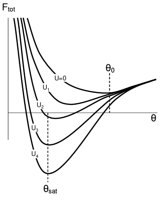
Figure 4: A schematic plot of the total free energy $F_{\rm tot}(\theta,U)=F_{\rm cap}(\theta)+F_{\rm el}(\theta,U)$, for a sequence of five applied voltages: $U_{4}>U_{3}>U_{2}>U_{1}>U=0$. Since the two energy terms are concave in the accessible range of $\theta$, their sum is also concave and has a minimum. Increasing $U$ from zero to a large $U_{4}$ causes a gradual shift of the minimum from $\theta_{0}$ towards $\theta_{\rm sat}$. Note that it cannot cross beyond $\theta_{\rm sat}$ regardless of how high the voltage $U$ is because $\theta_{\rm sat}$ is the minimum of the dominating $F_{\rm el}$ term.

II.2 The Low Voltage Limit

For $U\rightarrow 0$, the minimum of $F_{\rm tot}$ occurs close to $\theta_{0}$. Expanding this minimum condition $F^{\prime}_{\rm tot}(\theta)=0$ to first order in $\delta\theta=\theta(U)-\theta_{0}$, while recalling that $F^{\prime}_{\rm cap}(\theta_{0})=0$, we obtain

$$F^{\prime\prime}_{\rm cap}\left(\theta_{0}\right)\delta\theta-\frac{1}{2}U^{2}\left[C^{\prime}_{\rm tot}\left(\theta_{0}\right)+C^{\prime\prime}_{\rm tot}\left(\theta_{0}\right)\delta\theta\right]\simeq 0$$ (9)

yielding,

$$\delta\theta\simeq\frac{1}{2}\frac{C^{\prime}_{\rm tot}\left(\theta_{0}\right)}{F^{\prime\prime}_{\rm cap}\left(\theta_{0}\right)-\frac{1}{2}U^{2}C^{\prime\prime}_{\rm tot}\left(\theta_{0}\right)}U^{2}$$ (10)

and to leading order in $U^{2}$ one has

$$\theta(U)\simeq\theta_{0}+\frac{1}{2}\frac{C^{\prime}_{\rm tot}\left(\theta_{0}\right)}{F^{\prime\prime}_{\rm cap}\left(\theta_{0}\right)}U^{2}$$ (11)

and equivalently

$$\cos\theta(U)\simeq\cos\theta_{0}-\frac{1}{2}\frac{C^{\prime}_{\rm tot}\left(\theta_{0}\right)\sin\theta_{0}}{F^{\prime\prime}_{\rm cap}\left(\theta_{0}\right)}U^{2}$$ (12)

We see that at low voltages, the deviation from the Young angle is proportional to $U^{2}$, just as in the Young-Lippmann formula. However, the pre-factor is a function of $\theta_{0}$ and can take different values than in eq 6, and even change its sign (see section II.D). It is shown in section IV.D under which conditions the pre-factor converges to that of the Young-Lippmann formula for low voltages in typical EWOD experimental setups.

II.3 The High Voltage Limit

For $U\rightarrow\infty$, the electric energy becomes large relative to the capillary energy and so the minimum of $F_{\rm tot}$ occurs at $\theta(U)=\theta_{\rm sat}+\delta\theta$. Expanding the condition $F^{\prime}_{\rm tot}(\theta)=0$ around $\theta_{\rm sat}$, one has

$$F^{\prime}_{\rm cap}\left(\theta_{\rm sat}\right)+F^{\prime\prime}_{\rm cap}\left(\theta_{\rm sat}\right)\delta\theta-\frac{1}{2}C^{\prime\prime}_{\rm tot}\left(\theta_{\rm sat}\right)U^{2}\delta\theta\simeq 0$$ (13)

or

$$\theta(U) \simeq \theta_{\rm sat}+\frac{F^{\prime}_{\rm cap}(\theta_{\rm sat})}{\frac{1}{2}U^{2}C^{\prime\prime}_{\rm tot}(\theta_{\rm sat})-F^{\prime\prime}_{\rm cap}(\theta_{\rm sat})}$$ (14)

$$\simeq \theta_{\rm sat}+2\frac{F^{\prime}_{\rm cap}(\theta_{\rm sat})}{C^{\prime\prime}_{\rm tot}(\theta_{\rm sat})}U^{-2}$$

Hence, saturation in $\theta$ is approached asymptotically, as $U^{-2}$, in qualitative agreement with experiments B2app_2005 ; Romi_2008 .

II.4 Reversed Electrowetting

An interesting conclusion can be drawn from the discussion in section II.A. Recalling that in our model electrowetting results from an interplay between capillary and electric energies (each with its own minimum at $\theta_{0}$ and $\theta_{\mathrm{sat}}$, respectively), as voltage is increased the electric energy gradually becomes dominant and the contact angle is driven away from $\theta_{0}$ towards $\theta_{\mathrm{sat}}$ (figure 4). Since $\theta_{0}$ is determined only by the capillary parameters (as in the Young formula, eq 1) and $\theta_{\mathrm{sat}}$ is determined solely by the electric parameters, it is possible to envisage a system in which the saturation angle $\theta_{\rm sat}$ is actually larger than the Young angle, $\theta_{\mathrm{sat}}>\theta_{0}$ rather than $\theta_{\mathrm{sat}}<\theta_{0}$ as in the usual case. In such a setup, applying a voltage will cause an increase of the contact angle, in total contradiction with the Young-Lippmann formula, eq 6. Hence, the model proposed here allows for the possible existence of a new regime of electrowetting, which we refer to as reversed electrowetting.

By examining the slopes of each energy term near the minimum of the other (see figure 2), it is possible to show that in the low- and high-voltage limits, eqs 11 and 14, the pre-factors of both $U^{2}$ and $U^{-2}$ terms can take either positive or negative values depending on whether $\theta_{0}>\theta_{\mathrm{sat}}$ or $\theta_{0}<\theta_{\mathrm{sat}}$; for the low-voltage limit $F^{\prime\prime}_{\rm cap}\left(\theta_{0}\right)$ is positive by definition, but $C^{\prime}_{\rm tot}\left(\theta_{0}\right)$ is positive only if $\theta_{0}>\theta_{\mathrm{sat}}$ and negative for $\theta_{0}<\theta_{\mathrm{sat}}$. Likewise, for the high-voltage limit $C^{\prime\prime}_{\rm tot}\left(\theta_{\rm sat}\right)$ is negative by definition but $F^{\prime}_{\rm cap}\left(\theta_{\rm sat}\right)$ is negative only if $\theta_{0}>\theta_{\mathrm{sat}}$ and positive for $\theta_{0}<\theta_{\mathrm{sat}}$. Thus, we have shown how reversed electrowetting manifests itself in those limits.

III A Two Electrode Model of EWOD

Our goal in the remainder of this work is to elaborate on the physical conditions that are involved in determining a finite $\theta_{\rm sat}$ angle in specific EWOD experimental setups. However, we would like to stress that the proposed mechanism is general and may be applied to other realizations and experimental setups manifesting CAS.

III.1 System Setup & Geometry

A setup of an EWOD setup is presented in figure 5. The drop (dielectric constant $\varepsilon_{l}$) is assumed to retain its spherical-cap shape, with height $h$ from the surface, total volume $V$ and contact angle $\theta$. The metal electrode is coated with a dielectric layer of thickness $d$ and dielectric constant $\varepsilon_{d}$. The top counter-electrode is modeled as a thin cylinder of radius $b$ and the gap between the two electrodes is $h_{g}$. The two electrode areas covered by the liquid are $A_{1}$ and $A_{2}$, respectively. For spherical-cap shaped drops $A_{1}$ and $A_{2}$ are related to the contact angle $\theta$ through the fixed volume constraint:

$$A_{1} = \pi a^{2}$$

$$A_{2} = 2\pi b(h-h_{g})$$

$$\tan\frac{\theta}{2} = \frac{h}{a}$$

$$V = \frac{\pi h}{6}(3a^{2}+h^{2})$$ (15)

where $a$ is the radius of the covered portion of the substrate electrode.

It should be noted that $\theta$ can only take values in the range $\theta_{\rm min}<\theta<\pi$. The lower limit, $\theta_{\rm min}$, occurs when the drop height matches the gap between the lower tip of the counter-electrode and the substrate, $h=h_{g}$ (see figure 5), resulting in

$$\cot\frac{\theta_{\rm min}}{2}=\sqrt{\frac{2V}{\pi h_{g}^{3}}-\frac{1}{3}}$$ (16)

We will show that $\theta_{\rm sat}>\theta_{\rm min}$, hence $\theta_{\rm min}$ is an inaccessible lower bound of the contact angle. The upper limit $\theta=\pi$ is the de-wetting limit.

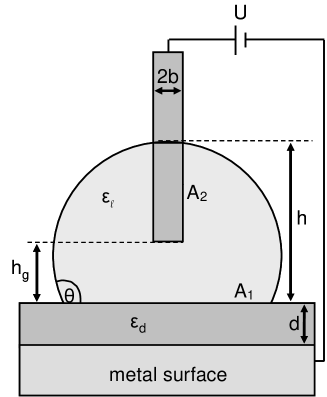
Figure 5: A schematic EWOD setup as used in our analysis. A liquid drop shaped as a spherical cap of volume $V$, height $h$ and dielectric constant $\varepsilon_{l}$ is placed atop a flat metal electrode. The metal electrode is covered with a dielectric coating of thickness $d$ and dielectric constant $\varepsilon_{d}$. A metal wire (used as a counter-electrode), modeled as a thin cylinder of radius $b$, is inserted into the drop from above. The gap between the two electrodes is $h_{g}$. The area of the substrate electrode covered by the drop is $A_{1}$ and that of the counter-electrode is $A_{2}$. The applied voltage is $U$ and the contact angle with the substrate is $\theta$.

III.2 The AC Free-Energy

The free energy, eq 8, depends on the total capacitance $C_{\rm tot}$, which includes all relevant contributions. Unlike the traditional Young-Lippmann treatment in which only the capacitance of the liquid/substrate interface is taken into account, we consider explicitly the existence of an additional double-layer, residing at the interface between the liquid drop and the counter-electrode.

Experimental setups and applications usually employ AC circuits to produce an electrowetting effect. Under those circumstances, double-layers are transient: with each AC half-cycle a double-layer of opposite polarity is formed at each electrode/liquid interface and subsequently dissolved away. In addition to relaxation by reversal of polarity, other mechanisms of relaxation can act at the counter-electrode/liquid interface such as electrochemical Faradic processes. The dynamical processes are, therefore, governed by two intrinsic time scales (beside the AC frequency):

1. The double-layer build-up time, $\tau_{b}$, which can be estimated to be

   $$\tau_{b}\simeq\frac{\lambda_{D}L}{D}$$ (17)

   where $\lambda_{D}=\sqrt{\varepsilon_{0}\varepsilon_{l}k_{B}T/2e^{2}c_{\rm salt}}$ is the Debye length, $k_{B}T$ the thermal energy, $c_{\rm salt}$ the salt concentration, $D$ is the diffusion constant and $L$ is a typical system size Bazant_2004 .

2. The double-layer relaxation time, $\tau_{r}$, which can similarly be expressed in terms of system parameters through the RC circuit relaxation formula

   $$\tau_{r}=R_{2}C_{2}=\rho\frac{C_{2}}{A_{2}}$$ (18)

   where $\rho=R_{2}A_{2}$ is defined as the zero-current (Faradic) resistivity to charge transfer by electrochemical processes and $A$ is the contact area.

In order to discuss the period-averaged properties of the system, we employ a standard AC circuit analysis. As shown in figure 3(b), we model the two liquid/electrode interfaces as two capacitors with capacitances ${C_{1},\,C_{2}}$, defined in a similar fashion as in eq 5:

$$C_{1} = C_{\rm ld}\simeq\frac{\varepsilon_{0}\varepsilon_{d}A_{1}}{d}$$

$$C_{2} \simeq \frac{\varepsilon_{0}\varepsilon_{l}A_{2}}{\lambda_{D}}$$ (19)

Note that the main contribution to $C_{1}$ comes from the coated dielectric layer of thickness $d$ ($d/\varepsilon_{l}\gg\lambda_{D}/\varepsilon_{l}$), while for $C_{2}$, the only contribution comes from the double layer of thickness $\lambda_{D}$ (because the counter-electrode is not coated). The cylindrical geometry of the counter-electrode is not considered because $b\gg\lambda_{D}$.

The two capacitors are charged and discharged through a resistor $R_{1}$ that represents the bulk of the liquid drop. The relaxation of the double-layer at the counter-electrode is modeled by an extra discharge circuit with a resistor $R_{2}$, while the capacitor $C_{1}$ does not have a discharge circuit since charge transfer at the substrate electrode is prevented by its dielectric coating. The appropriate resistance values can be inferred from the build-up ($\tau_{b}$) and relaxation ($\tau_{r}$) times, eqs 17 and 18, again through the RC circuit relaxation formula:

$$R_{1} = \tau_{b}(C_{1}^{-1}+C_{2}^{-1})$$

$$R_{2} = \frac{\tau_{r}}{C_{2}}$$ (20)

Drawing on the AC circuit analogy, the period-averaged free energy is:

$$F_{\rm tot}(\theta,U,\omega)=F_{\rm cap}+F_{\rm el}=F_{\rm cap}(\theta)-\frac{1}{2}\frac{1}{\omega\left|Z_{\rm tot}(\theta,\omega)\right|}U^{2}$$ (21)

where $U$ is understood to be the rms value and $Z_{\rm tot}$ is the total impedance of the circuit, [figure 3(b)], which can be represented schematically as

$$Z_{\rm tot}=Z_{C_{1}}\oplus Z_{R_{1}}\oplus(Z_{C_{2}}||Z_{R_{2}})$$ (22)

It is straight forward to show that the squared magnitude of the total impedance is

$$\left|Z_{\rm tot}\right|^{2} = \frac{1}{C_{1}^{2}}\left(\tau_{b}^{2}+\omega^{-2}\right)+\frac{2}{C_{1}C_{2}}\left(\tau_{b}^{2}+\frac{\tau_{r}(\tau_{r}+\tau_{b})}{1+\omega^{2}\tau_{r}^{2}}\right)$$ (23)

$$+ \frac{1}{C_{2}^{2}}\left(\tau_{b}^{2}+\frac{\tau_{r}(\tau_{r}+2\tau_{b})}{1+\omega^{2}\tau_{r}^{2}}\right)$$

Since $C_{1}$ is proportional to $A_{1}$, which vanishes at $\theta\rightarrow\pi$ and $C_{2}$ is proportional to $A_{2}$, which vanishes at $\theta\rightarrow\theta_{\mathrm{min}}$, $\left|Z_{\mathrm{tot}}\right|^{2}$ diverges both at $\theta\rightarrow\theta_{\mathrm{min}}$ and $\theta\rightarrow\pi$. Therefore, it must have a minimum at some intermediate value: $\theta_{\mathrm{min}}<\theta_{\mathrm{sat}}<\pi$. Hence, our model of electrowetting presented in section II.A is indeed applicable to typical EWOD setups.

Substituting eqs 15 and III.2 into eqs 21 and 23 yields an expression for $C_{1}(\theta)$ and $C_{2}(\theta)$ and, consequently, for $F_{\rm el}$ as a function of $\theta$. Its minimization can be done numerically (section IV.A) and yields the equilibrium contact angle (for given applied voltage and frequency). In some limits (sections IV.C and IV.E) analytical approximations can be derived as well.

IV Results and Discussion

IV.1 The Electrowetting Curve, $\theta(U)$

In order to demonstrate quantitatively the model validity, we performed numerical calculations for parameter values that are in accord with some typical experimental setups. In figure 6 we present the reactance $1/\omega Z$ (appearing in eq 21) computed for parameter values as in table 1 and with an AC frequency $f=\omega/2\pi=1$ kHz. The build-up time was calculated using eq 17 to be $\tau_{b}=1.34$ ms, while the relaxation time was calculated using eq 18 with ft7 $\rho=1\,\Omega\cdot m^{2}$, yielding ft6 $\tau_{r}=0.53$ s. For the chosen values of parameters, the ratio of capacitances for zero voltages ($\theta(U=0)=\theta_{0}$) is about, $C_{2}/C_{1}\simeq 25$. In the figure a maximum at a finite angle $\theta_{\rm sat}=53.3^{\circ}$ is clearly seen. Notably, this saturation angle is much larger than the minimal possible angle in this setup, $\theta_{\rm min}=37^{\circ}$ (see eq 16). As a consequence CAS is obtained for finite values of $A_{2}$, much before the limit $A_{2}\to 0$ characteristic to $\theta_{\rm min}$.

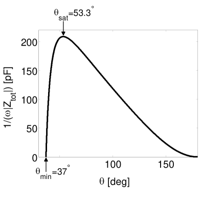
Figure 6: Total reactance $1/(\omega|Z_{\rm tot}|)$ (in nanoFarad) as a function of the contact angle. Parameters for the EWOD system are $\tau_{b}=1.34$ ms, $\tau_{r}=0.53$ s and $f=\omega/2\pi=1$ kHz, and all other parameters are chosen as in table 1. The reactance has a maximum for a finite value of $\theta_{\rm sat}=53.3^{\circ}$, at which the system exhibits CAS. The minimal contact angle is $\theta_{\rm min}=37^{\circ}$, eq 16.

Parameter	symbol	value
dielectric constant of liquid	$\varepsilon_{l}$	$80$
Debye length in liquid	$\lambda_{D}$	$1.34\textrm{nm}$
volume	$V$	$5\mu\textrm{L}$
width of dielectric layer	$d$	$0.1\mu\textrm{m}$
dielectric constant of dielectric layer	$\varepsilon_{d}$	$2.67$
liquid/air surface tension	$\gamma_{\rm la}$	$72.8\textrm{mN/m}$
dielectric/air surface tension	$\gamma_{\rm sa}$	$12.7\textrm{mN/m}$
liquid/dielectric interfacial tension	$\gamma_{\rm sl}$	$47\textrm{mN/m}$
gap between counter-electrode and substrate	$h_{g}$	$0.7\textrm{mm}$
radius of counter-electrode	$b$	$12.5\mu\textrm{m}$

Table 1: Parameter values of a typical electrowetting setup. The liquid drop contains an aqueous ionic solution and is placed on top of a Miyaline-C/Teflon substrate.

Figure 7 presents the calculated electrowetting curve $\theta(U)$ for the same system, where $\theta(U)$ is calculated by minimizing $F_{\rm tot}$ from eq 21, together with a plot of the Young-Lippmann formula (dashes), where an effective $g^{\rm eff}$ pre-factor is used to fit the full calculation. This is similar to what is done in many experimental works where the $g$ value is fitted from the low $U$ dependence, and not by using explicitly eq 6. We use a specific $g^{\rm eff}=(1+\omega^{2}\tau_{b}^{2})^{-1/2}$ as derived in section IV.D. The figure shows that several common experimental features are reproduced (as compared with the schematic figure 1); an initial compliance with the scaled Young-Lippmann formula at low voltages is followed by a cross-over at intermediate voltages to a different regime. Using eq 7 (with $g^{\rm eff}$), the cross-over voltage is evaluated to be $U^{*}\simeq 76.9$ V. At $U>U^{*}$ an asymptotic convergence of the contact angle towards a saturation value is seen, $\theta(U)\to\theta_{\rm sat}=53.3^{\circ}$. This is further demonstrated in figure 7, where the asymptotic $\theta(U)-\theta_{\rm sat}\sim U^{-2}$ is plotted (dotted line) following eq 14. The asymptotic behavior approximates rather well $\theta(U)$ for voltages larger than 120 V.

It is appropriate to define another voltage, $U_{\rm sat}$, characterizing the saturation range of the potential. An operational definition that we employ is that at $U_{\rm sat}$, the calculated $\theta(U_{\rm sat})$ deviates from $\theta_{\rm sat}$ by 2%. With this definition, we obtain $U_{{\rm sat}}\simeq 252.1$ V. The electrowetting curve presented in figure 7 agrees qualitatively with experimental observations FreqEW_2007 ; B2app_2005 ; Polarity_2006 , which show the effect of contact angle saturation. Unfortunately, because the parameter values needed for quantitatively comparison with experiments lack at present, we used instead reasonable estimations.

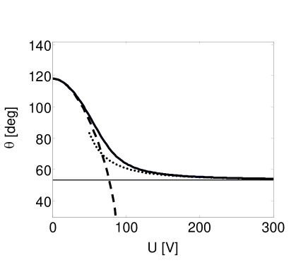
Figure 7: Calculated contact angle as a function of applied voltage, $U$ (full line), as well as a plot of the Young-Lippmann formula using $g^{\rm eff}$ (dashed line, see text). Parameter values of the EWOD system are taken from table 1 and $\tau_{b}=1.34$ ms, $\tau_{r}=0.53$ s and $f=\omega/2\pi=1$ kHz. Many of the features of CAS, shown schematically in figure 1, are reproduced. At $U=0$, the contact angle is $\theta_{0}=118^{\circ}$. For small $U$, there is an initial compliance with the rescaled Young-Lippmann formula, eq 6, $\theta(U)\approx\theta_{\rm YL}(U)$, followed by a cross-over occurring at $U^{*}=76.9$ V, calculated from eq 7. At larger $U$, the contact angle tends asymptotically to a saturation angle $\theta_{\rm sat}=53.3^{\circ}$. The asymptotic $\theta(U)-\theta_{\rm sat}\sim U^{-2}$ is plotted (dotted line) following eq 14 and approximates rather well $\theta(U)$ for voltages larger than 120 V. An operational definition of the saturation voltage $U_{\rm sat}$ (see text) yields $U_{\rm sat}\simeq 252.1$ V. Note that $\theta_{\rm sat}$ is conceivably larger than the minimal possible angle $\theta_{\rm min}=37^{\circ}$, eq 16.

IV.2 The Reversed Electrowetting Curve, $\theta(U)$

We now illustrate how reversed electrowetting $\theta_{\rm sat}<\theta_{0}$, which is a natural outcome of our model, can be seen in the laboratory. Let us consider a system similar to the one presented in the previous section with the two following changes (see table 2): the interfacial tensions are chosen such that $\theta_{0}=60^{\circ}$, and we now model a non-polar liquid with a dielectric constant $\epsilon_{l}=2$, which yields a build-up time of $\tau_{b}=1.34$ ms and a relaxation time of $\tau_{r}=13.2$ ms. The AC frequency is $f=\omega/2\pi=1$ kHz as before.

Figure 8 presents the calculated electrowetting curve $\theta(U)$. The plot features an initial compliance with the negatively rescaled Young-Lippmann formula (at low voltages such that the contact angle increases with the applied voltage. This is followed by a cross-over at intermediate voltages towards saturation. Using eq 7 (with $g^{\rm eff}$), the cross-over voltage is evaluated to be $U^{*}\simeq 65.5$ V. For $U>U^{*}$ an asymptotic convergence of the contact angle towards a saturation value is seen, $\theta(U)\to\theta_{\rm sat}=101.9^{\circ}$. Using the same definition as in section IV.A, the saturation voltage is found to be $U_{{\rm sat}}\simeq 208.5$ V.

Since our reversed electrowetting predictions (figure 7) are rather for specific parameter values, it will be of benefit to check their validity with experiments conducted on similar electrowetting setups.

Parameter	Value
$\varepsilon_{l}$	$2$
$\lambda_{D}$	$1.34\textrm{ nm}$
$V$	$5\textrm{ $\mu$L}$
$d$	$0.1\textrm{ $\mu$m}$
$\varepsilon_{d}$	$2.67$
$\gamma_{\rm la}$	$20\textrm{ mN/m}$
$\gamma_{\rm sa}$	$15\textrm{ mN/m}$
$\gamma_{\rm sl}$	$5\textrm{ mN/m}$
$h_{g}$	$0.7\textrm{ mm}$
$b$	$12.5\textrm{ $\mu$m}$

Table 2: Parameter values of a hypothetical system that exhibits reversed electrowetting.

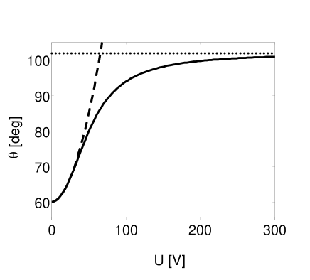
Figure 8: Calculated contact angle as a function of applied voltage, $U$, (solid line) for reversed electrowetting together with a manually scaled ($g^{\rm eff}<0$) Young-Lippmann formula (dashed line). Parameter values of a EWOD system are taken from table 2 and $\tau_{b}=1.34$ ms, $\tau_{r}=13.2$ ms and $f=\omega/2\pi=1$ kHz. At $U=0$, the contact angle is $\theta_{0}=60^{\circ}$. Even for small $U$, there is a deviation from the naive Young-Lippmann formula, eq 6, because $\theta(U)-\theta_{0}\sim U^{2}$, with a positive pre-factor. The $U^{2}$ rise is followed by a cross-over occurring at $U^{*}=65.5$ V. At larger $U$, the contact angle tends asymptotically to a saturation angle $\theta_{\rm sat}=101.9^{\circ}$. Using the same definition of the saturation voltage $U_{\rm sat}$ as in figure 7 yields $U_{\rm sat}\simeq 208.5$ V.

IV.3 The Frequency Dependence of Electrowetting

In order to explore the effect of the frequency of the AC voltage within our model, the dependence of the saturation angle $\theta_{\rm sat}$ on frequency was calculated numerically by minimizing eq 21 and plotted in figure 9 for several values of $\tau_{r}=0.53$ s, 0.053 s, and 5.3 ms. It can be seen that for this specific choice of parameters, the AC saturation angle reaches a constant value for the entire high frequency range down to $f\simeq 1$ kHz, even for the smallest of the chosen relaxation times ($\tau_{r}=5.3$ ms). Moreover, the larger $\tau_{r}$ is, the wider is the range for which the saturation angle is constant. This can be explained by taking into account that whenever $\tau_{r}\gg 1/f$, the counter-electrode double-layer can hardly relax.

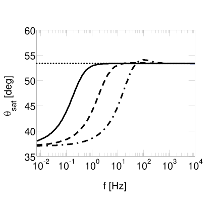
Figure 9: Saturation angle, $\theta_{\rm sat}$, as function of the AC frequency $f$, for the EWOD system with parameter values as in table 1, $\tau_{b}=1.34$ ms and for several $\tau_{r}$ values: $\tau_{r}=0.53$ s (solid line), 0.053 s (dashed line), 5.3 ms (dashed-dotted line). In the range $f\geq 1$ kHz, the AC saturation angle, which takes into account relaxation of the double-layer by electrochemical processes, matches the $\tau_{r}\to\infty$ (dotted line) of $\theta_{\rm sat}^{\infty}=53.3^{\circ}$ even for the smallest $\tau_{r}=5.3$ ms (fastest Faradic relaxation).

The frequency dependence of the contact angle has been experimentally studied in Ref 8 for several applied voltages. Figure 10 shows a comparison of a minimization of eq 23 for a range of frequencies, with experimental data. The calculations have been performed for system parameters as in table 3, which have been inferred ft1 from Ref 8, except for $\lambda_{D}=300$ nm, which was used as a fitting parameter to the experimental results. This value corresponds to ionic strength of less than $10^{-6}$ M and is compatible with de-ionized water used in Ref 8. The build-up time was deduced from the featured experimental results to be $\tau_{b}=0.1$ ms, and the relaxation time, $\tau_{r}=2.4$ ms, was calculated using eq 18 with $\rho=1\,\Omega\cdot m^{2}$.

Parameter	Value
$\varepsilon_{l}$	$80$
$\lambda_{D}$	$300\textrm{ nm}$ (fitted)
$V$	$5\textrm{ $\mu$L}$
$d$	$5\textrm{ $\mu$m}$
$\varepsilon_{d}$	$2.67$
$\gamma_{\rm la}$	$72.8\textrm{ mN/m}$
$\gamma_{\rm sa}$	$12.7\textrm{ mN/m}$
$\gamma_{\rm sl}$	$47\textrm{ mN/m}$
$h_{g}$	$0.7\textrm{ mm}$
$b$	$40\textrm{ $\mu$m}$

Table 3: Parameter values of an electrowetting system of de-ionized water solution on Miyaline-C/Teflon substrate. The parameter values are inferred from Ref 8, except for $\lambda_{D}$, which was fitted to obtain a quantitative agreement with experiments. The resulting value is indeed compatible with that of de-ionized water (ionic strength less than $10^{-6}$ M) ft1 .

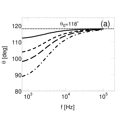
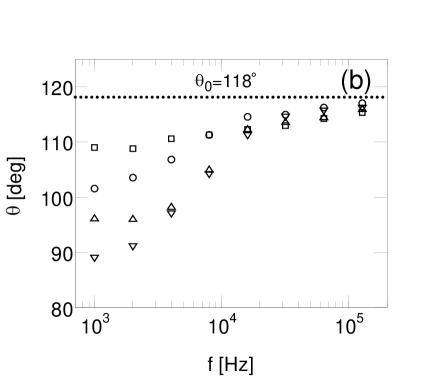
Figure 10: Contact angle as function of AC frequency $f$ for several applied voltages $U$. (a) Calculated values corresponding to 57 V (solid line), 93 V (short dashed line), 113 V (long dashed line) and 143 V (dashed-dotted line) with parameters as in table 3 and $\tau_{b}=0.1\textrm{ms},\,\tau_{r}=2.4\textrm{ ms}$. The value of $\theta_{0}=118^{\circ}$ is indicated by a dotted line. (b) Experimental results adapted from Ref 8 for the same voltages as in (a): squares (57 V), circles (93 V), triangles (113 V) and inverted triangles (143 V). A quantitative agreement between the calculation and experiment can be seen. Note also that the electrowetting effect diminishes at high frequencies as predicted analytically in eq 24.

Comparison of the two plots shows that our model reproduces rather well the frequency dependence found in experiments. It can be seen that the electrowetting effect diminishes with rising frequency, and seems to vanish at $f>100$ kHz where there is hardly any deviation from the Young angle. This can be easily understood taking into account that for $f>10$ kHz, $1/f$ becomes small as compared to the double-layer build-up time $\tau_{b}\simeq 0.1$ ms. Under those circumstances, ions move too slowly and cannot build considerable over-concentrations at the electrodes. Thus, at those high frequencies the period-averaged effect of the double-layers decreases considerably.

The above results imply that it is of value to further explore the limit of slow electrochemical processes, $\tau_{r}\gg\tau_{b}$, $\omega\tau_{r}\gg 1$, which leads to a simplified expression for the free energy. Substituting eq 23 into eq 21 we obtain in this limit

$$|Z_{\rm tot}| \approx \frac{\sqrt{\tau_{b}^{2}+\omega^{-2}}}{C_{\rm tot}(\theta)}$$

$$F_{\rm el}(\theta,U,\omega) = -\frac{1}{2\omega|Z_{\rm tot}|}U^{2}\approx-\frac{C_{\rm tot}(\theta)}{2\sqrt{1+\omega^{2}\tau_{b}^{2}}}U^{2}$$ (24)

where $C_{\rm tot}^{-1}=C_{1}^{-1}+C_{2}^{-1}$ is the total capacitance of an equivalent system without any electrochemical processes. The $(1+\omega^{2}\tau_{b}^{2})^{-1/2}$ pre-factor in eq 24 depends on the AC frequency and reflects a diminishing electrowetting effect for rising frequencies.

We note that the DC limit can be obtained by first assuming no electrochemical processes, $\tau_{r}\to\infty$ in eq 23 (leading to eq 24), and only then taking the DC limit of $\omega\to 0$ to get $F_{\rm el}=-\frac{1}{2}C_{\rm tot}U^{2}$ of eq 8. This limit can be useful in applications where both the substrate and counter-electrode are dielectrically coated.

If electrochemical processes are not totally excluded, but are just slow (order of seconds, in accordance with the value calculated in section IV.A), it is expected that the results obtained in this work will be applicable for that time scale, above which other mechanisms might take over. Such time-dependent behavior has been observed in Ref 24.

IV.4 Convergence to the Young-Lippmann Formula

In its DC limit ($\omega\rightarrow 0$), equation 24 provides a pathway to establish a relationship between our model and the Young-Lippmann formula and to show the conditions under which the two converge. Using eqs 15 and III.2 (see Appendix for more details), we have

$$C_{\mathrm{tot}}=C_{1}\left[1+\frac{C_{1}}{C_{2}}\right]^{-1}=C_{1}\left[1+\beta^{-1}\frac{2-\xi^{3}}{\xi^{2}-l^{-1}{h_{g}}\xi}\right]^{-1}$$ (25)

where $l\equiv({3V}/{\pi})^{1/3}$ is a typical drop length,

$$\beta\equiv\frac{6\epsilon_{l}db}{\epsilon_{d}\lambda_{D}l}$$ (26)

is a dimensionless parameter, and

$$\xi\equiv\left[\frac{1-\cos\theta}{2+\cos\theta}\right]^{1/3}$$ (27)

is a monotonically increasing function of $0\leq\theta\leq\pi$.

As long as the second term in the brackets of eq 25 is small, our model agrees with the standard model, $F_{\rm el}=-\frac{1}{2}C_{1}U^{2}$, eq 4, with $C_{1}=C_{\rm ld}$. For a typical system, as the one presented in table I, the value of the constant pre-factor is rather small $\beta^{-1}\simeq 0.01$. Since ${h_{g}}/{l}\leq\xi\leq 2^{\frac{1}{3}}$, it is clear that the quotient can only be large when $\xi\rightarrow h_{g}/l$ or, equivalently, when the contact angle becomes small enough. Otherwise, the second term is negligible and the two models converge.

Note that this view of the validity of the Young-Lippmann formula as being related to a certain range of the contact angles is a departure from the common approach which regards its validity being related to a certain range of applied voltages.

By creating this link between the Young-Lippmann formula and our model it can be deduced that the proper way of extending the Young-Lippmann formula (within its validity range) from DC to AC is to replace $U^{2}\to U^{2}_{\rm rms}/\sqrt{1+\omega^{2}\tau_{b}^{2}}$. This is exactly the how the Young-Lippmann formula was scaled (by $g^{\rm eff}$) in section IV.A.

IV.5 The Saturation Angle for Slow Relaxation ($\omega\tau_{r}\gg 1$, $\tau_{r}\gg\tau_{b}$)

Within the slow relaxation framework, eq 24, the minimization of $F_{\rm el}$ (yielding $\theta_{\rm sat}$) is equivalent to minimizing the total inverse capacitance $\alpha\equiv 1/C_{\mathrm{tot}}$. Using eqs 15 and III.2 we obtain

$$\alpha\left(\xi\right)=\frac{3d}{2\pi\varepsilon_{0}\varepsilon_{d}l^{2}}\left[\frac{1}{\xi^{-1}-\frac{1}{2}\xi^{2}}+\frac{2\beta^{-1}}{\xi-{l}^{-1}h_{g}}\right]$$ (28)

Minimizing $\alpha\left(\xi\right)$ yields a 6${}^{\text{th}}$ order polynomial in $\xi$:

$$\xi^{6}-2\beta\xi^{5}+4\beta l^{-1}h_{g}\xi^{4}$$ (29)

$$- 2\left(2+\beta l^{-2}h_{g}^{2}\right)\xi^{3}-2\beta\xi^{2}$$

$$+ 4\beta{l}^{-1}h_{g}\xi+2\left(2-\beta l^{-2}h_{g}^{2}\right)=0$$

It is possible to examine two separate limits for minimizing $\alpha\left(\xi\right)$, leading to two simple analytical expressions for $\theta_{\rm sat}$.

IV.5.1 Acute saturation angles (large $\beta$)

If $\xi^{3}\left(\theta_{\rm sat}\right)\ll 2$ then, near its minimum, eq 28 reduces to

$$\left.\alpha\right|_{\xi\simeq\xi_{\rm sat}}\simeq\frac{3d}{2\pi\varepsilon_{0}\varepsilon_{d}l^{2}}\left[\xi+\frac{2\beta^{-1}}{\xi-{l}^{-1}h_{g}}\right]$$ (30)

with a minimum at $\xi=\xi_{\rm sat}$ that satisfies

$$1-2\beta^{-1}\left(\xi_{\rm sat}-\frac{h_{g}}{l}\right)^{-2}=0$$ (31)

The solution yields

$$\xi_{\rm sat}=\sqrt{\frac{2}{\beta}}+\frac{h_{g}}{l}$$ (32)

and $\theta_{\rm sat}$ can now be obtained

$$\cos\theta_{\rm sat}=\frac{1-2\xi_{\rm sat}^{3}}{1+\xi_{\rm sat}^{3}}$$ (33)

Inserting typical values from table 1 to check for self-consistency, we get $\xi_{\rm sat}^{3}\approx 0.173\ll 2$ as required. Using eq 33 the saturation angle in this case is calculated to be $\theta_{\rm sat}\simeq 56.1^{\circ}$, which is not far from the value obtained by a full numerical calculation, $53.3^{\circ}$. As a rule of thumb we remark that the above condition, $\xi^{3}_{\rm sat}\ll 2$ holds for $\theta_{\rm sat}$ smaller than $\pi/2$, for which $\xi^{3}\left(\frac{\pi}{2}\right)=0.5\ll 2$.

IV.5.2 Large saturation angles (small $\beta$ and $h_{g}/l$)

For systems with small $\beta$ the above approximation should fail, as is apparent from eq 32. For such cases, we can use a different approximation assuming that the gap $h_{g}$ is small enough, such that

$$\xi_{\rm sat} \gg \frac{h_{g}}{l}$$ (34)

The saturation angle can then be found from a different approximated form of $\alpha(\xi)$ (eq 28), near its minimum:

$$\left.\alpha\right|_{\xi\simeq\xi_{\rm sat}} \simeq \frac{3d}{2\pi\varepsilon_{0}\varepsilon_{d}l^{2}}\left[\frac{1}{\xi^{-1}-\frac{1}{2}\xi^{2}}+\frac{2\beta^{-1}}{\xi}\right]$$ (35)

$$= \frac{3d}{\pi\varepsilon_{0}\varepsilon_{d}l^{2}}\left[\frac{1}{2-\xi^{3}}+\beta^{-1}\right]\xi^{-1}$$

Minimizing $\alpha(\xi)$, we get a quadratic equation in the variable $\xi^{3}$:

$$\xi^{6}-4\left(\beta+1\right)\xi^{3}+2\left(\beta+2\right)=0$$ (36)

whose solution is

$$\xi_{\rm sat}^{3}=2\left(\beta+1\right)\pm\sqrt{4\left(\beta+1\right)^{2}-2\left(\beta+2\right)}$$ (37)

For small $\beta$ it is possible to further simplify the expression for $\xi_{\rm sat}$ to obtain

$$\xi_{\rm sat}^{3}\simeq 2\left(1-\sqrt{\frac{3\beta}{2}}\right)$$ (38)

Checking for self-consistency, the condition holds for small enough gaps.

V Summary and Outlook

In this work we propose a novel approach towards electrowetting that, among other results, can account for contact angle saturation (CAS) applicable to some electrowetting setups. The model is based on a generalized version of the free energy accounting for various electric contributions. The interplay between the capillary ($F_{\rm cap}$) and electric ($F_{\rm el}$) terms depends on the applied voltage $U$, because $F_{\rm el}\sim-U^{2}$. Therefore, when an external voltage is applied it will drive the system away from its capillary free energy minimum and towards its electric free energy minimum.

Our approach is distinctly different from other views of electrowetting that make use of the Young-Lippmann formula. In our model the electric term can exhibit a variety of dependencies on the contact angle as determined by the exact system geometry. Particularly, if the electric term $F_{\rm el}$, has a global minimum at a certain contact angle $\theta_{\rm sat}$, then for high enough voltages this angle also minimizes (asymptotically) the total free energy, $F_{\rm tot}$. Additional increase of the applied voltage does not change the location of the global minimum and the contact angle saturates at $\theta_{\rm sat}$. We identify exactly this angle with the saturation angle found in experiments. This very general assumption ($F_{\rm el}$ with a minimum) is all that is needed to show that in the low-voltage limit a Young-Lippmann compatible $\sim U^{2}$ behavior is expected, while in the high-voltage limit a $\sim U^{-2}$ saturation should be present. Numerical calculations suggest that combination of these two limiting behaviors approximates rather well the full expression for $\theta(U)$ in the whole voltage range. in the whole voltage range.

When applying our approach to EWOD setups, we take two contributions to $F_{\rm el}$ into account: (i) the double-layer at the drop/substrate interface; and, (ii) another double-layer at the drop/counter-electrode interface. The latter was previously unaccounted for because it was considered to be negligible due to geometry, or that its relaxation time was considered to be very fast. However, we estimate the relaxation time to be long (on the order of seconds) and, therefore, the effect of the counter-electrode double-layer cannot be neglected for AC systems. Similarly, it cannot be neglected for low voltages (which will exclude electrochemical processes from taking place at all) lowV_2006 , or in DC applications that include a dielectrically coated counter-electrode. Using AC circuit analysis we show that $F_{\rm el}$ indeed has a global minimum that produces the CAS effect.

The value of the saturation angle as well as the entire electrowetting curve $\theta\left(U\right)$ can be found numerically for any choice of system parameters, and our specific choice is inspired by the experiments reviewed in Ref 12. There is a qualitative agreement with experimental results, which includes an initial compliance with the Young-Lippmann formula (scaled correctly), followed by a cross-over to CAS. The values obtained for the saturation angle, cross-over voltage and saturation voltage are also compatible with experimental values.

In addition, we investigated the frequency dependence of electrowetting. It is shown that the value of the saturation angle is independent of the AC frequency for a large range of frequencies (1 kHz to 100 kHz) for a specific choice of parameters. A numerical analysis of the frequency dependence of electrowetting was conducted for a set of system parameters inferred from Ref 8, and shows semi-quantitative agreement with the experiment. These results show that an approximation of the free energy can be justified, such that the entire frequency dependence is captured in a scaling factor of the applied voltage. It predicts that the electrowetting effect should diminish with rising frequency, as indeed found in experiments FreqEW_2007 .

In its DC limit our model can converge to the Young-Lippmann formula, depending on the values of the Young and saturation angles. We use this result to show a novel way to extend the Young-Lippmann formula from DC to AC systems. We conclude that the validity of the Young-Lippmann formula is related not to the range of applied voltages, as it is commonly viewed, but rather to the accessed range of contact angles. In commonly used EWOD setups, which are intentionally devised to have as high a Young angle and as low a saturation angle as possible (so the effect can be more easily measured), our model is compatible with a compliance to the Young-Lippmann formula at low voltages (and hence high contact angles). We note that the DC limit of our model can be most useful in DC applications that employ low voltages and/or include a dielectrically coated counter-electrode.

Our model does not rely on any leakage mechanisms to predict CAS. Nevertheless, we would like to stress that leakage mechanisms treated in previous works [7,22,26,31-33] can be added. Interestingly, it is conceivable that a cross-over between inherent CAS (as in the present model) and CAS originating from leakage mechanisms is responsible for the time-dependent saturation angle reported in Ref 24.

The fact that the saturation angle depends on electric parameters whereas the Young angle depends on the capillary parameters leads to the surprising possibility of reversed electrowetting. Therefore, it may be possible to construct a system in which the Young angle is lower than the saturation angle. In such a system the effect of applying an external voltage would be an increase in the contact angle — in total contradiction with the Young-Lippmann formula that allows only a decrease in the contact angle. We give an example of a choice of parameters that should yield reversed electrowetting.

Recently, the separate control of the Young and saturation angles was demonstrated in experiments Steckl_2010 . This ability was utilized to construct a set of dye cells dye_cell that are ‘complementary’ in their opposite response to applied voltage (black-to-white or vice-versa). We believe that further research in this direction will provide ample opportunity to test for the existence of reversed electrowetting. Finding such evidence would have a potential impact that can go much beyond our specific model.

We hope that some of the predictions presented in this paper will be tested in future experiments in a quantitative fashion, gaining more insight on electrowetting and the CAS phenomenon. For example, it will be interesting to study how retracting the counter-electrode and, hence, reducing its contact area $A_{2}$ affects the saturation angle, as well as coating it with a dielectric material. Our results suggest that more research into processes taking place at the counter-electrode is needed, especially with regards to CAS in DC EWOD setups.

Appendix A

It is convenient to express the geometrical parameters and the capacitances in terms of a monotonic function of the contact angle

$$\xi(\theta)=\left(\frac{1-\cos\theta}{2+\cos\theta}\right)^{1/3}$$ (39)

where $l=(3V/\pi)^{1/2}$, derived from the drop volume $V$, is a characteristic length.

The geometrical parameters defined in eq 15 can then be written as

$$h = l\xi(\theta)$$

$$a = \sqrt{\frac{1}{3}}l\left(2\xi^{-1}-\xi^{2}\right)^{1/2}$$

$$A_{1} = \frac{\pi l^{2}}{3}\left(2\xi^{-1}-\xi^{2}\right)$$

$$A_{2} = 2\pi bh_{g}\left(lh_{g}^{-1}\xi-1\right)$$ (40)

Combining the above expressions with the definitions of the two capacitances, we obtain

$$C_{1} = \frac{\pi}{3}\frac{\varepsilon_{0}\varepsilon_{d}l^{2}}{d}\left(2\xi^{-1}-\xi^{2}\right)$$

$$C_{2} = 2\pi bl\frac{\varepsilon_{0}\varepsilon_{l}}{\lambda_{D}}\left(\xi-l^{-1}h_{g}\right)$$ (41)

With the use of a dimensionless parameter

$$\beta=\frac{6\varepsilon_{l}}{\varepsilon_{d}}\frac{db}{\lambda_{D}l}$$ (42)

the ratio between the two capacitances can finally be expressed as:

$$\frac{C_{1}}{C_{2}}=\beta^{-1}\frac{2-\xi^{3}}{\xi^{2}-l^{-1}h_{g}\xi}$$ (43)

References

- (1) Rinkel, P. D.; Minnema, L.; Barneveld, H. A. IEEE Trans. Elec. Insu. 1980, 15, 461.
- (2) Jackle, J. A.; Hackwood, S.; Veselka, J. J; Beni, G. Applied Optics 1983, 22, 1765.
- (3) Gorman, C. B.; Biebuyck, H. A; Whitesides, G. M Langmuir 1995, 11, 2242.
- (4) Sondag-Huethorst, J. A. M.; Fokkink, L. G. J. Langmuir 1994, 10, 4830.
- (5) Vallet, M.; Berge, B.; Vovelle, L. Polymer 1996, 37, 2465.
- (6) Welters, W. J. J.; Fokkink, L. G. J. Langmuir 1998, 14, 1535.
- (7) Vallet, M.; Vallade, M.; Berge, B. Euro. Phys. J. B 1999, 11, 583.
- (8) Hong, J.S.; Ko, S. H.; Kang, K. H.; Kang, I. S. Microfluidics Nanofluidics 2007, 5, 263.
- (9) Monroe, C. W.; Urbakh, M.; Kornyshev, A. A. J. Phys. Cond. Mat. 2007, 19, 375113.
- (10) Monroe, C. W.; Daikhin, L. I.; Urbakh, M.; Kornyshev A. A. J. Phys.: Cond. Mat. 2006, 18, 2837; Monroe, C. W.; Daikhin, L. I.; Urbakh, M.; Kornyshev, A. A. Phys. Rev. Lett. 2006, 97, 136102.
- (11) Jones, T. B.; Fowler, J. D.; Chang, Y. S.; Kim C. J. Langmuir 2003, 19, 7646.
- (12) Mugele, F.; Baret, J. C. J. Phys.: Cond. Mat. 2005, 17, R705.
- (13) Herberth, U. Albert-Ludwigs University, Freiburg 2006, PhD thesis, (unpublished).
- (14) Shamai, R.; Andelman, D.; Berge, B.; Hayes, R. Soft Matter 2008, 4, 38.
- (15) Salata, O. V. Current Nanoscience 2005, 1, 25.
- (16) Pollack, M. G.; Fair, R. B.; Shenderov, A. D. Applied Phys. Lett. 2000, 77, 1725.
- (17) Darhuber, A. A.; Troian, S. M. Ann. Rev. Flu. Mech. 2005, 37, 425.
- (18) Feenstra, J.; Hayes, R. Liquivista Inc. internal communication 2006.
- (19) Berge, B.; Peseux, J. Eur. Phys. J. E 2000, 3, 159.
- (20) Esinenco, D.; Codreanu, I.; Rebigan, R. in Proceedings of International Semiconductor Conference 2006, 2, 443.
- (21) Adamiak, K. Microfluid Nanofluid 2006, 2, 471.
- (22) Shapiro, B.; Moon, H.; Garrell, R. L.; Kim, C. J.; J. App. Phys. 2003, 93, 5794.
- (23) Restolho, J.; Mata, J. L.; Saramago, B.; J. Phys. Chem. C 2009, 113, 9321.
- (24) Quinn, A. Sedev, R.; Ralston, J. J. Phys. Chem. B 2005, 109, 6268.
- (25) Quilliet, C.; Berge, B. Curr. Op. Coll. Int. Sci. 2001, 6, 34.
- (26) Verheijen, H. J. J.; Prins, M. W. J. Langmuir 1999, 19, 6616.
- (27) Berry, S.; Kedzierski, J.; Abedian, B. J. Coll. Interface Sci. 2006, 303, 517.
- (28) Millefiorini, S.; Tkaczyk, A. H.; Sedev, R.; Efthimiadis, J.; Ralston, J. J. Am. Chem. Soc. 2006, 128, 3098.
- (29) Jones, T. B.; Wang, K. L. Appl. Phys. Lett. 2005, 86, 054104.
- (30) Jones, T. B.; Wang, K. L.; Yao, D. J. Langmuir 2004, 20, 2813.
- (31) Papathanasiou, A. G.; Papaioannou, A. T.; Boudouvis, A. G. J. App. Phys. 2008, 103, 034901.
- (32) Fontelos, M. A.; Kindelan, U. Q. J. Mech. Appl. Math. 2009, 62, 465.
- (33) Papathanasiou, A. G.; Boudouvis, A. G. App. Phys. Lett. 2005, 86, 164102.
- (34) Young, T. Phil. Trans. R. Soc. Lond. 1805, 95, 65.
- (35) Quere, D.; de Gennes, P. G.; Brochard-Wyart, F.; Reisinger, A. Capillarity and Wetting Phenomena: Drops, Bubbles, Pearls, Waves, Springer, New-York, 2004.
- (36) de Gennes, P.G. Rev. Mod. Phys. 1985, 57, 827.
- (37) The contribution of the counter-electrode to the capillary energy can be neglected here based on its small dimensions.
- (38) K. H. Kang, K. H.; Langmuir 2002, 18, 10318-10322; Walker, S. W.; Shapiro, B. J. Microelectromech. Syst. 2006, 15, 986-1000; Schertzer, M. J.; Gubarenko, S. I.; Ben-Mrad, R.; Sullivan, P. E. Langmuir 2010, 26, 19230-19238; Cho, S. K.; Moon, H. J.; Kim, C. J. J. Microelectromech. Syst. 2003, 12, 70-79; Ren, H.; Fair, R.B.; Pollack, M. G.; Shaughnessy, E. J. Sens. Actuators B 2002, 87,201-206.
- (39) Bazant, M. Z. Thornton, K., Ajdari, A. Phys. Rev. E 2004, 70 021506.
- (40) According to Refs 41; 42 and 43, experiments on bio-sensors have shown that the zero-current Faradic resistivity of a number of metallic electrodes in standard saline ( mM/L) is of the order of . They further reported that these values stay in the same order of magnitude for current densities up to 0.1 . Since leakage currents in electrowetting experiments are much smaller, on the order of 0.1 (see Ref 31), the chosen values of can hence be justified.
- (41) Mayer, S.; Geddes, L. A.; Bourland, J. D.; Ogborn, L. Australas. Phys. Eng. Sci. Med. 1992, 15, 38.
- (42) Mayer, S.; Geddes, L. A.; Bourland, J. D.; Ogborn, L. Med. Biol. Eng. Comput. 1992, 30, 538.
- (43) Geddes, L. A.; Roeder, R. Annals Bio. Eng. 2001, 29, 181.
- (44) Note that this value means that the counter-electrode does not relax momentarily as is implied by the naive application of the Young-Lippmann formula to AC EWOD setups, which suggests .
- (45) , and are reported in Ref 8, while , , and are assigned reasonable values according to the materials used there, and and are estimated from photos it provides.
- (46) Kim, D. Y.; Steckl, A. J. Langmuir 2010, 26, 9474.
- (47) The dye cell of Ref 46 contains a drop of colored oil that is immersed in a transparent electrolyte. The two fluids compete to occupy the surface area of the substrate. Applied voltage changes the result of the competition. Such micron-scale dye cells can be embedded on a proper substrate to be used as electronic ink in e-paper applications.