Momentum Resolved Optical Lattice Modulation Spectroscopy for Bose Hubbard Model

Abstract

We propose a new method of optical lattice modulation spectroscopy for studying the spectral function of ultracold bosons in an optical lattice. We show that different features of the single particle spectral function in different quantum phases can be obtained by measuring the change in momentum distribution after the modulation. In the Mott phase, this gives information about the momentun dependent gap to particle-hole excitations as well as their spectral weight. In the superfluid phase, one can obtain the spectrum of the gapless Bogoliubov quasiparticles as well as the gapped amplitude fluctuations. The distinct evolution of the response with modulation frequency in the two phases can be used to identify these phases and the quantum phase transition separating them.

Ultracold atoms on optical lattices have opened up new possibilities of studying interacting quantum systems with tunable parameters in a controlled environment Bloch et al. (2008). A seminal achievement in this field has been the implementation of the Bose Hubbard model Jaksch et al. (1998), which is used as the paradigm for superfluid-insulator (SI) transitions, and has been studied extensively both analytically  Fisher et al. (1989); Sheshadri et al. (1993); Sengupta and Dupuis (2005); Freericks et al. (2009), and numerically Krauth and Trivedi (1991); Capogrosso-Sansone et al. (2007). The observation of the SI transition Greiner et al. (2002) in this system is a successful milestone in the study of ultracold atomic systems on optical lattices. More complex but related systems like Bose-Fermi mixtures Günter et al. (2006), spinor Bose condensates Sadler et al. (2006), and Bose Hubbard model with an artificial vector potential created by Raman beams Lin et al. (2009) have also been implemented leading to a host of novel phenomena  Jaksch (2008); Powell et al. (2010); Sinha and Sengupta (2010); Saha et al. (2010).

The SI transition in these systems is usually observed through time of flight images of boson density which yields information about the boson momentum distribution, $n_{\bf k}$, in the equilibrium state  Greiner et al. (2002). The superfluid phase is then identified by sharp peaks of $n_{\bf k}$ at zero momentum (and at corresponding Bragg vectors), while the Mott phase shows a diffuse density pattern. The contrast of the peaks (or visibility) has traditionally been used to track such SI transitions. This is, however, unsatisfactory for a clean distinction between the two quantum phases. The main problem with this method, as pointed out in earlier works Diener et al. (2007), is that $n_{\bf k}$ has a precursor peak at ${\bf k}=0$ near the SI transition  Sengupta and Dupuis (2005). Thus looking for a signature of superfluidity involves looking for an extra peaky feature on top of the generalized cluster around ${\bf k}=0$ which is experimentally challenging. The other approach that has been suggested is to measure the local density in situ with a very fine resolution and look for a plateau of constant density corresponding to the Mott phase  Ho and Zhou (2009); Gemelke et al. (2009). An alternate direct way of distinguishing between the superfluid and Mott phases is to measure the excitation spectra in these two phases. The superfluid phase has gapless spectrum with a linear low energy dispersion, while the spectrum in the Mott phase is gapped. Indeed the energy transfer due to optical lattice modulation Jördens et al. (2008); Huber and Rüegg (2009); Sensarma et al. (2009) has been previously studied as a possible probe for the Bose Hubbard model Kollath et al. (2006); Huber et al. (2007). However, such a method does not yield momentum-resolved information about the spectral function of the bosons.

In this letter, we propose a novel method based on optical lattice modulation Jördens et al. (2008); Huber and Rüegg (2009); Sensarma et al. (2009) to obtain the single particle spectral properties of the Bose-Hubbard model in both the Mott and the superfluid phases. (In a broad qualitative sense, our proposed technique, as we establish in this work, is somewhat akin to being the bosonic counterpart of the ARPES technique used extensively in solid state electronic materials in the sense that our method gives direct momentum- and frequency-resolved spectral information about the low-lying quantum excitations of the interacting system.) Our proposed experiment is the following: we turn on an additional weak modulating optical lattice at frequency $\omega$ for some time before turning off all lattice and trap potentials simultaneously and measuring the density of the particles after a time of flight. For a sufficiently long time of flight, the density in real space can be mapped back to the momentum distribution of the system after the lattice modulation. We propose to compare this momentum distribution to that in the unperturbed case (without the modulation). We note at the outset that such a comparison of momentum distributions involves looking at the excitations created by the optical lattice modulation and not measuring equilibrium $n_{\bf k}$ of the bosons. Hence the proposed experiment does not suffer from the problem of measuring the equilibrium $n_{\bf k}$ mentioned earlier. We show that the change in the momentum distribution as a function of modulating frequency $\omega$, $\delta n_{\bf k}(\omega)$, carries information about the interacting spectral function both in the Mott and the superfluid side of the phase diagram. Using a non-perturbative strong coupling expansionSengupta and Dupuis (2005), we compute $\delta n_{\bf k}(\omega)$ and provide a precise algorithm to extract spectral information from the measurement. We demonstrate that in the Mott phase, the variation of $\delta n_{\bf k}(\omega)$ in the Brillouin zone with $\omega$ tracks the dispersion of the gapped particle-hole excitations while in the superfluid phase, $\delta n_{\bf k}$ shows a gapless linear dispersion at low $\omega$ and a gapped amplitude mode at high $\omega$. This leads to a qualitative distinction between the two phases. The height of the peaks of $\delta n_{\bf k}$ in the Brillouin zone also contain important information about the spectral weights of the different modes. Note that our proposed method contains detailed momentum resolved information which is not accessible by looking at the total energy transferred by lattice modulation suggested earlier Kollath et al. (2006); Huber et al. (2007). Recently the study of these spectral features through Bragg spectroscopy (which measures the structure factor) has been suggested and the corresponding response functions have been calculated Huber et al. (2007). However, compared to Bragg spectroscopy, our method is simpler to implement as it does not require additional lasers and the data can be collected in a single shot. Additionally, our method can yield momentum resolved spectral information, while Bragg spectroscopy integrates over the single particle momenta. Thus our proposal constitutes a significant improvement over the existing experimental proposals for both accurate detection of the SI transition and for obtaining the momentum-resolved spectral information for bosonic excitations in ultracold atom systems.

We consider an ultracold atomic implementation of a repulsive Bose Hubbard model on a d-dimensional hypercubic optical lattice described by the Hamiltonian

$$H=-J\sum_{\langle ij\rangle}b^{\dagger}_{i}b_{j}+U\sum_{i}n_{i}(n_{i}-1)-\mu\sum_{i}n_{i},$$ (1)

where $b^{\dagger}_{i}$ creates a boson on the site $i$ and $n_{i}=b^{\dagger}_{i}b_{i}$ is the number operator on site $i$, and we shall focus on $d=2,3$ in the present work. Here $J$, $U$ and $\mu$ are respecively the tunneling parameter, the onsite repulsion and the chemical potential of the system. At $T=0$ this system undergoes a SI transition as a function of $J/U$ (or density or equivalently $\mu/U$) with the Mott insulating phase occuring at small $J/U$ and at a commensurate integer density on each site. On top of this system, we consider a small perturbation to the optical lattice potential modulated at a frequency $\omega$. Since the tunneling is exponentially dependent on the height of the optical lattice while other parameters have much weaker dependence, the primary effect of this perturbation is to modulate the tunneling parameter. The perturbing Hamiltonian can then be written as

$$H_{1}=-\lambda J\cos(\omega t)\sum_{\langle ij\rangle}b^{\dagger}_{i}b_{j},$$ (2)

where $t$ denotes time and $\lambda$ is a small perturbation parameter. For a deep lattice, $J\sim E_{R}exp(-\sqrt{V_{0}/E_{R}})$ where $V_{0}$ is the lattice height and $E_{R}$ is the recoil energy. Hence $\lambda\sim\sqrt{V_{0}/E_{R}}\delta V_{0}/V_{0}$, where $\delta V_{0}$ is the amplitude of modulation of the optical lattice height. This gives an order of magnitude for $\lambda$. More quantitatively accurate estimates can be easily obtained by solving the band structure problem.

Figure 1: The out of phase response of the momentum distribution in the $n=1$ Mott phase of 2D Bose Hubbard model ($U=30J$ and $\mu=20J$) for (a)$\omega=20J$ and (b) $\omega=35J$. (c) and (d): Integrated response from 3D Bose Hubbard model ($U=40J$ and $\mu=10.5J$) for (c) $\omega=20J$ and (b) $\omega=45J$. The perturbation parameter $\lambda=0.1$ for all the plots. (Color online)

We begin with the Mott phase of the model. Within linear response (linear in $\lambda$), the change in $n_{\bf k}$ is

$$\delta n_{\bf k}(t)=n_{1}({\bf k},\omega)\cos\omega t+n_{2}({\bf k},\omega)\sin\omega t,$$ (3)

where the in phase and out of phase response of the system, $n_{1}$ and $n_{2}$, are given by the real and imaginary part of the response function $\Pi({\bf k},\omega+i0^{+})$ with

$$\Pi({\bf k},i\omega)=-\frac{1}{\beta}\epsilon_{\bf k}\sum_{i\omega_{n}}G({\bf k},i\omega_{n})G({\bf k},i\omega+i\omega_{n}).$$ (4)

Here $\beta=1/T$, $T$ being the temperature of the system, $\epsilon_{\bf k}=-2J\sum_{i=1,d}\cos k_{i}$ is the bare band dispersion of the system and $G({\bf k},\omega)$ is the single-particle Green function of the system. The response function in eq. 4 neglects vertex corrections although self-energy corrections can be included in the Green functions used to evaluate it. Note that for a non-interacting system $n_{2}$ is identically zero as the perturbation commutes with the non-interacting Hamiltonian.

The single particle Green function in the Mott phase within the random phase approximation (RPA) Sengupta and Dupuis (2005) is given by

$$G({\bf k},i\omega)=z_{\bf k}(i\omega-E^{+}_{\bf k})^{-1}+(1-z_{\bf k})(i\omega-E^{-}_{\bf k})^{-1},$$ (5)

where the particle (hole) dispersions are given by $E^{+(-)}_{\bf k}=-\delta\mu+\frac{1}{2}\left(\epsilon_{\bf k}\pm\sqrt{\epsilon_{\bf k}^{2}+4\epsilon_{\bf k}Ux+U^{2}}\right)$ and the spectral residue is given by $z_{\bf k}=(E^{+}_{\bf k}+\delta\mu+Ux)/(E^{+}_{\bf k}-E^{-}_{\bf k})$. Here $x=n+1/2$ and $\delta\mu=\mu-U(n-1/2)$ where $n$ is the integer number of bosons on each site. Using the above form of the boson Green function, we then obtain

$$n_{1}({\bf k},\omega) = 2\lambda\epsilon_{\bf k}\frac{\Delta_{\bf k}z_{\bf k}(1-z_{\bf k})[n_{B}(E^{-}_{\bf k})-n_{B}(E^{+}_{\bf k})]}{\omega^{2}-\Delta_{\bf k}^{2}},$$

$$n_{2}({\bf k},\omega) = \pi\lambda\epsilon_{\bf k}z_{\bf k}(1-z_{\bf k})[n_{B}(E^{-}_{\bf k})-n_{B}(E^{+}_{\bf k})]$$ (6)

$$\times[\delta(\omega+\Delta_{\bf k})-\delta(\omega-\Delta_{\bf k})],$$

where $\Delta_{\bf k}=E^{+}_{\bf k}-E^{-}_{\bf k}$ is the momentum dependent gap to creating particle-hole excitations in the system with zero center of mass momentum and $n_{B}$ is the Bose distribution function. It is clear from the form of $\Delta_{\bf k}$ that it has the lowest (but finite) value $\Delta_{M}$ at the zone center (${\bf k}=[0,0]$) and increases as we go out towards the edge of the Brillouin zone. The SI transition is then marked by the vanishing of $\Delta_{M}$

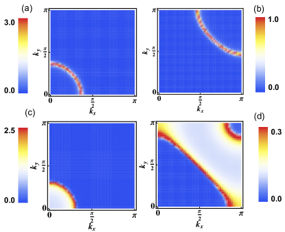
We focus here on $n_{2}({\bf k},\omega)$, which shows sharp features in the response. For modulation frequencies below the Mott gap, $n_{2}({\bf k},\omega)$ is zero everywhere in the Brillouin zone. For frequencies above the Mott gap $n_{2}$ will have response at the contours corresponding to $\Delta_{\bf k}=\omega$ with a weight proportional to $z_{\bf k}(1-z_{\bf k})$. Looking at $n_{1}({\bf k},\omega)$, we see that for frequencies less than the Mott gap, the response is broad with a broad peak at the zone center. For frequencies above the Mott gap, the response is sharply peaked around the contours of $\Delta_{\bf k}=\omega$ and changes sign as this contour is crossed. This qualitative reasoning is verified in Fig. 1(a) and (b), where $n_{2}({\bf k},\omega)$ is plotted as a function of $k_{x}$ and $k_{y}$ for $d=2$ and two different frequencies corresponding to (a) $\Delta_{M}<\omega<U$ and (b) $\omega>U$. For frequencies above the Mott gap, we see a contour of excitations which moves from the zone center to the edge of the Brillouin zone as the frequency is increased. Thus, one can determine the momentum dependent gap by doing a frequency sweep and looking at the peaks in the response. We note that for the 3D Bose-Hubbard model, the measured momentum distribution is integrated along one axis and hence an analogous plot will reflect $\int_{-\pi}^{\pi}dk_{z}n_{2}({\bf k},\omega)/2\pi$. The column integration leads to a region of excitations with the perimeter defined by the contour of excitations in the $k_{x}-k_{y}$ plane. This is plotted in Fig. 1 (c) and (d), for two different values of $\omega$.

Figure 2: (a) and (b) : The out of phase response of the momentum distribution in the superfluid phase for a 2D Bose Hubbard model ($U=5J$ and $\mu=2.3J$) for (a) $\omega=4J$ (b) $\omega=7J$. In (a) the response is due to creation of two phase modes. In (b) the low ${\bf k}$ response is from simultaneous excitation of a phase and an amplitude mode. There is also a small response from excitation of two phase modes at large ${\bf k}$. (c) and (d): Column integrated out of phase response for 3D Bose Hubbard model ($U=8J$ and $\mu=2.2J$) for (c) $\omega=4.2J$ (b) $\omega=11.2J$. The rings seen in the 2D response are now filled up due to column integration. The perturbation parameter $\lambda=0.1$ for all plots.(Color online)

We now turn our attention to the superfluid phase, which is characterized by the presence of a macroscopic condensate and finite expectation values of the anomalous propagators $F({\bf k},i\omega_{n})=\langle b^{\dagger}_{\bf k}b^{\dagger}_{-{\bf k}}\rangle$. In this case, the response function $\Pi({\bf k},i\omega)$ in Eq. 4 has an extra term coming from the anomalous propagators and is given by

$$\Pi({\bf k},i\omega_{n}) = -\frac{1}{\beta}\epsilon_{\bf k}\sum_{i\omega_{n}}\big{[}G({\bf k},i\omega_{n})G({\bf k},i\omega+i\omega_{n})$$ (7)

$$+ F({\bf k},i\omega_{n})F({\bf k},i\omega-i\omega_{n})\big{]}.$$

In the superfluid phase, the normal and the anomalous Green functions are given by Sengupta and Dupuis (2005)

$$G({\bf k},i\omega_{n}) = \frac{g_{1{\bf k}}}{i\omega_{n}-E_{1{\bf k}}}+\frac{g_{2{\bf k}}}{i\omega_{n}+E_{1{\bf k}}}$$

$$+\frac{g_{3{\bf k}}}{i\omega_{n}-E_{2{\bf k}}}+\frac{g_{4{\bf k}}}{i\omega_{n}+E_{2{\bf k}}},$$

$$F({\bf k},i\omega_{n}) = \Phi\left[\frac{f_{{\bf k}}}{i\omega_{n}^{2}-E_{1{\bf k}}^{2}}+\frac{1-f_{{\bf k}}}{i\omega_{n}^{2}-E_{2{\bf k}}^{2}}\right],$$ (8)

where $E^{2}_{1(2){\bf k}}=-B_{\bf k}\pm\sqrt{B_{\bf k}^{2}-C_{\bf k}}$ with $B_{\bf k}=b_{\bf k}-a_{\bf k}^{2}/2+\Phi^{2}/2$ and $C_{\bf k}=b_{\bf k}^{2}-\Phi^{2}(\mu+U)^{2}$. Here $a_{\bf k}=2\delta\mu-\epsilon_{\bf k}-2\Phi$, $\Phi=\frac{\delta\mu^{2}-U^{2}/4}{\mu+U}+zJ$, and $b_{\bf k}=\delta\mu^{2}-U^{2}/4-(\epsilon_{\bf k}+2\Phi)(\mu+U)$, with $z=2d$ for a hypercubic lattice in d dimensions. The quasiparticle weights are given by $g_{1(2){\bf k}}=[E_{1{\bf k}}\pm(\mu+U)][E_{1{\bf k}}^{2}\mp a_{\bf k}E_{1{\bf k}}+b_{\bf k}]/(2E_{1{\bf k}}[E_{1{\bf k}^{2}}^{2}-E_{2{\bf k}}^{2}])$, $g_{3(4){\bf k}}$ is obtained from $g_{1(2){\bf k}}$ by taking $E_{1{\bf k}}\leftrightarrow E_{2{\bf k}}$, and $f_{{\bf k}}=(E_{1{\bf k}}^{2}-(\mu+U)^{2})/(E_{1{\bf k}}^{2}-E_{2{\bf k}}^{2})$. The pole $E_{2{\bf k}}$ is the gapless phase fluctuation mode at small ${\bf k}$ (near the zone center). The pole $E_{1{\bf k}}$ represents the amplitude mode at low ${\bf k}$ and is gapped. At large ${\bf k}$ the amplitude and phase modes are mixed; however, we still refer to these modes as amplitude and phase mode for easy identification. The phase mode carries almost all the spectral weight at low ${\bf k}$, while the spectral weight resides mainly in the gapped mode at larger ${\bf k}$ values.

Using these forms for the propagators we can now evaluate the momentum distribution response function. For simplicity, we restrict ourselves to $T=0$ and $\omega>0$ (note that the in-phase and out of phase responses are respectively symmetric and antisymmetric in $\omega$). Then, the change in momentum distribution is given by

$$n_{1}({\bf k},\omega) = 2\pi\lambda\epsilon_{\bf k}\left[\nu_{\bf k}\frac{E_{1{\bf k}}+E_{2{\bf k}}}{\omega^{2}-(E_{1{\bf k}}+E_{2{\bf k}})^{2}}\right.$$

$$\left.+\alpha_{\bf k}\frac{2E_{1{\bf k}}}{\omega^{2}-4E_{1{\bf k}}^{2}}+\beta_{\bf k}\frac{2E_{2{\bf k}}}{\omega^{2}-4E_{2{\bf k}}^{2}}\right],$$

$$n_{2}({\bf k},\omega) = \pi\lambda\epsilon_{\bf k}\left[\nu_{\bf k}\delta(\omega-E_{1{\bf k}}-E_{2{\bf k}})\right.$$

$$\left.+\alpha_{\bf k}\delta(\omega-2E_{1{\bf k}})+\beta_{\bf k}\delta(\omega-2E_{2{\bf k}})\right],$$

where $\nu_{\bf k}=-g_{1{\bf k}}g_{4{\bf k}}-g_{2{\bf k}}g_{3{\bf k}}+\Phi^{2}f_{\bf k}(1-f_{\bf k})/(2E_{1{\bf k}}E_{2{\bf k}})$, $\alpha_{\bf k}=-g_{1{\bf k}}g_{2{\bf k}}+\Phi^{2}f_{\bf k}^{2}/(4E_{1{\bf k}}^{2})$, and $\beta_{\bf k}=-g_{3{\bf k}}g_{4{\bf k}}+\Phi^{2}(1-f_{\bf k})^{2}/(4E_{2{\bf k}}^{2})$.

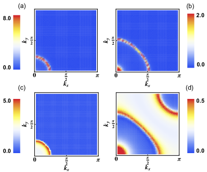
Eq. Momentum Resolved Optical Lattice Modulation Spectroscopy for Bose Hubbard Model shows that the out of phase response in the SF phase is peaked at energies corresponding to the creation of (a) two phase modes (b) an amplitude and a phase mode and (c) two amplitude modes. The in-phase response also shows broader peaks at these contours. At low frequencies (less than the gap in $E_{1{\bf k}}$), the experiments should see a single contour of excitations corresponding to two phase mode excitations, as shown in Fig 2(a) for $d=2$. As the frequency crosses the gap of the amplitude mode, two contours should be visible, a large contour corresponding to two phase modes and a small ${\bf k}$ contour corresponding to an amplitude and a phase mode, as in Fig 2(b). As the frequency crosses twice the gap, the two phase modes disappear as the frequency is above their bandwidth. The large ${\bf k}$ response is due to one amplitude and one phase mode. There is a low ${\bf k}$ response from two amplitude modes, but it is heavily suppressed due to spectral weights. For $d=3$, a similar pattern is observed. However, the contours are replaced by regions with boundaries given by the location of the corresponding excitations in the $k_{x}-k_{y}$ plane, as shown in Fig. 2(c) and (d).

Thus we see that the change in momentum distribution due to optical lattice modulation can be used to obtain the excitation spectrum in both the Mott and the superfluid phase. In the Mott phase, the particle-hole spectrum is gapped and there is no low frequency response. For both $d=2$ and $3$ and for modulation frequencies above the Mott gap, the response is peaked at the contour in the Brillouin zone whose dispersion matches the modulation frequency. Thus the peak response occurs on contours of increasing size as the frequency is increased. On the other hand, in the superfluid phase, the existence of gapless phase modes leads to low frequency response on contours whose size increase with frequency. However, on crossing the gap for the amplitude mode, there is a large response near the zone center and two distinct contours can be seen in this regime. At higher frequencies, there is a third contour of excitations corresponding to two amplitude modes, where the response is suppressed due to low spectral weight.

In conclusion, we have derived the response of the momentum distribution of a Bose Hubbard model to optical lattice modulation within a strong coupling expansion, both in the Mott insulator and the superfluid phase. In real experiments, the sharp poles in the single particle Green functions will be smeared due to several factors leading to a broadening of the response shown. The harmonic trap will smear the distribution on a momentum scale of the order of the inverse oscillator length scale. For a wide trap, this is usually negligible compared to other sources of smearing. Finite temperature will lead to a smearing on energy scales $\sim T$. For the Mott insulating phase, this smearing would be negligible as long as the temperature is much smaller than the Mott gap ($T\ll U$) Gerbier (2007); Weld et al. (2009), which is easily achievable experimentally. For the superfluid phase, the low energy excitations would be smeared and it would be impossible to follow the very long wavelength low energy response (below energy $\sim T$). However, the strong momentum dependence of the spectral weight of the phase modes would still lead to relatively well defined peaks in the Brillouin zone. On the other hand, deep in the superfluid phase, the amplitude modes are gapped and the emergence of the small contour around the gap frequency should be easy to observe. Finally, including vertex corrections on top of the random phase approximation would broaden the poles, especially for the amplitude modes. The broadening represents processes where the amplitude mode can decay into two or more phase modes. However, for lattice systems, the phase modes have a finite bandwidth and a large gap for the amplitude mode restricts the phase space for such processes. Further, the two phonon decay involves phonon modes at relatively large energies which carry very little spectral weight. Thus the amplitude modes would be sharply defined near the zone center and hence the emergence of the small response contour around the gap should be easily observable.

R.S. and S.D.S. acknowledges support from ARO-DARPA-OLE, ARO-MURI and JQI-NSF-PFC. K.S. thanks DST, India for support through project no. SR/S2/CMP-001/2009.

References

- Bloch et al. (2008) I. Bloch, J. Dalibard, and W. Zwerger, Rev. Mod. Phys. 80, 885 (2008).
- Jaksch et al. (1998) D. Jaksch, C. Bruder, J. I. Cirac, C. W. Gardiner, and P. Zoller, Phys. Rev. Lett. 81, 3108 (1998).
- Fisher et al. (1989) M. P. A. Fisher, P. B. Weichman, G. Grinstein, and D. S. Fisher, Phys. Rev. B 40, 546 (1989).
- Sheshadri et al. (1993) K. Sheshadri, H. Krishnamurthy, R. Pandit, and T. Ramakrishnan, Euro. Phys. Lett. 22, 257 (1993).
- Sengupta and Dupuis (2005) K. Sengupta and N. Dupuis, Phys. Rev. A 71, 033629 (2005).
- Freericks et al. (2009) J. K. Freericks, H. R. Krishnamurthy, Y. Kato, N. Kawashima, and N. Trivedi, Phys. Rev. A 79, 053631 (2009).
- Krauth and Trivedi (1991) W. Krauth and N. Trivedi, Europhys. Lett. 14, 627 (1991).
- Capogrosso-Sansone et al. (2007) B. Capogrosso-Sansone, N. V. Prokof’ev, and B. V. Svistunov, Phys. Rev. B 75, 134302 (2007).
- Greiner et al. (2002) M. Greiner, O. Mandel, T. Esslinger, T. W. Hansch, and I. Bloch, Nature 415, 39 (2002).
- Günter et al. (2006) K. Günter, T. Stöferle, H. Moritz, M. Köhl, and T. Esslinger, Phys. Rev. Lett. 96, 180402 (2006).
- Sadler et al. (2006) L. E. Sadler, J. M. Higbie, S. R. Leslie, M. Vengalattore, and D. Stamper-Kurn, Nature 443, 312 (2006).
- Lin et al. (2009) Y.-J. Lin, R. L. Compton, K. Jimenez-Garcia, J. V. Porto, and I. B. Spielman, Nature 462, 628 (2009).
- Jaksch (2008) D. Jaksch, New. Journ. Phys. 111, 000 (2008).
- Powell et al. (2010) S. Powell, R. Barnett, R. Sensarma, and S. Das Sarma, Phys. Rev. Lett. 104, 255303 (2010).
- Sinha and Sengupta (2010) S. Sinha and K. Sengupta, arXiv: p. 1003.0258 (2010).
- Saha et al. (2010) K. Saha, K. Sengupta, and K. Ray, Phys. Rev. B 82, 205126 (2010).
- Diener et al. (2007) R. B. Diener, Q. Zhou, H. Zhai, and T.-L. Ho, Phys. Rev. Lett. 98, 180404 (2007).
- Ho and Zhou (2009) T.-L. Ho and Q. Zhou, arXiv 0901.0018 (2009).
- Gemelke et al. (2009) N. Gemelke, X. Zhang, C.-L. Hung, and C. Chin, Nature 460, 995 (2009).
- Jördens et al. (2008) R. Jördens, N. Strohmaier, K. Günter, H. Moritz, and T. Esslinger, Nature 455, 204 (2008).
- Huber and Rüegg (2009) S. D. Huber and A. Rüegg, Phys. Rev. Lett. 102, 065301 (2009).
- Sensarma et al. (2009) R. Sensarma, D. Pekker, M. D. Lukin, and E. Demler, Phys. Rev. Lett. 103, 035303 (2009).
- Kollath et al. (2006) C. Kollath, A. Iucci, T. Giamarchi, W. Hofstetter, and U. Schollwöck, Phys. Rev. Lett. 97, 050402 (2006).
- Huber et al. (2007) S. D. Huber, E. Altman, H. P. Büchler, and G. Blatter, Phys. Rev. B 75, 085106 (2007).
- Gerbier (2007) F. Gerbier, Phys. Rev. Lett. 99, 120405 (2007).
- Weld et al. (2009) D. M. Weld, P. Medley, H. Miyake, D. Hucul, D. E. Pritchard, and W. Ketterle, Phys. Rev. Lett. 103, 245301 (2009).