Rotating massive main-sequence stars II:
Simulating a population of LMC early B-type stars as a test of rotational mixing
Abstract
Context. Rotational mixing in massive stars is a widely applied concept, with far-reaching consequences for stellar evolution, nucleosynthesis, and stellar explosions.
Aims. Nitrogen surface abundances for a large and homogeneous sample of massive B-type stars in the Large Magellanic Cloud (LMC) have recently been obtained by the ESO VLT-FLAMES Survey of Massive Stars. This sample is the first to cover a broad range of projected stellar rotational velocities, with a large enough sample of high quality data to allow for a statistically significant analysis. Here we use the sample to provide the first rigorous and quantitative test of the theory of rotational mixing in massive stars.
Methods. We calculated a grid of stellar evolution models, using the VLT-FLAMES sample to calibrate some of the uncertain mixing processes. We developed a new population-synthesis code, which uses this grid to simulate a large population of stars with masses, ages, and rotational velocity distributions consistent with those from the VLT-FLAMES sample. The synthesized population is then filtered by the selection effects in the observed sample, to enable a direct comparison between the empirical results and theoretical predictions.
Results. Our simulations reproduce the fraction of stars without significant nitrogen enrichment. However, the predicted number of rapid rotators with enhanced nitrogen is about twice as large as found observationally. Furthermore, two groups of stars (one consisting of slowly rotating, nitrogen-enriched objects and another consisting of rapidly rotating un-enriched objects) cannot be reproduced by our single-star population synthesis.
Conclusions. Physical processes in addition to rotational mixing appear to be required to understand the population of massive main-sequence stars from the VLT-FLAMES sample. We discuss the possible role of binary stars and magnetic fields in the interpretation of our results. We find that the population of slowly rotating nitrogen-enriched stars is unlikely to be produced via mass transfer and subsequent tidal spin-down in close binary systems. A conclusive assessment of the role of rotational mixing in massive stars requires a quantitative analysis that also accounts for the effects of binarity and magnetic fields.
Key Words.:
Astronomical methods: statistical – Stars: abundances, evolution, early-type, rotation, massive1 Introduction
Observations of chemically enriched main-sequence stars (e.g. Gies & Lambert 1992; Herrero 1993; Vrancken et al. 2000; Przybilla et al. 2010) have fostered the idea that rotationally induced mixing may bring fusion products from the core of massive stars to their surface during core hydrogen burning. While the potential consequences of rotational mixing for the evolution of massive stars have been shown to be dramatic (Maeder 2000; Yoon & Langer 2005), direct tests of the models have proven to be difficult. A major obstacle of such tests is that observations have typically been restricted to stars that have low projected rotation rates, to minimize any rotational broadening of the stellar absorption lines. However, the often small sample size has allowed speculation that nitrogen-enriched stars might be rapid rotators viewed nearly pole-on. Since the range of observed enrichments was consistent with evolutionary predictions of rapidly rotating stars, this was considered as confirming rotational mixing in massive stars (Heger & Langer 2000; Meynet & Maeder 2000).
It was only in the framework of the ESO VLT-FLAMES Survey of Massive Stars (Evans et al. 2005) that nitrogen abundances were determined for massive main-sequence stars with a wide range of projected rotation rates (Hunter et al. 2007; Trundle et al. 2007). Further analysis of the early B-type stars in the Large Magellanic Cloud (LMC) from this survey revealed the existence of a significant population of nitrogen enhanced stars with intrinsically slow rotation (Hunter et al. 2008a). The findings of Morel et al. (2006) argue for a similar population in our Galaxy. The origin of the nitrogen enhancement in these stars is not understood, but, since they are slow rotators, it seems doubtful that rotational mixing can explain it. It is therefore conceivable that samples of enriched stars, with apparently slow rotation velocities (which substantiated the most convincing direct evidence for rotational mixing in massive main-sequence stars over the past decades), may instead be related to completely different physical processes – e.g. binarity (Langer et al. 2008) or magnetic fields (Morel et al. 2008). In this context, it is worth noting that a wealth of atmospheric and wind properties of massive main-sequence stars are yet to be understood, such as the winds of massive stars with luminosities below L⊙ (e.g Bouret et al. 2003; Martins et al. 2004, 2005; Mokiem et al. 2007; Puls et al. 2008), intermittent discrete absorption components in UV absorption lines (Prinja & Howarth 1988; Kaper et al. 1997), micro- and macro-turbulence (Cantiello et al. 2009; Aerts et al. 2009), and non-thermal X-ray emission (Babel & Montmerle 1997; ud-Doula & Owocki 2002).
Putting the problem of the enriched slow rotators aside, both Hunter et al. (2008a) and Maeder et al. (2009) suggested that the majority of the newly discovered population of rapidly rotating, nitrogen enhanced main-sequence stars in the VLT-FLAMES survey may agree with the predictions of rotational mixing. However, their results remain ambiguous, as the existence of a population of rapidly rotating, nitrogen enriched, apparently single stars is also a prime prediction of close binary evolution models accounting for rotation (Petrovic et al. 2005; Langer et al. 2008), which is independent of the mechanism of rotational mixing.
In this context, a quantitative effort to reproduce the physical properties of the LMC B-type sample from the VLT-FLAMES survey (see Sec. 2) using stellar evolution models for single stars which allow for the effects of rotational mixing, is a logical next step. A future step will be to also account for binary evolution. To achieve the present aim, we use a dense grid of stellar evolution models for main-sequence stars (Brott et al. 2010, Paper I), for which the initial abundances, convective core overshooting, and rotational mixing were calibrated using the results from the VLT-FLAMES survey. These models are then incorporated in a newly developed population-synthesis code (Sec. 3 ), which we employ in an attempt to reproduce the properties of the LMC sample of B-type stars from the VLT-FLAMES survey. The observed sample is briefly discussed in Sec. 2. Our results are described in Sec. 4. We draw our conclusions in Sec. 5.
2 Observational sample
To investigate the predictions of rotational mixing, in this paper we focus on population synthesis of the 107 main-sequence B-type stars in the LMC discussed by Hunter et al. (2008a, 2009a). These were taken from the VLT-FLAMES observations in the two LMC fields – N11 and NGC 2004 (Evans et al. 2006). N11 is the second largest H ii region in the LMC, with multiple clumps of star formation in which the VLT-FLAMES observations sample a range of stellar ages and spatial structures. NGC 2004 is an older, fairly condensed cluster, in which the targets were mostly in the outer region (the core is too densely populated for the FLAMES-Medusa fibres) and out into the surrounding field population. A total of 225 O- and early B-type stars were observed with VLT-FLAMES in the two LMC pointings.
To constrain our synthesis models we need to understand the selection effects which influenced the original observed sample and the subsample considered by Hunter et al. (2008a). The most significant factor in the observed sample was the faint cut-off (, to ensure sufficient signal-to-noise in the final spectra), combined with functional issues such as crowding of potential targets.
In the NGC 2004 field we note that, contrary to the statement by Evans et al. (2006), some of the Be-type stars identified by Keller et al. (1999) were actually hardwired out of the input catalog used for target selection. This could potentially bias the final distribution of Be- relative to B-type stars in this field. However, given the magnitude (and color) constraints on targets, only 18 such stars would have been included in our catalog of potential targets. Hunter et al. (2008b) investigated the potential for similar selection effects in NGC 330 (in the SMC) using the Fibre Positioner Observation Support Software (FPOSS) with the inclusion of previously excluded stars. We have adopted a similar method for NGC 2004, running FPOSS ten times to compare the resulting configurations. Of the previously excluded stars from Keller et al. (1999), six stars were included in the resulting fibre configuration in two of the test runs, seven stars were included in six of the tests, and eight stars were included in the remaining two tests. Of course, by including some of these previously excluded stars, a corresponding number of the stars actually observed would not have been included, some of which might well be Be-type stars (18 of the 116 stars observed with the Medusa fibres in NGC 2004 are Be-type, i.e. 15%). There may be a weak selection effect relating to the observed sample of Be-type stars, but we believe that this does not unduly bias the overall sample in NGC 2004 – other effects such as the spatial distribution of targets and the magnitude/color cuts would have been more significant. In short, the survey provided a relatively unbiased sample of the bright () main-sequence stars in the observed regions.
2.1 Stellar parameters
Physical properties of the LMC B-type stars were determined in a series of papers. The stellar parameters used in our LMC population synthesis (N11 and NGC 2004) are those from Hunter et al. (2008b), which incorporated results for narrow-lined B-type stars from Hunter et al. (2007) and Trundle et al. (2007), (and for O-type stars from Mokiem et al. 2006).
Physical parameters and abundances for the B-type stars were obtained using the grid of non-LTE model atmospheres described by Dufton et al. (2005), calculated using the tlusty code (Hubeny & Lanz 1995). Effective temperatures were estimated from the silicon or helium spectrum, while in those stars where adequate spectral diagnostics were not available, temperatures were adopted on the basis of their spectral classifications using the calibration from Trundle et al. (2007). Surface gravities () were deduced from the hydrogen line profiles. Projected rotational velocities () were determined using the profile-fitting methods of Dufton et al. (2006), i.e. using the helium lines (primarily He I at 4026 Å) in the majority of stars and using metal lines (such as Mg ii, Si iii) at low . Surface abundances of C, N, O, Mg, and Si were also determined where possible (Trundle et al. 2007; Hunter et al. 2007, 2008a, 2008b, 2009a).
Results for 107 main-sequence B-type stars were given by Hunter et al. (2009a). From the original sample of 225 O- and early B-type stars: 41 were O-type; 1 was a W-R star; 24 were Be-type (for which N abundances were not determined); 23 additional B-type stars were not analyzed due to doubled-lined binarity, ’shell-like’ emission, and low-quality spectra; 29 stars have 3.2. Note however that the observations of the VLT-Flames survey were not optimized for detection of binaries, so some almost certainly remain undetected. In Appendix A we provide mass and velocity distributions of the observational sample. We refer to Sec. 3.3 for a description of how the selection effects are applied to the population synthesis model.
3 Stellar models and population synthesis
We have developed the population synthesis code STARMAKER to study the statistical properties
of early-type stars for a specified initial rotational velocity,
initial mass function (IMF), and given star formation history (SFH).
This method can be applied to quantitatively constrain the effects of rotation (and mass loss) on
stellar evolution if the dataset to which its results are compared is sufficiently large to provide good sampling of the (random) orientation of
rotation axes, and of the velocity and age distribution.
On a given grid of stellar evolution models, STARMAKER interpolates model stars of a specified initial mass, age and initial rotational velocity within the grid.
In addition to the main stellar parameters (effective temperature, luminosity, radius and surface gravity),
the following quantities are also obtained: mass-loss rate, current rotational velocity,
current stellar mass, and surface abundances (He, B, C, N, O, Ne, Na, Si).
For the simulation presented in this paper, we use the LMC stellar evolution grid presented in
Paper I as input for our population synthesis models.
In Sec. 3.1 we discuss the implementation method applied, and justify the initial distributions in Sec. 3.2.
The selection effects applied to both the observed and modeled population are reviewed in
Sec. 3.3. Note that some aspects of this
selection effects are linked to the discussion in Sec. 3.2. Sec. 3.4 and 3.5 discuss stellar evolution models and rotational mixing.
3.1 Population synthesis
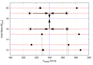
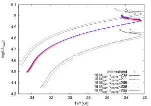
STARMAKER simulates a prescribed number of stars, with initial mass (), initial rotational velocity (), and age () drawn from the corresponding distribution function (IMF, initial distribution of rotational velocities, and SFH). For a given initial triplet (, , and ), four evolutionary sequences from the grid of stellar evolution calculations are selected, and then used to interpolate the stellar parameters using a 3D linear interpolation algorithm.
For a given and , the interpolation routine first determines the two closest masses above and below in the model grid. Then, for each of the two, it chooses the two models with closest to the required value (Fig. 1). We found that the algorithm works best when the four selected model sequences form two pairs with equal masses. For example, to interpolate an 18 model, two 16 and two 19 models enter the interpolation. An interpolated track is show in Fig. 1 (bottom). Initial masses and initial velocities may be irregularly spaced in the model grid, but for every new mass introduced into the model grid, models of several rotational velocities are required to cover the -parameter space considered in the simulation.
As indicated by the arrows in Fig. 1, we first interpolate models of equal mass to obtain models with the desired initial velocity, and then we interpolate in mass. We tested our result by changing the interpolation order, and found no significant differences. Adopting the nearest neighbors for interpolation , i.e the smallest distance , would often result in selecting models of three or four different initial masses due to the domination of the velocity term in the distance equation (models marked by a triangle in Fig. 1). We found this could lead to unsatisfactory results.
Stars with different initial masses and rotation velocities achieve different main-sequence lifetimes. To facilitate the interpolation in time, we use the fractional main-sequence lifetime as the interpolation variable. For all models in the grid their MS-lifetimes have been tabulated so that, for any pair (, ), the expected MS-lifetime can be interpolated. To ensure a smooth behavior of isochrones in the HR diagram we fit the MS-lifetime for each initial mass as function of with a polynomial, and add a linear fit for masses where quasi-chemically homogeneous evolution is achieved for the highest rotational velocities (Fig. 2). The increase in the MS-lifetime for higher rotational velocity is due to rotational mixing of hydrogen into the convective core. This effect saturates when the rotational mixing timescale becomes shorter than the main sequence timescale. At this point the star becomes quasi-chemically homogeneous (e.g. Maeder 1987; Yoon & Langer 2005), implying its interior is well mixed and the star can burn basically all the fuel it contains.
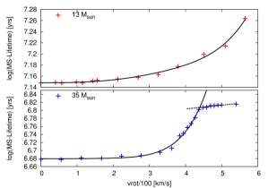
Any observable can now be interpolated using the four model sequences used for interpolation (Fig. 1). As each model sequence is highly resolved in time (with several thousand time steps for the main sequence evolution), the interpolation error in time is negligible.
3.2 Initial distribution functions
In our population synthesis we draw the three initial parameters (, , and ), from the initial distribution functions, which are discussed below. We also adopt an inclination angle for the star, assuming random orientation in space.
3.2.1 Star formation history
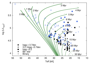
We have used our population synthesis code to generate isochrones for non-rotating stars with ages between 0 and 30 Myrs from our stellar evolution grid (see Paper I, ). In order to evaluate the appropriate star formation history for our population synthesis model, we compare those isochrones with the distribution of the stars of our observational sample in Fig. 3.
The N11 region (blue symbols) contains a number of stars with ages younger than 5 Myr. These are primarily the massive O-type stars, associated with the recent star formation in, e.g., LH 10. Both fields contain older populations with ages in the range of 5 to 25 Myr, and with no obvious preference for a particular age (Fig. 3). Given that we do not include the O-type stars in our analysis (see Sec. 3.3), we therefore adopt continuous star formation as a good approximation of the observed lower-mass population in our population synthesis models.
3.2.2 Initial mass function
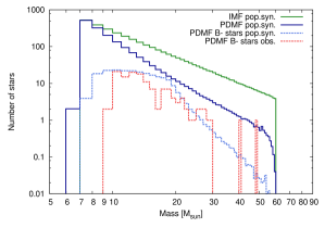
As input for our population synthesis we adopted a Salpeter (1955) IMF. The masses are randomly picked from the IMF in the range between 7 and 60 , and the result is plotted in Fig. 4 (green, solid line). The present day mass function (PDMF) of our population synthesis simulation is also plotted (blue, solid line). It contains only main sequence stars and is calculated assuming continuous star formation. A comparison between the IMF and PDMF shows that mass loss has populated the 6 -bin and that the (negative) slope of the PDMF has increased. The latter is an evolutionary effect: the most massive stars evolve more quickly and once they leave the MS they are removed from the population. At the high mass end the PDMF gets incomplete as mass loss shifts stars to lower mass bins and we do not have stars initially more massive than 60 in our simulation.
To test if our assumptions on the IMF and the SFH are reasonable, we construct the PDMF of the stars that would pass all observational selection effects in our population synthesis simulation (see Sec. 3.3 below). This distribution corresponds to the light-blue dashed line in Fig. 4, and is compared to the PDMF of the stars in our sample (red line). A plateau at lower masses develops, since many low mass stars are too faint to be included in the observational sample. At higher masses, the slope steepens further, since the hot O-type stars drop out of the sample (see Sec. 3.3). This can be directly compared to the observed sample PDMF, shown as a red, dashed line in Fig. 4. Keeping in mind the low number statistics in the observed sample, it appears that below 30 the two curves have approximately the same shape, thus supporting the assumptions made for the simulation.
The lowest mass stars in the observed sample are 9 while the lowest mass stars in the simulation are 7 . This is confirmed in Fig. 6, where no stars are observed at the lowest masses. This could imply that the SFH is limited to 25 Myrs, or — perhaps more likely — that the sample selection concentrated on the brighter stars in the field. This discrepancy between our model and the observational sample might introduce an error in our analysis. However, the error caused in the population numbers of the different regions of the Hunter-diagram by including stars older than 25 Myrs in the simulation is on the order of 1%. We discuss this in more detail in Sec. 4.1.
3.2.3 Initial velocity distribution
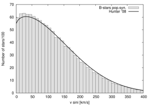
Hunter et al. (2008b) fitted the observed rotational velocity distribution of the LMC sample with a Gaussian function, excluding radial velocity variables, supergiants and stars above 25 . This mass threshold was used to avoid effects from mass loss induced spin-down on the velocity distribution (see Fig. 5). As such, all but the seven lowest mass O-type stars were not included in determining the velocity distribution. Be-stars below the mass threshold are included into the fit to the velocity distribution. As discussed byHunter et al. (2009b), the width of this function given by Hunter et al. (2008b) is too small and needs to be corrected by a factor . Taking this into account, our ZAMS rotational velocities are selected randomly from the Gaussian function given in Eq. 1 (using km/skm/s), which has been truncated at zero km/s and renormalized (see Hunter et al. 2008b).
| (1) |
By using this function for our population synthesis, we assume that it is representative of the distribution function of the initial rotational velocities. This is justified when the stars rotate close to solid body rotation, which is ensured by including magnetic fields in our models. Also, due to the low mass loss rates for the bulk of the stars in the sample, our models show little change of the rotational velocity over the main sequence evolution. To test this assumption, we have constructed a histogram of the present day projected rotational velocity distribution (PDVD) for the B-type stars from our population synthesis (gray bars in Fig. 5). Comparing this for the initial projected rotational velocity distribution (black line) from Hunter et al. (2008b), our simulation predicts only slightly more slow rotators than the input function, but also slightly fewer fast rotators around 200 km/s. The overall shape at lower rotational velocities is preserved in our simulated data. Overall, the observed B-type star velocity distribution seems to be a good approximation to the initial velocity distribution of our population synthesis simulation.
3.3 Selection effects
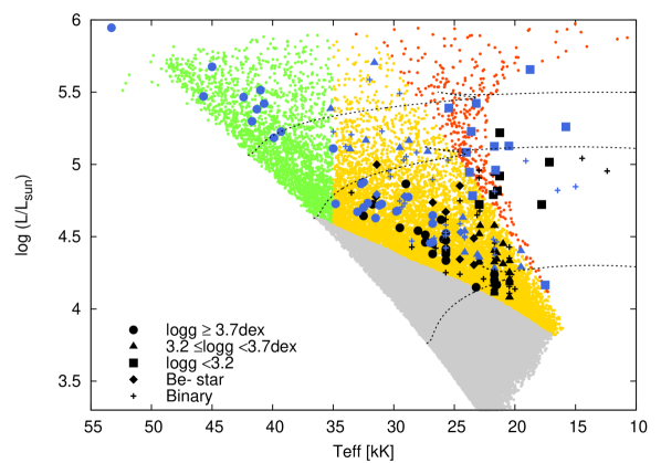
The VLT-FLAMES survey was designed to contain a largely unbiased sample of O- and B-type stars. However, owing to both observational and analytical constraints, there are a number of selection effects present in the final Hunter et al. (2008b) sample (see 2), which we attempt to include in our simulation. Specific affected regions in the H-R diagram are highlighted in Fig. 6.
3.3.1 Magnitude limit
Our LMC sample is magnitude limited, to ensure sufficient signal-to-noise in each observed spectrum, with about for the faintest star. While the limit is not exactly the same in N11 and NGC2004, the limits in each are not significantly different and hence it is reasonable to model these together. In our simulation, we therefore remove all simulated stars that are fainter than this threshold from our simulation, with this region marked in gray in Fig. 6. Magnitudes for the simulated stars have been calculated using:
| (2) |
| (3) |
where is the absolute bolometric magnitude of the simulated star. Observational parameters are adopted such that they are consistent with those used by Hunter et al. (2008b) for NGC 2004, i.e., distance modulus () 18.56m, 0.09m, and a ratio of total-to-selective extinction 3.1. Bolometric corrections (BC) for have been adopted from Balona (1994), and for from Vacca et al. (1996).
3.3.2 Exclusion of O-type stars
The dominant nitrogen lines in O-type stars are those from N iii. However, this ion is notoriously difficult to model in non local thermodynamic equilibrium due to the need to include di-electronic recombination channels. To date, no large studies of nitrogen abundances in O-type stars are available, although He abundances were studied by Mokiem et al. (2006, 2007). Due to the lack of nitrogen abundances for stars hotter than 35 kK we exclude such hot stars from the simulation (green group in Fig. 6), corresponding to spectral types earlier than O9.
3.3.3 Exclusion of low gravity objects
The bulk of the stars have masses in the range of 10 to 20 . Paper I argues that the surface gravity at the end of the main sequence evolution for these objects is (see also Hunter et al. 2008b). While there are some observed stars with lower , their nature is unclear (Vink et al. 2010). We therefore exclude post-MS objects, by rejecting all simulated stars with gravities below 3.2 dex (red regime in Fig. 6). Note that this implies that we also reject the final part of the main sequence evolution of stars with masses above , since the applied overshooting leads to an extension of the main sequence to lower gravities for these objects. We chose to do this because we favor a well defined selection criterion and because the most massive objects have only a low impact on our statistics. Most of the observed stars rejected are luminosity class I supergiants, but this group also contains three class II and two class III objects.
3.3.4 Exclusion of Be stars
Hunter et al. (2009a) did not derive nitrogen abundances for most of the observed Be-type stars (the purple group in Fig. 13). For consistency, we excluded a fraction of the most rapid rotators in our simulation. As the mechanism that produces the Be-phenomenon is still being discussed, it is difficult to define a clear criterion to identify simulated stars as Be stars. The Be mechanism appears to be linked with fast rotation and pulsations (e.g. Cranmer 2005). Commonly quoted required fractions of critical rotation for the occurrence of the Be phenomenon are 70-80% (Porter & Rivinius 2003), though values as low as 40% (Cranmer 2005) are also derived. Martayan et al. (2008) finds = 85% in the LMC, and Townsend et al. (2004) argue that Be-stars might actually rotate as fast as 95% of the breakup velocity, since the line broadening due to rotation becomes insensitive to gravity darkening at high rotational velocities.
The fraction of Be/(B+Be) in the observed sample is 13.5%. We can define a theoretical Be fraction within the limits of the yellow region of Fig. 6 by dividing the number of stars rotating faster than a specified fraction of break-up rotation by the number of all stars in that region. To match this fraction with the observed one in our sample would require a velocity limit of 55% of the break-up velocity. This number seems too low. As clearly more effects than fast rotation are involved in producing Be stars, we decided to not try to reproduce their number in the population synthesis. In an attempt to simulate the effect of the exclusion of Be-stars from the sample, we chose a more conservative limit and excluded stars with a rotational velocity higher than 90% of their breakup velocity in our simulations. This corresponds to 1.6% of all stars in the yellow region of Fig. 6.
In summary, we are unable to reproduce the fraction of observed Be-stars using our cut-off of 90% of breakup velocity. However as we only exclude a small minority of stars from the simulation, we do not expect that this will be a significant source of error.
3.4 Stellar evolution models

We calculated a grid of 284 stellar evolution models past core hydrogen exhaustion using a one-dimensional hydrodynamic stellar evolution code, that includes the physics of differential rotation and magnetic fields as described in Paper I; see also Yoon et al. (2006) and de Mink et al. (2009). The grid spans initial masses of 5–60 and rotational velocities () of 0–600 km/s, as shown in Fig. 7. The grid is somewhat irregular in rotational velocity since we initialize our models as rigid rotators in a chemically homogeneous state of thermal equilibrium. The subsequent adjustments to achieve CN-equilibrium in the core alter the stellar structure on a thermal time scale and lead to a somewhat different surface rotation rate, which thereafter changes only on the nuclear time scale, and which we designate as .
The effect of the centrifugal force on the stellar structure is considered following Endal & Sofia (1976). We consider the transport of angular momentum and chemical elements due to various rotationally induced hydrodynamic instabilities, which include the Eddington-Sweet circulation, the dynamical and secular shear instability, and the Goldreich-Schubert-Fricke instability (Heger et al. 2000). The transport of angular momentum by the Spruit-Tayler dynamo (Spruit 2002) is also implemented. Angular momentum transport and chemical mixing is approximated as a diffusive process.
Convection is treated by the mixing length theory assuming a mixing-length parameter of = 1.5. We follow Langer (1991) for semi-convection, for which rather fast mixing is assumed, with a semi-convection efficiency parameter of =1. We consider convective overshooting using an overshooting parameter of . This value results from our new calibration using the observed drop that is found in our data when we plot against the surface gravity (see Paper I, ) for more details). The rotational mixing efficiency has been calibrated such that the trends in nitrogen of our sample are reproduced well. This leads to adopting = 0.0228, which is the ratio of the turbulent viscosity to the diffusion coefficient (see Heger et al. 2000).
We use the recipe of Vink et al. (2000, 2001) for mass loss via stellar winds from O- and B-type stars. To account for the effects of helium enrichment on the stellar wind, we follow the approach of Yoon et al. (2006) (see Paper I for details).
3.4.1 Initial chemical composition
We choose an LMC mixture for the initial chemical composition of our models (Table 1). CNO abundances are taken from results for H ii regions (Kurt & Dufour 1998). Mg and Si measurements for B-type stars from Hunter et al. (2008b) and B-supergiants of Trundle et al. (2007) are, on average, 0.37 dex lower than the solar values of Asplund et al. (2005). Therefore, we have scaled all other elements from Asplund et al. (2005) by -0.4 dex and adopted the average values of Mg and Si from Hunter et al. (2007) and Trundle et al. (2007) for our stellar models. The resulting metallicity of this mixture is . We have adopted the OPAL opacity tables (Iglesias & Rogers 1996), for which we use the Fe abundance to interpolate between tables of different metallicities.
We have adopted the helium mass fraction using the primordial helium abundance ( 0.2477) from Peimbert et al. (2007). Assuming the helium abundance to be a linear function of the metallicity and fixing it to 0.28 at solar metallicity (Grevesse et al. 1996) results in a value of 0.2562 for our LMC models.
| C | 7.75 | Mg | 7.05 | X | 0.7391 |
|---|---|---|---|---|---|
| N | 6.90 | Si | 7.20 | Y | 0.2562 |
| O | 8.35 | Fe | 7.05 | Z | 0.0047 |
More details on the calibration and choice of the chemical composition for the full
evolutionary model grid, which also includes models for Galactic and
SMC stars, are presented in Paper I.
3.5 Effects of rotational mixing
In our models, the strong transport of angular momentum due to the
Spruit-Tayler dynamo keeps the star rotating almost rigidly on the main
sequence. As a consequence, the shear instability – which is
important for non-magnetic models (Heger et al. 2000; Maeder 2000) –
is less efficient than the Eddington-Sweet circulation in our models.
The surface abundances of stars can change due to rotational mixing on the main
sequence but not all elements are equally well suited for tracing such
mixing. While helium is produced in large amounts in the core, the models for
moderate rotational velocity show only small enhancements of helium at the
surface. This is because the chemical stratification built up by hydrogen
burning between the helium enriched core and the hydrogen-rich envelope
effectively hinders chemical mixing across the boundary. Only the fastest
rotating models ( 350 ) become significantly helium enriched at
the surface, and some of them even follow the quasi-chemically homogeneous
evolution if rotational mixing operates faster than hydrogen burning
(Yoon et al. 2006). Additionally, helium is already abundant at the stellar surface
initially, and the expected enhancement relative to the initial
helium abundance is typically small.
Nitrogen, however, can be considerably enhanced at the stellar surface on the MS, even in relatively slow rotators. At the same time, carbon is depleted, but with a smaller relative change than nitrogen, and oxygen remains almost constant. This can be understood in the following way. At the onset of the CNO-cycle, there is a short phase of the CN-cycle in which most of the carbon is transformed to nitrogen. During this phase, hardly any helium is produced, and the mean molecular weight gradient at the outer edge of the core remains small. Therefore, nitrogen produced by the CN-cycle can be efficiently transported into the layers above the convective core. Once the mean molecular weight gradient increases due to helium production, such mixing becomes much slower. As mixing throughout the radiative envelope — i.e. above the major mean molecular weight barrier produced by hydrogen burning — continues during the main sequence evolution, the surface becomes gradually enriched with nitrogen. As the nitrogen abundance at the surface of early B type stars can be measured from optical spectroscopy, nitrogen is one of the best tracers for rotationally-induced chemical mixing.
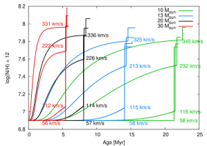
In Fig. 8 we show the surface nitrogen abundance as a function of time for a selection of models from our grid. As the nitrogen enrichment during the main sequence evolution is a monotonic function of time, nitrogen might be used as an age indicator for stars with known initial stellar parameters. In our models, the nitrogen abundance achieved at the end of core hydrogen burning is higher for higher initial rotation velocities, as the Eddington-Sweet circulation operates at a higher flow velocity for faster rotation (Yoon et al. 2006). At the same time, at fixed initial rotation velocity, the maximum nitrogen abundance increases only slightly with initial mass in the range of 10 to 20 , but it becomes more sensitive at masses above 30 . When hydrogen burning stops, the core contracts and the envelope expands and eventually becomes convective, leading to a further dredge-up of nitrogen and a sharp increase of the nitrogen surface abundance as shown in Fig. 8.
The abundances of other elements also show variations due to rotational mixing. Sodium is enhanced due to proton captures in the NaNe-cycle, but it is difficult to determine observationally as its lines are weak in this mass range and they are contaminated by interstellar absorption. Boron is strongly depleted, because it is destroyed as it is mixed from the relatively cool outer layers into hotter inner layers (see Paper I, ), but its spectral lines are weak due to the low initial abundances. Carbon depletion can also be observed in the optical, but it cannot be measured as accurately as nitrogen due to NLTE effects (Hunter et al. 2008b). Fluorine and aluminum are also affected. A full account of this is given in Paper I; in what follows we concentrate on the nitrogen abundances.
4 Results
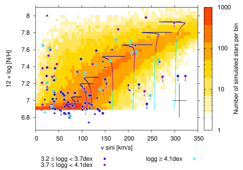
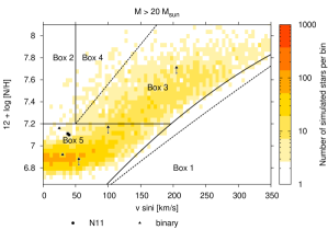
To investigate the role of rotational mixing in massive stars, Fig. 9 shows projected equatorial rotational velocities versus nitrogen abundance (hereafter the Hunter plot). The figure contains both observations and theoretical predictions. The observational data includes all stars from our LMC sample for which nitrogen abundances are available (see Sec. 2). Radial velocity variables are marked by triangles, while stars with no detected variations are represented with circles. The color coding of the symbol indicates the surface gravity of each object as shown.
The simulation considered 1.5 million stars with initial masses between 7 and 60 . Only those that remained in the main sequence can be compared to the observational sample. These are plotted in Fig. 9. About 45.7% of initial sample have left the main sequence, whilst another 46.3% were excluded due to selection criteria based on magnitude, temperature (spectral type) and surface gravity (see Sec. 3.3). The remaining sample contains 120 728 stars.
The most important rejection criterion is the magnitude cutoff, but the age of the simulated star also has a considerable effect. This is easily understood considering that the maximum age of 35 Myr in our SFH corresponds to the MS-lifetime of an 8 model. As the MS-lifetime decreases rapidly with increasing initial mass (see Fig. 8), the chance that a simulated star is assigned an age greater than its MS-lifetime becomes significant.
The magnitude cutoff eliminates a large number of simulated stars because the IMF favors lower masses. For instance, models with less than 20 are too faint to be observed for most of their MS-lifetime. A 12 star spends 72% of its MS-lifetime below the magnitude limit, while a 15 star is not observable for 35% of its MS-lifetime.
The simulated data have been grouped into km/s bins to generate a density plot. The color coding represents the number of stars in the bin (see the color bar on the right in Fig. 9). We also show evolutionary tracks of 13 for comparison. For these tracks the surface gravity is indicated with the same color coding as for the observational data.
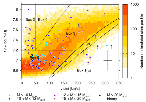
Fig. 10 shows the same population synthesis simulation as Fig. 9, but we have added a random Gaussian error with to the predicted nitrogen abundances. This error is characteristic of the spread in the nitrogen abundance determinations of the unenriched stars. Note that it is smaller than the mean nitrogen error of the entire sample (0.3–0.4 dex; Hunter et al. 2007, 2008b), which is represented by the cross in the lower right corner of Fig. 9 and 10. We did not include an error for the predicted values as the observational values should be reasonably secure. The color coding of the observational data in Fig. 10 represents their estimated evolutionary mass.
We have divided the diagram into five regimes:
-
Box 1(ab) is a region of the diagram at high which is predicted to be almost empty. The full line defining box 1(ab) gives the locus where the number of simulated stars per pixel is , while this number is for the dashed line defining Box 1b.
-
Box 2 is a region of the diagram where very few stars are predicted, but where a group of enhanced, slowly rotating stars are observed. This group of stars was already described by Hunter et al. (2009a), and will be discussed further below.
-
Box 3 encloses the stars in our simulation which have a clear signal of nitrogen enhancement due to rotational mixing.
-
Box 4 is a region where neither stars are observed, nor a significant number of them is predicted.
-
Box 5 is the region of the diagram where the un-enriched stars are located. The initial nitrogen abundance is about 6.9 with a typical spread of about 0.2 dex. We chose the upper boundary of 7.2 such that the probability of observed stars found above this line to be truly enriched is large.
| observed | modeled | |||||
|---|---|---|---|---|---|---|
| all | excl. UL | |||||
| % | # | % | # | % | # | |
| Box 1ab | 14.0 | 15 | 7.4 | 6 | ||
| Box 1a | 5.6 | 9 | 0 | 0 | ||
| Box 1b | 8.4 | 6 | 7.4 | 6 | ||
| Box 2 | 15.0 | 16 | 19.8 | 16 | ||
| Box 3 | 17.8 | 19 | 13.6 | 11 | ||
| Box 4 | — | — | ||||
| Box 5 | 53.3 | 57 | 59.3 | 48 | ||
| Total | 107 | 81 | ||||
In Table 2 we present the absolute and relative number of stars populating each box in both the observations and simulations. For the observations we present statistics including and excluding objects for which only an upper limit to the nitrogen abundance was established. A downward revision of the upper limits might reduce the number of observed stars in Box 3, while that in Boxes 5 and 1 might increase. For all stars in Box 1a we only have upper limits, but their presence in this box is not affected by this. Unless otherwise stated, the numbers quoted in the discussion below include the stars with upper limits to their nitrogen abundances.
We find 53.3% of the total observed sample to be in Box 5, containing the unenriched stars which do not rotate rapidly. This is in good agreement with the theoretical prediction of 55.9%. Due to the large number of stars in this region, this agreement is not affected by stars with upper limits on their nitrogen abundance. Most of the stars in this box are expected to have a relatively low mass, and in an advanced phase of core hydrogen burning such that they have become sufficiently bright in the optical to be above the magnitude cutoff. Indeed the observed stars with 10 accumulate in Box 5 and appear to have mainly surface gravities of less than 3.7.
We note that a more efficient mixing would reduce the predicted number of stars in Box 5. However, the mixing efficiency is calibrated to best represent the correlation between nitrogen abundance and (see above). The fact that after such a calibration the number of non enriched stars predicted in Box 5 is in very good agreement with the observations supports the theory of rotational mixing.
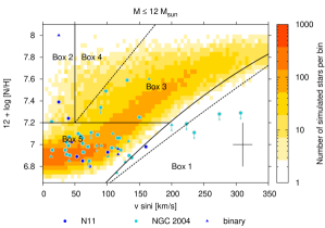
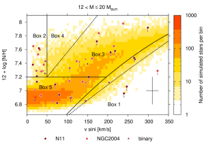
Box 3, containing the stars of our simulation which show rotationally induced nitrogen enhancement, is predicted to contain 35.7% of our sample. However only 17.8% of the observed sample is found in this region. Hence we predict approximately twice as many stars to be enriched as are actually observed. Subtracting the stars for which we have only upper limits leaves only 13.6% of the sample stars in Box 3, increasing the discrepancy between theory and observations to almost a factor of three. On the other hand, Fig. 11 shows that more observed stars in Box 3 are found in the 12…20 bin compared to the lower mass bin (), while our models predict similar (absolute) numbers for both mass bins. This may indicate that subdividing our sample into too small subsamples results in a loss of statistical significance.
While this may show that analyzing subsamples may lead to effects of small number statistics, it also shows that the overall discrepancy in the predicted and observed number of stars in Box 3 may not be very significant.
Box 2 contains a group of apparently slowly rotating but nitrogen enhanced stars. Theoretical models of rotating single stars predict such enhancements only for fast intrinsic rotation (km/s). Note that all the observed targets in Box 2 cannot be rapid rotators seen nearly pole on. Indeed our simulations (which assume random inclination angles) predict that only 1.2% of the sample (corresponding to one star) would be found in this region. Observationally 16 stars comprising 15% of the sample lie in Box 2. Therefore the projection effect cannot populate this part of the diagram. This statement is enforced by the fact that no stars are observed in Box 4, which — if the projection effect were to explain the large number of stars in Box 2 — should contain more stars than found in Box 2. We conclude that the vast majority of stars in Box 2 are intrinsically slow rotators and their high nitrogen abundance is not explained by our models. The nitrogen enhanced stars in Box 2 appear to have higher masses and to be less evolved. There are no stars with 10 in this group, even though this is one of the most populated mass bins in the observed sample. With the exception of five stars (of which one is a binary) surface gravities in this group are larger than 3.7 dex. A comparison with the evolutionary tracks in Fig. 9 indicates that most stars of this box are in an intermediate or evolved stage of their MS-evolution. The large number of stars found in Box 2 is not predicted by the theory of rotational mixing in single stars with an overpopulation of observed targets by more than a factor of ten with that predicted.
Box 1(a+b) contains a group of 15 fast rotating but unenriched stars (14% of the observed sample). We predict a factor of 3 less stars (4.6%) in this box, with most of them expected to be in Box 1b, i.e. very close to Boxes 3 and 5. In particular the area where the six observed stars in Box 1a are found is predicted to be empty. This prediction is largely due to the adopted observational selection effects, but to a small extent also due to the fast nitrogen enrichment of rapidly rotating stars (Fig. 8). Most of the simulated targets populating the diagram started their evolution below the magnitude cutoff. Those which were rapidly rotating have sufficient time (before passing the magnitude limit) to enhance their surface nitrogen abundance so significantly that once they appear in the diagram they show up in Box 3. In Box 1(a or a+b), there does not seem to be a preference for high surface gravities and low masses as suggested by Maeder et al. (2009). The six objects in Box 1a have masses in the range of , which is a typical spread for the sample. Their average mass is 12 which is similar to the average for all the stars for which nitrogen abundances have been determined of 13.6 . Additionally the stars cover a range of ages. As the stars in Box 1b have upper limits to their nitrogen abundances, some of them could actually lie in Box 1a, increasing the discrepancy with prediction. In summary the existence of a significant number of targets in Box 1a cannot be reconciled with the prediction of rotational mixing for single stars that this area should contain effectively no objects.
Fig. 11 indicates that whilst the population of Box 1b is strongly mass dependent, that dependency is less pronounced for Box 1a. The top panel shows simulation and data with . The models of 12 spend about 70% of their MS at luminosities below the magnitude limit. When they finally become bright enough, they are already so enriched that they show up in Box 3. Only for models of intermediate mass, as shown in the middle panel (12–20 ), does the interplay between the selection effects and the mixing-timescale allow stars to populate Box 1. Using an even finer mass binning, we find that Box 1a is actually only populated by stars in the mass range 12–15 , while Box 1b contains models in the mass range 12–20 . The bottom panel shows models and observed stars more massive than 20 . In both cases Box 1 remains empty. Models of 20 or more are above the magnitude limit all time, but they have effective temperatures above 35 000 K during their early main sequence evolution, such that the fast rotators, once they have become cool enough to appear in our simulation data, have already achieved a significant nitrogen enrichment.
4.1 Model uncertainties
Before we focus on the possible evolutionary implication of our findings, we first discuss the significance of the results summarized in Table 2 which are obtained from our population synthesis. The discrepancy between observation and prediction is very large for both Boxes 1 and 2. In contrast, it is smaller for Box 3, being only a factor of approximately two. Hence in discussing our uncertainties, we will focus on how they might affect our simulation of the fractional population of this Box.
These numbers are subject to various uncertainties: i) the mixing efficiency in the stellar models, ii) the initial velocity distribution, mass function and star formation history, iii) the observational biases, and iv) exclusion of unsuitable stars.
4.1.1 Mixing efficiency
The calibration of the mixing efficiency is described in detail in Paper I. The models in our stellar evolution grid are calculated with a mixing efficiency parameter of (see Sec. 3.4). The impact of a larger mixing parameter is that a larger maximum nitrogen enhancement is achieved for a given initial rotation rate. Therefore, the general trend of nitrogen enhancement versus would be shifted to lower rotation velocities and larger nitrogen abundances. In Fig. 9, the evolutionary tracks of our 13 models show an unaffected nitrogen abundance for km/s within the observational error, and a peak value of 7.9 is obtained at km/s. This behavior does reflect the general trend of the observed stars in Boxes 5 and 3 quite well: the maximum observed nitrogen abundance, the slope of the nitrogen versus -relation, and the foot-point at km/s are all matched well. We thus believe that the calibration of the mixing efficiency of our models does not contribute significantly to the observed discrepancy.
4.1.2 Input distribution functions
The adopted distribution of initial rotational velocities has been discussed in Sec. 3.2.3. In order to assess the sensitivity of the predictions on the distribution of initial rotational velocities, we investigated the effect of a broader (km/s) and narrower (km/s) width of the underlying Gaussian. A variation of km/s is consistent with the errors given in Dufton et al. (2006) on the fit to the projected rotational velocity distribution. The relative changes are given as errors on the theoretical percentages in Table 2. While we find that the numbers predicted for most boxes do not change significantly, the narrower velocity distribution leading to fewer rapid rotators, shifts about 6% of all modeled stars from Box 3 to Box 5. This reduces the discrepancy for Box 3 (35.7% predicted vs. 17.8% observed) to below a factor of two (29.8% predicted vs. 17.8% observed), but it cannot eliminate it.
The initial mass function is assumed to be Salpeter (; see Sec. 3.2.2). Given the apparent universal nature of this distribution in the mass range from 10–60 (Chabrier 2003; Kroupa 2001), and given the good agreement between the observed and simulated mass functions (see Fig. 4) we believe that this is unlikely to be a significant source of error.
As discussed in Sec. 3.2.1, we have assumed continuous star formation in our population synthesis model. Clearly, the star formation history may influence the distribution of stars in Fig. 10. For instance, a young co-coeval population will cause the fraction of predicted stars in Box 5 to increase, at the expense of the number of stars in Box 3. However, as Fig. 3 appears largely consistent with our assumption of continuous star formation, we do not expect a significant error due to this assumption. We have investigated the case where star formation stopped after 25 Myr (as suggested in Sec 3.2) instead of continuing for 35 Myr. The stars that are older than 25 Myr are mainly to be found in Boxes 3 and 5. If we exclude these stars, the number of stars in Boxes 3 and 5 change by about 1%, and by much less in the other boxes.
4.1.3 Observational biases
While we accounted for the observational biases in our population synthesis model, some error may be associated with this. Most relevant in this respect may be the magnitude cut-off applied in the VLT-FLAMES Survey. While Fig. 6 shows that indeed no observed stars fainter than our adopted magnitude cut-off are found in the sample, there may be a slight deficit of observed stars near the magnitude cut-off, especially at masses below . As these stars would be nearly at the end of their main sequence evolution, the ratio of enriched to unenriched stars amongst them would be greater than average. However, limiting the population synthesis to stars above 9 has a very similar effect as limiting the star formation history to 25 Myrs (discussed above), since the main-sequence lifetime of a non-rotating 9 model is about 25 Myrs. It changes the number of stars in Box 3 and 5 only by less than one percent. The main-sequence lifetime of a non-rotating 9 model is about 25 Myrs.
Binary stars are slightly brighter than single stars of a mass or brightness equal to the binary primary. Therefore, some binaries with primaries which would not pass the magnitude limit by themselves might, through the additional light of their companion. A test population simulation where we assumed all stars to consist of binary stars with identical companions convinced us that this effect does not significantly affect any results described below.
For very rapid rotators, the observed brightness and gravity may also depend on the inclination angle due to the latitudinal dependence of gravity darkening. However, the observed and the modeled number of very rapid rotators is so small that this effect is negligible here (see also Hunter et al. 2009a).
4.1.4 Removal of unsuitable stars
In our population synthesis simulation, we have only included single stars computed with a single set of physics assumptions. In reality however, different physical situations may occur. For example, many massive stars are known to have a close binary companion (e.g. Sana et al. 2009) which will modify the evolution during core hydrogen burning. Other massive stars are clearly affected by internal magnetic fields (e.g. Wade et al. 2006). It remains unclear wether the magnetic fields used in our evolutionary models for angular momentum transport describe those detected in massive stars. Our population synthesis model is therefore only representative of at most a certain fraction of the observed stars.
In order to assess the potential consequences for our conclusions concerning the number of stars in Box 3, let us first assume that the stars in Boxes 1 and 2, which cannot be explained well by our model anyway, need to be discarded as “unsuitable” for a comparison with our model. This would reduce the total number of stars to be compared with from 107 to 76, and then render the fraction of observed stars in Box 3 to 25% (rather than 17.8%), which is closer to the predicted fraction of 35.7%.
However, the fraction of observed stars which is “unsuitable” for a comparison with our model may be greater; let us assume it is as high as 50%. As the observed stars in Box 3 agree well with the physics of rotational mixing, let us further assume that none of the 50 or so observed stars to be disregarded would lie in Box 3. Again, we would assume that the observed stars in Boxes 1 and 2 should be disregarded. However, about 20 stars need to be disregarded also from Box 5. For example, this could be fast rotators which cannot mix because of strong internal magnetic fields. With such assumptions, we had 37 “suitable” stars left in Box 5, and 19 in Box 3. The latter number corresponds to 33% of the reduced sample, which then is close to the predicted fraction of 35.7%. While the assumption that we can describe only half of the stars in the observed sample may be extreme, this case cannot be ruled out, and it serves as an example of the difficulty in defining a robust observational sample.
4.1.5 Stochastic effects
Here, we assess the spread in the number of stars obtained for each box in Fig. 10 if only 107 stars are drawn randomly from the simulated population. This is equivalent to the following experiment. A pot contains N=120 728 balls, equivalent to the number of simulated stars in Fig. 10. The balls in the pot have the colors cc5. The number of balls in the pot with color ci is equal to the number of simulated stars in Box i, for . We draw n=107 balls from this pot, without taking the order into account in which they are drawn. Because of the large number of balls in the pot, the probability to pick a certain color can be approximated as constant, i.e. as the number of balls of color ci divided by the total number of balls N. This approximation is valid as long the number of balls of color ci is much larger than the number of balls drawn from the pot.
When the experiment is repeated many times, the result is multinominally distributed(Papoulis 1984, p. 75). The expectation values for the number balls drawn from each color and its standard deviation can be calculated by:
| (4) | ||||
| (5) |
The expectation values given in Table 3 agree with the percentages found in Table 2. The standard deviation indicates a rather small spread, which cannot cause the discrepancy between observation and simulation discussed above. This is true in particular for the ratio of the number of stars from Box 3 and Box 5.
| [#] | [%] | |
|---|---|---|
| Box 1 | 4.9 2.2 | 4.6 2.0 |
| Box 2 | 1.3 1.1 | 1.2 1.0 |
| Box 3 | 38.2 5.0 | 35.7 4.6 |
| Box 4 | 2.8 1.6 | 2.6 1.5 |
| Box 5 | 59.8 5.1 | 55.9 4.8 |
4.1.6 Overall assessment
We have shown above that the discrepancy of a factor of two in the predicted and observed fraction of stars in Box 3 is not sufficient to rule out rotational mixing for this subsample. Our theoretical mixing calibration, the adopted star formation history, and initial distribution functions for mass and rotational velocity apparently induce little uncertainty. However, the adopted magnitude cut-off and in particular the possibility of applying different physical situations to main sequence stars than assumed in our model allows for a modification of the fractions of stars in Boxes 3 and 5 which may bring theory and observations into agreement.
On the other hand, the possible agreement of the predicted distribution of stars in Boxes 3 and 5 is not sufficient to verify the theory of rotational mixing. This will be discussed further when predictions of massive close binary evolution are included in our considerations, in the next section.
5 Discussion
From the previous section, we conclude that overall, the agreement between the population synthesis model and the observed sample is rather poor. While the model predicts stars to be confined to Boxes 5 and 3, the observed stars are much more wide spread. Quantitatively, only in Box 5 is the number of observed stars in good agreement with the predictions. While the stars in Box 3 at least qualitatively agree with the population synthesis model, the stars in Box 1 and Box 2 are completely unexpected and cannot be explained by the model. Before any further conclusion, it is thus worthwhile to consider physical and evolutionary processes which could populate Boxes 1 and 2, as those might have effects on Boxes 3 and 4.
5.1 Close binary evolution
Though our model assumption is that the diagram is populated only by single stars, it is well known that a significant fraction of stars is part of a binary system (e.g., Mason et al. 2009), with a binary fraction of 0.5 or more found in young star clusters (e.g., Sana et al. 2008, 2009; Bosch et al. 2009), and with a period distribution such that many of them will interact (Sana & Le Bouquin 2010). We emphasize that strong binary interaction (i.e., mass transfer or merging) will often lead to a system that is either a single star or which shows insignificant radial velocity variations. Most observed radial velocity variables in the VLT-FLAMES Survey will likely be pre-interaction systems and thus well suited for comparison with single star evolution. The apparent binary fraction in our various observational subsamples thus give no direct clue to the importance of strong binary interaction for the subsample.
In close binaries, the primary star may fill its Roche lobe during the main sequence evolution. This results in the removal of the stellar envelope of the primary star, which is transformed into a (mostly unobservable) helium star. If the entire envelope is added to the companion, the surface nitrogen abundance of this star will increase by a factor of 3 to 5, even when rotational mixing is not taken into account (cf., Fig. 9 in Langer et al. 2008) as in the accretion process the envelope material is well mixed. Subsequent rotational mixing of the mass gainer may enhance the surface nitrogen abundance further on the thermonuclear timescale (cf., Fig. 10 in Langer et al. 2008). If only a small fraction of the material is accreted, the result is no or only a mild N enrichment. During the accretion process not only mass but also angular momentum is transferred to the companion, and it has been found that the accretion of only about 10% of the stellar mass is able to spin-up the star significantly (Packet 1981; Langer et al. 2008).
Therefore, conservative and moderately non-conservative mass transfer would tend to populate the upper right corner in Fig. 10 (Box 3), while highly non-conservative mass transfer (e.g., Petrovic et al. 2005) is likely to move stars to the lower right corner (Box 1) (Langer et al. 2008). Binary interaction leading to a merger is also expected to result in fast rotating objects, likely populating Box 1 or Box3̇. Binary evolution is also able to populate Box 2, as post-mass transfer systems may remain so tight that the tidal interaction can spin down the accretion star (Langer et al. 2008).
While quantitative statements requires binary population synthesis models which include a methodology for non-conservative mass transfer (which are not yet available), it is clear that the canonical mass transfer evolution leads to a rapidly rotating, nitrogen-rich main sequence accretion star (Langer et al. 2008). Thus, invoking binaries has the potential to solve the problems with Boxes 1 and 2, but for each star appearing in these boxes, one or more stars would appear in Box 3 due to binary interaction, as binary evolution is expected to lead more often into Box 3 than into Box 1 or 2.
This implies that, using binaries to solve the problems with Box 1a and, in particular, with Box 2, worsens the problem with Box 3, possibly even to the extent that no rotationally mixed single stars are required to explain those found in Box 3. We conclude that close binary evolution, as far as it is currently understood, is unlikely to be responsible for the slowly rotating nitrogen-rich population of observed stars in Box 2.
5.2 Magnetic fields
Effects of magnetic fields other than the magnetic angular momentum transport implemented in our models may affect a fraction of massive stars. Further down the main sequence, magnetic Ap stars tend to rotate more slowly than non-magnetic A stars and show surface abundance anomalies. Also the ratio of Ap to A stars is about 5-10% (Wolff 1968) which is not far from the percentage of stars which populates Box 2. Furthermore, Morel et al. (2008) recently found magnetic fields in Galactic nitrogen enriched slowly-rotating early B-type dwarfs. All this makes the possibility that magnetic fields play a role in the population of stars in Box 2 an interesting direction of investigation.
A potential magnetic mechanism would not necessarily need to act simultaneously on both the nitrogen abundance and the stellar rotation, as is believed to occur in Ap stars. In fact one could envisage a mechanism that slows stars down through magnetic braking, with rotational mixing occurring whilst the star is still a fast rotator responsible for the nitrogen enrichment. The fact that the number of predicted stars in Box 3 is more or less the sum of the stars observed in Boxes 3 and 2 may be suggestive of a migration process from Box 3 to Box 2. The lack of observed stars in Box 4 then indicates that such a migration needs to occur on a rapid time scale. A massive star example for magnetic braking has been found by Townsend et al. (2010) in the magnetic helium-strong star Ori E with a characteristic spin down time of 1.34 Myr. Also, Meynet et al. (2011) have calculated models with a simple description of magnetic braking that leads to slow rotation and produces a nitrogen surface enhancement by inducing strong internal differential rotation.
On the other hand, one may also imagine a migration of stars from Box 5 to Box 2, e.g. through the buoyant rise of magnetic bubbles which carry magnetic flux and nitrogen from the convective core to the surface (MacGregor & Cassinelli 2003). We conclude that magnetic field effects may play a role, but they are not sufficiently understood to allow secure predictions.
5.3 Comparison with earlier analyses
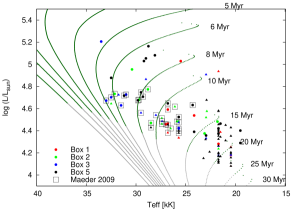
Some of the conclusions derived in this paper were already obtained by Hunter et al. (2008a), based on the same observational sample as the one scrutinized here, but only based on a subset of the stellar models presented in Paper I rather than on detailed population synthesis. Maeder et al. (2009) argued that the conclusions of Hunter et al. were unwarranted, due to the dispersion of the sample stars in mass, age, rotation, and binarity (we ignore the suggestion of a metallicity spread, which is known to be small in the LMC). In their own analysis, where they reduced the sample size by a factor of about 4 to consider only stars of similar mass, they still maintained the dispersion in age (see Fig. 12), rotation and binarity, and found their models of rotating single stars to explain the observations satisfactorily.
We find the picture emerging from the reduced sample analyzed by Maeder et al. (2009) and that from Hunter et al. (2008a) not very different. This is in fact not surprising, since the restriction in mass applied by Maeder et al. is not necessary. The mass range of stars in the full sample is already so small (9…25 ), that the expected nitrogen enrichment is very similar throughout the considered mass range (cf. Fig. 8, and also Fig. 1 of Maeder et al. (2009)). This is in fact confirmed by their analysis, which shows the bands of potentially rotationally mixed stars in Figs. 3 and 4 of Maeder et al. (2009) being exactly the same, implying that the mass dependence is negligible. While Maeder et al. conclude that the stars in Box 3 agree with single star models, we do the same, only we note that binary evolution provides an alternative explanation for these stars.
Maeder et al. also find stars in Box 2 in their reduced samples, with a similar proportion as they occur in the full sample. While Maeder et al. argue that they may occur due to binary effects and thus do not disturb the agreement of single star predictions with the observations, Meynet et al. (2011) argue that massive slowly rotating nitrogen-rich main sequence stars could be single stars undergoing magnetic braking, as proposed by Hunter et al. (2008a). Only the fraction of rapidly rotating stars without strong nitrogen enrichment (Box 1) in the Maeder et al. (2009) sample is smaller than in the full sample, which is due to the small size of the samples of Maeder et al. However, of course, all Box 1 stars in the full sample remain to be explained.
In any case, we developed the population synthesis approach as presented in this paper in order to construct a tool to analyze also diverse stellar samples in a statistically sound way. The spread in age, mass and rotation (and in principle, metallicity) is fully accounted for by our method. Our new results reinforce the uncomfortable conclusions of Hunter et al. (2008a) that two significant groups of massive core hydrogen burning stars stand out as being in conflict with evolutionary models, posing a challenge to the concept of rotational mixing.
6 Conclusions
Through detailed single star population synthesis modeling, we have tried to reproduce the properties of the largest homogeneous sample of early B-type stars in the LMC. This sample is the first for which nitrogen surface abundances have been determined for a wide range in projected rotational velocities. Uncertain mixing parameters in the underlying stellar evolution models (overshooting and rotational mixing) have been calibrated such that they reproduce the observed main-sequence widening deduced from the sharp drop in rotational velocities (Paper I, Vink et al. 2010), as well as the observed pattern of nitrogen enrichment as a function of the projected rotation velocity in the majority of fast rotators (Hunter et al. 2008a).
We confirm quantitatively the result of Hunter et al. (2008a) that two sub-populations of stars, namely rapidly rotating, unenriched stars and slowly rotating, nitrogen-rich stars (Boxes 1a and 2 in Fig. 10), are not reproduced by a population synthesis model for single stars.
While the group of rapidly rotating nitrogen-rich stars (Box 3) is, by construction, in qualitative agreement with our simulation, only about half of the number of predicted stars are found to be present in the observational sample. Although possibly explained by uncertainties in our method (see Sec. 4.1), predictions of close binary evolution models, which also produce nitrogen-rich rapid rotators, tend to increase this discrepancy.
We find it unlikely that the group of slowly rotating nitrogen-rich stars (Box 2 in Fig. 10) is produced via mass transfer and subsequent tidal spin-down in close binary systems, as a binary population which could produce these stars would likely overpopulate the group of rapidly rotating nitrogen-rich stars (see Sec. 5.1). At present, it appears plausible that some of the unexplained slowly rotating, nitrogen-rich stars are affected by magnetic fields (cf. the magnetic field measurements for Galactic stars with similar properties; Morel et al. 2008).
While a detailed physical prescription of possible magnetic effects in stellar models is currently not available, several binary effects are much better understood. Therefore, it appears promising to perform a binary population synthesis of massive main sequence stars in the near future, which will give quantitative constraints on the relative importance of binaries in the various subgroups. In fact, this appears to be required in order to arrive at solid conclusions on the nature of the group of rapidly rotation nitrogen-rich stars, and, thereby, obtain clear evidence for the universality of rotational mixing in massive stars.
Further light should be shed on this by the ongoing Tarantula Survey (Evans et al. 2010), which has targeted over 1000 stars in the 30 Doradus of the LMC. 30 Dor is the largest H ii region in the Local Group, containing a large number of very massive stars. The new survey is tailored for the detection of binarity, so will help sample the mass range above 30 , where mixing effects should be more significants, and therefore more easily detectable.
Acknowledgements.
We thank Georges Meynet, the referee of this paper, for many helpful comments and suggestions. SdM acknowledges support for this work provided by NASA through Hubble Fellowship grant HST-HF-51270.01-A awarded by the Space Telescope Science Institute, which is operated by the Association of Universities for Research in Astronomy, Inc., for NASA, under contract NAS 5-26555.References
- Aerts et al. (2009) Aerts, C., Puls, J., Godart, M., & Dupret, M. 2009, A&A, 508, 409
- Asplund et al. (2005) Asplund, M., Grevesse, N., & Sauval, A. J. 2005, in Astronomical Society of the Pacific Conference Series, Vol. 336, Cosmic Abundances as Records of Stellar Evolution and Nucleosynthesis, ed. T. G. Barnes, III & F. N. Bash, 25
- Babel & Montmerle (1997) Babel, J. & Montmerle, T. 1997, A&A, 323, 121
- Balona (1994) Balona, L. A. 1994, MNRAS, 268, 119
- Bosch et al. (2009) Bosch, G., Terlevich, E., & Terlevich, R. 2009, AJ, 137, 3437
- Bouret et al. (2003) Bouret, J., Lanz, T., Hillier, D. J., et al. 2003, ApJ, 595, 1182
- Brott et al. (2010) Brott, I., de Mink, S. E., Cantiello, M., et al. 2010, A&A, submitted
- Cantiello et al. (2009) Cantiello, M., Langer, N., Brott, I., et al. 2009, A&A, 499, 279
- Chabrier (2003) Chabrier, G. 2003, PASP, 115, 763
- Cranmer (2005) Cranmer, S. R. 2005, ApJ, 634, 585
- de Mink et al. (2009) de Mink, S. E., Cantiello, M., Langer, N., et al. 2009, A&A, 497, 243
- Dufton et al. (2005) Dufton, P. L., Ryans, R. S. I., Trundle, C., et al. 2005, A&A, 434, 1125
- Dufton et al. (2006) Dufton, P. L., Smartt, S. J., Lee, J. K., et al. 2006, A&A, 457, 265
- Endal & Sofia (1976) Endal, A. S. & Sofia, S. 1976, ApJ, 210, 184
- Evans et al. (2010) Evans, C. J., Bastian, N., Beletsky, Y., et al. 2010, in IAU Symposium, Vol. 266, IAU Symposium, 35–40
- Evans et al. (2006) Evans, C. J., Lennon, D. J., Smartt, S. J., & Trundle, C. 2006, A&A, 456, 623
- Evans et al. (2005) Evans, C. J., Smartt, S. J., Lee, J.-K., et al. 2005, A&A, 437, 467
- Gies & Lambert (1992) Gies, D. R. & Lambert, D. L. 1992, ApJ, 387, 673
- Grevesse et al. (1996) Grevesse, N., Noels, A., & Sauval, A. J. 1996, in Astronomical Society of the Pacific Conference Series, Vol. 99, Cosmic Abundances, ed. S. S. Holt & G. Sonneborn, 117
- Heger & Langer (2000) Heger, A. & Langer, N. 2000, ApJ, 544, 1016
- Heger et al. (2000) Heger, A., Langer, N., & Woosley, S. E. 2000, ApJ, 528, 368
- Herrero (1993) Herrero, A. 1993, Space Science Reviews, 66, 137
- Hubeny & Lanz (1995) Hubeny, I. & Lanz, T. 1995, ApJ, 439, 875
- Hunter et al. (2009a) Hunter, I., Brott, I., Langer, N., et al. 2009a, A&A, 496, 841
- Hunter et al. (2008a) Hunter, I., Brott, I., Lennon, D. J., et al. 2008a, ApJ, 676, L29
- Hunter et al. (2007) Hunter, I., Dufton, P. L., Smartt, S. J., et al. 2007, A&A, 466, 277
- Hunter et al. (2008b) Hunter, I., Lennon, D. J., Dufton, P. L., et al. 2008b, A&A, 479, 541
- Hunter et al. (2009b) Hunter, I., Lennon, D. J., Dufton, P. L., et al. 2009b, A&A, 504, 211
- Iglesias & Rogers (1996) Iglesias, C. A. & Rogers, F. J. 1996, ApJ, 464, 943
- Kaper et al. (1997) Kaper, L., Henrichs, H. F., Fullerton, A. W., et al. 1997, A&A, 327, 281
- Keller et al. (1999) Keller, S. C., Wood, P. R., & Bessell, M. S. 1999, A&AS, 134, 489
- Kroupa (2001) Kroupa, P. 2001, MNRAS, 322, 231
- Kurt & Dufour (1998) Kurt, C. M. & Dufour, R. J. 1998, in Revista Mexicana de Astronomia y Astrofisica, vol. 27, Vol. 7, Revista Mexicana de Astronomia y Astrofisica Conference Series, ed. R. J. Dufour & S. Torres-Peimbert, 202
- Langer (1991) Langer, N. 1991, A&A, 252, 669
- Langer et al. (2008) Langer, N., Cantiello, M., Yoon, S.-C., et al. 2008, in IAU Symposium, Vol. 250, IAU Symposium, ed. F. Bresolin, P. A. Crowther, & J. Puls, 167–178
- MacGregor & Cassinelli (2003) MacGregor, K. B. & Cassinelli, J. P. 2003, ApJ, 586, 480
- Maeder (1987) Maeder, A. 1987, A&A, 178, 159
- Maeder (2000) Maeder, A. 2000, New Astronomy Review, 44, 291
- Maeder et al. (2009) Maeder, A., Meynet, G., Ekström, S., & Georgy, C. 2009, Communications in Asteroseismology, 158, 72
- Martayan et al. (2008) Martayan, C., Diago, P., Gutiérrez-Soto, J., et al. 2008, ArXiv e-prints
- Martins et al. (2005) Martins, F., Schaerer, D., & Hillier, D. J. 2005, A&A, 436, 1049
- Martins et al. (2004) Martins, F., Schaerer, D., Hillier, D. J., & Heydari-Malayeri, M. 2004, A&A, 420, 1087
- Mason et al. (2009) Mason, B. D., Hartkopf, W. I., Gies, D. R., Henry, T. J., & Helsel, J. W. 2009, AJ, 137, 3358
- Meynet et al. (2011) Meynet, G., Eggenberger, P., & Maeder, A. 2011, A&A, 525, L11+
- Meynet & Maeder (2000) Meynet, G. & Maeder, A. 2000, A&A, 361, 101
- Mokiem et al. (2007) Mokiem, M. R., de Koter, A., Evans, C. J., et al. 2007, A&A, 465, 1003
- Mokiem et al. (2006) Mokiem, M. R., de Koter, A., Evans, C. J., et al. 2006, A&A, 456, 1131
- Morel et al. (2006) Morel, T., Butler, K., Aerts, C., Neiner, C., & Briquet, M. 2006, A&A, 457, 651
- Morel et al. (2008) Morel, T., Hubrig, S., & Briquet, M. 2008, A&A, 481, 453
- Packet (1981) Packet, W. 1981, A&A, 102, 17
- Papoulis (1984) Papoulis, A. 1984, Probability, Random Variables, and Stochastic Processes (New York: McGraw-Hil)
- Peimbert et al. (2007) Peimbert, M., Luridiana, V., & Peimbert, A. 2007, ApJ, 666, 636
- Petrovic et al. (2005) Petrovic, J., Langer, N., & van der Hucht, K. A. 2005, A&A, 435, 1013
- Porter & Rivinius (2003) Porter, J. M. & Rivinius, T. 2003, PASP, 115, 1153
- Prinja & Howarth (1988) Prinja, R. K. & Howarth, I. D. 1988, MNRAS, 233, 123
- Przybilla et al. (2010) Przybilla, N., Firnstein, M., Nieva, M. F., Meynet, G., & Maeder, A. 2010, A&A, 517, A38
- Puls et al. (2008) Puls, J., Vink, J. S., & Najarro, F. 2008, A&A Rev., 16, 209
- Salpeter (1955) Salpeter, E. E. 1955, ApJ, 121, 161
- Sana et al. (2009) Sana, H., Gosset, E., & Evans, C. J. 2009, MNRAS, 400, 1479
- Sana et al. (2008) Sana, H., Gosset, E., Nazé, Y., Rauw, G., & Linder, N. 2008, MNRAS, 386, 447
- Sana & Le Bouquin (2010) Sana, H. & Le Bouquin, J. 2010, in Revista Mexicana de Astronomia y Astrofisica Conference Series, Vol. 38, Revista Mexicana de Astronomia y Astrofisica Conference Series, 27–29
- Spruit (2002) Spruit, H. C. 2002, A&A, 381, 923
- Townsend et al. (2010) Townsend, R. H. D., Oksala, M. E., Cohen, D. H., Owocki, S. P., & ud-Doula, A. 2010, ApJ, 714, L318
- Townsend et al. (2004) Townsend, R. H. D., Owocki, S. P., & Howarth, I. D. 2004, MNRAS, 350, 189
- Trundle et al. (2007) Trundle, C., Dufton, P. L., Hunter, I., et al. 2007, A&A, 471, 625
- ud-Doula & Owocki (2002) ud-Doula, A. & Owocki, S. P. 2002, ApJ, 576, 413
- Vacca et al. (1996) Vacca, W. D., Garmany, C. D., & Shull, J. M. 1996, ApJ, 460, 914
- Vink et al. (2010) Vink, J. S., Brott, I., Gräfener, G., et al. 2010, A&A, 512, L7
- Vink et al. (2000) Vink, J. S., de Koter, A., & Lamers, H. J. G. L. M. 2000, A&A, 362, 295
- Vink et al. (2001) Vink, J. S., de Koter, A., & Lamers, H. J. G. L. M. 2001, A&A, 369, 574
- Vrancken et al. (2000) Vrancken, M., Lennon, D. J., Dufton, P. L., & Lambert, D. L. 2000, A&A, 358, 639
- Wade et al. (2006) Wade, G. A., Fullerton, A. W., Donati, J., et al. 2006, A&A, 451, 195
- Wolff (1968) Wolff, S. C. 1968, PASP, 80, 281
- Yoon & Langer (2005) Yoon, S. & Langer, N. 2005, A&A, 443, 643
- Yoon et al. (2006) Yoon, S.-C., Langer, N., & Norman, C. 2006, A&A, 460, 199
Appendix A The LMC Sample
In Fig. 13 we show the mass and projected rotational velocity distributions of our sample. In the upper panels, the targets are divided into the VLT-FLAMES fields. The rotational velocity distributions in both fields are very similar. The total mass distribution is dominated by N11 stars at high masses, while NGC 2004 contributes mainly to the lower-mass end.
We divided our sample into single and binary stars, as shown in the middle and lower panels of Fig. 13, respectively. The color coding corresponds to our selection effects that are later applied to each star of our population synthesis (see discussion in Sec. 3.3). The single star velocity distribution is well represented by those stars with measured nitrogen abundances (yellow panels). Around 50 is a peak of low gravity objects (orange), which is somewhat sensitive to our overshooting calibration. A value of 50 is also comparable to the expected the line broadening due to macro turbulence, therefore, these stars could be rotating at lower velocities.
The mass distribution of single stars with measured nitrogen abundances is also representative of the mass distribution of the total single star sample. Nitrogen abundances were not determined for the limited sample of the most massive stars owing to the problems of modeling the N iii line. The binary velocity distribution shows three peaks (at 30, 100 and 200 ), which may well be not statistically significant given the small number of stars.
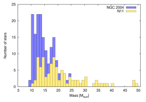 |
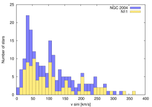 |
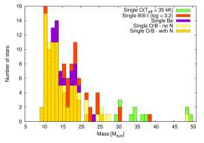 |
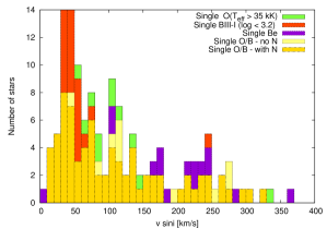 |
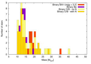 |
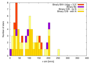 |