Volatility made observable at last

Abstract— The Cartier-Perrin theorem, which was published in 1995 and is expressed in the language of nonstandard analysis, permits, for the first time perhaps, a clear-cut mathematical definition of the volatility of a financial asset. It yields as a byproduct a new understanding of the means of returns, of the beta coefficient, and of the Sharpe and Treynor ratios. New estimation techniques from automatic control and signal processing, which were already successfully applied in quantitative finance, lead to several computer experiments with some quite convincing forecasts.

Keywords—Time series, quantitative finance, trends, returns, volatility, beta coefficient, Sharpe ratio, Treynor ratio, forecasts, estimation techniques, numerical differentiation, nonstandard analysis.

1 Introduction

Although volatility, which reflects the price fluctuations, is ubiquitous in quantitative finance (see, e.g., [3, 18, 22, 28, 32, 37], and the references therein), Paul Wilmott writes rightly ([37], chap. 49, p. 813):
Quite frankly, we do not know what volatility currently is, never mind what it may be in the future.
Our title is explained by sentences like the following one in Tsay’s book ([35], p. 98):
…volatility is not directly observable …
The lack moreover of any precise mathematical definition leads to multiple ways for computing volatility which are by no means equivalent and might even be sometimes misleading (see, e.g., [20]). Our theoretical formalism and the corresponding computer simulations will confirm what most practitioners already know. It is well expressed by Gunn ([21], p. 49):
Volatility is not only referring to something that fluctuates sharply up and down but is also referring to something that moves sharply in a sustained direction. The existence of trends [11] for time series, which should be viewed as the means, or averages, of those series, yields

• a natural and straightforward model-free definition of the variance (resp. covariance) of one (resp. two) time series,

• simple forecasting techniques which are based on similar techniques to those in [11, 12, 13, 14].

Exploiting the above approach to volatility for the return of some financial asset necessitates some care due to the highly fluctuating character of returns. This is accomplished by considering the means of the time series associated to the prices logarithms. The following results are derived as byproducts:

1. We complete [13] with a new definition of the classic beta coefficient for returns. It should bypass most of the existing criticisms.

2. The Sharpe ([30, 31]) and Treynor ratios, which are famous performance measures for trading strategies (see, e.g., [3, 28, 34, 37], and the references therein), are connected to a quite arbitrary financial time series. They might lead to new and useful trading indicators.

Remark 1

The graphical representation of all the above quantities boils down to the drawing of means which has been already successfully achieved in [11, 12, 13, 14].

Our paper is organized as follows. After recalling the Cartier-Perrin theorem [6], Section 2 defines (co)variances and volatility. In order to apply this setting to financial returns, Section 3 defines the means of returns and suggests definitions of the beta coefficient, and of the Sharpe and Treynor ratios. Numerous quite convincing computer experiments are shown in Section 4, which displays also excellent forecasts for the volatility. Some short discussions on the concept of volatility may be found in Section 5.

2 Mean, variance and covariance revisited

2.1 Time series via nonstandard analysis

2.1.1 Infinitesimal sampling

Take the time interval $[0,1]\subset\mathbb{R}$ and introduce as often in nonstandard analysis the infinitesimal sampling

$${\mathfrak{T}}=\{0=t_{0}<t_{1}<\dots<t_{\nu}=1\}$$

where $t_{i+1}-t_{i}$, $0\leq i<\nu$, is infinitesimal, i.e., “very small”. A time series $X(t)$ is a function $X:{\mathfrak{T}}\rightarrow\mathbb{R}$.

2.1.2 $S$-integrability

The Lebesgue measure on ${\mathfrak{T}}$ is the function $m$ defined on ${{\mathfrak{T}}}\backslash\{1\}$ by $m(t_{i})=t_{i+1}-t_{i}$. The measure of any interval $[c,d[\subset\mathfrak{I}$, $c\leq d$, is its length $d-c$. The integral over $[c,d[$ of the time series $X(t)$ is the sum

$$\int_{[c,d[}Xdm=\sum_{t\in[c,d[}X(t)m(t)$$

$X$ is said to be $S$-integrable if, and only if, for any interval $[c,d[$ the integral $\int_{[c,d[}|X|dm$ is limited and, if $d-c$ is infinitesimal, also infinitesimal.

2.1.3 Continuity and Lebesgue integrability

$X$ is $S$-continuous at $t_{\iota}\in{\mathfrak{T}}$ if, and only if, $f(t_{\iota})\simeq f(\tau)$ when $t_{\iota}\simeq\tau$. $X$ is said to be almost continuous if, and only if, it is $S$-continuous on ${\mathfrak{T}}\setminus R$, where $R$ is a rare subset. $X$ is Lebesgue integrable if, and only if, it is $S$-integrable and almost continuous.

2.1.4 Quick fluctuations

A time series ${\mathcal{X}}:{\mathfrak{T}}\rightarrow\mathbb{R}$ is said to be quickly fluctuating, or oscillating, if, and only if, it is $S$-integrable and $\int_{A}{\mathcal{X}}dm$ is infinitesimal for any quadrable subset.

2.1.5 The Cartier-Perrin theorem

Let $X:{\mathfrak{T}}\rightarrow\mathbb{R}$ be a $S$-integrable time series. Then, according to the Cartier-Perrin theorem [6], the additive decomposition

$$\boxed{X(t)=E(X)(t)+X_{\tiny{\rm fluctuation}}(t)}$$ (1)

holds where

• the mean, or average, $E(X)(t)$ is Lebesgue integrable,

• $X_{\tiny{\rm fluctuation}}(t)$ is quickly fluctuating.

The decomposition (1) is unique up to an infinitesimal.

Remark 2

$E(X)(t)$, which is “smoother” than $X(t)$, provides a mathematical justification [11] of the trends in technical analysis (see, e.g., [2, 25]).

Remark 3

Calculations of the means and of its derivatives, if they exist, are deduced, via new estimation techniques, from the denoising results in [17, 27] (see also [19]), which extend the familiar moving averages, which are classic in technical analysis (see, e.g., [2, 25]).

2.2 Variances and covariances

2.2.1 Squares and products

Take two $S$-integrable time series $X(t)$, $Y(t)$, such that their squares and the squares of $E(X)(t)$ and $E(Y)(t)$ are also $S$-integrable. The Cauchy-Schwarz inequality shows that the products

• $X(t)Y(t)$, $E(X)(t)E(Y)(t)$,

• $E(X)(t)Y_{\tiny{\rm fluctuation}}(t)$, $X_{\tiny{\rm fluctuation}}(t)E(Y)(t)$,

• $X_{\tiny{\rm fluctuation}}(t)Y_{\tiny{\rm fluctuation}}(t)$

are all $S$-integrable.

2.2.2 Differentiability

Assume moreover that $E(X)(t)$ and $E(Y)(t)$ are differentiable in the following sense: there exist two Lebesgue integrable time series $f,g:{\mathfrak{T}}\rightarrow\mathbb{R}$, such that, $\forall\leavevmode\nobreak\ t\in{\mathfrak{T}}$, with the possible exception of a limited number of values of $t$, $E(X)(t)=E(X)(0)+\int_{0}^{t}f(\tau)d\tau$, $E(Y)(t)=E(Y)(0)+\int_{0}^{t}g(\tau)d\tau$. Integrating by parts shows that the products $E(X)(t)Y_{\tiny{\rm fluctuation}}(t)$ and $X_{\tiny{\rm fluctuation}}(t)E(Y)(t)$ are quickly fluctuating [9].

Remark 4

Let us emphasize that the product

$$X_{\tiny{\rm fluctuation}}(t)Y_{\tiny{\rm fluctuation}}(t)$$

is not necessarily quickly fluctuating.

2.2.3 Definitions

1. The covariance of two time series $X(t)$ and $Y(t)$ is

   $$\mbox{\rm cov}(XY)(t) = E\left((X-E(X))(Y-E(Y))\right)(t)$$

   $$\simeq E(XY)(t)-E(X)(t)\times E(Y)(t)$$

2. The variance of the time series $X(t)$ is

   $$\mbox{\rm var}(X)(t) = E\left((X-E(X))^{2}\right)(t)$$

   $$\simeq E(X^{2})(t)-\left(E(X)(t)\right)^{2}$$

3. The volatility of $X(t)$ is the corresponding standard deviation

   $$\boxed{\mbox{\rm vol}(X)(t)=\sqrt{\mbox{\rm var}(X)(t)}}$$ (2)

The volatility of a quite arbitrary time series seems to be precisely defined here for the first time.

Remark 5

Another possible definition of the volatility (see [20]), which is not equivalent to Equation (2), is the following one

$$E\left(|X-E(X)|\right)(t)$$

It will not be exploited here.

3 Returns

3.1 Definition

Assume from now on that, for any $t\in{\mathfrak{T}}$,

$$0<m<X(t)<M$$

where $m$, $M$ are appreciable. This is a realistic assumption if $X(t)$ is the price of some financial asset $\mathfrak{A}$. The logarithmic return, or log-return, of $X$ with respect to some limited time interval $\Delta T>0$ is the time series $R_{\Delta T}$ defined by

$$R_{\Delta T}(X)(t)=\ln\left(\frac{X(t)}{X(t-\Delta T)}\right)=\ln X(t)-\ln X(t-\Delta T)$$

From $\frac{X(t)}{X(t-\Delta T)}=1+\frac{X(t)-X(t-\Delta T)}{X(t-\Delta T)}$, we know that

$$R_{\Delta T}(X)(t)\simeq\frac{X(t)-X(t-\Delta T)}{X(t-\Delta T)}$$ (3)

if $X(t)-X(t-\Delta T)$ is infinitesimal. The right handside of Equation (3) is the arithmetic return.

The normalized logarithmic return is

$$r_{\Delta T}(X)(t)=\frac{R_{\Delta T}(t)}{\Delta T}$$ (4)

3.2 Mean

3.2.1 Definition

Replace $X:{\mathfrak{T}}\rightarrow\mathbb{R}$ by

$$\ln X:{\mathfrak{T}}\rightarrow{\mathbb{R}},\quad t\mapsto\ln\left(X(t)\right)$$

where the logarithms of the prices are taken into account. Apply the Cartier-Perrin theorem to $\ln X$. The mean, or average, of $r_{\Delta T}(t)$ given by Equation (4) is

$$\boxed{\bar{r}_{\Delta T}(X)(t)=\frac{E(\ln X)(t)-E(\ln X)(t-\Delta T)}{\Delta T}}$$ (5)

As a matter of fact $r_{\Delta T}(X)$ and $\bar{r}_{\Delta T}(X)$ are related by

$$r_{\Delta T}(X)(t)=\bar{r}_{\Delta T}(X)(t)+\text{quick fluctuations}$$

Assume that $E(X)$ and $E(\ln X)$ are differentiable according to Section 2.2.2. Call the derivative of $E(\ln X)$ the normalized mean logarithmic instantaneous return and write

$$\boxed{\bar{r}(X)(t)=\frac{d}{dt}E(\ln X)(t)}$$ (6)

Note that $E(\ln X)(t)\simeq\ln\left(E(X)(t)\right)$ if in Equation (1) $X_{\tiny{\rm fluctuation}}(t)\simeq 0$. Then $\bar{r}(X)(t)\simeq\frac{\frac{d}{dt}E(X)(t)}{E(X)(t)}$.

3.2.2 Application to beta

Take two assets $\mathfrak{A}$ and $\mathfrak{B}$ such that their normalized logarithmic returns $r_{\Delta T}({\mathfrak{A}})(t)$ and $r_{\Delta T}({\mathfrak{B}})(t)$, defined by Equation (4), exist. Following Equation (5), consider the space curve $t,\bar{r}_{\Delta T}({\mathfrak{A}})(t),\bar{r}_{\Delta T}({\mathfrak{B}})(t)$ in the Euclidean space with coordinates $t,x,y$. Its projection on the $x,y$ plane is the plane curve $\mathfrak{C}$ defined by

$$x_{\mathfrak{C}}(t)=\bar{r}_{\Delta T}({\mathfrak{A}})(t),y_{\mathfrak{C}}(t)=\bar{r}_{\Delta T}({\mathfrak{B}})(t)$$

The tangent of $\mathfrak{C}$ at a regular point, which is defined by $\frac{dx_{\mathfrak{C}}(t)}{dt},\frac{dy_{\mathfrak{C}}(t)}{dt}$, yields, if $\frac{dx_{\mathfrak{C}}(t)}{dt}\neq 0$,

$$\Delta y_{\mathfrak{C}}\approx\beta(t)\Delta x_{\mathfrak{C}}$$ (7)

where

• $\Delta x_{\mathfrak{C}}=x_{\mathfrak{C}}(t+h)-x_{\mathfrak{C}}(t)$, $\Delta y_{\mathfrak{C}}=y_{\mathfrak{C}}(t+h)-y_{\mathfrak{C}}(t)$;

• $h\in\mathbb{R}$ is “small”;

• $${\beta(t)=\frac{\frac{dy_{\mathfrak{C}}(t)}{dt}}{\frac{dx_{\mathfrak{C}}(t)}{dt}}}$$ (8)

When $y_{\mathfrak{C}}(t)$ may be viewed locally as a smooth function of $x_{\mathfrak{C}}(t)$, Equation (8) becomes

$${\beta(t)=\frac{dy_{\mathfrak{C}}}{dx_{\mathfrak{C}}}}$$

3.2.3 The Treynor ratio of an asset

Let $\beta_{\mathfrak{M}}({\mathfrak{A}})(t)$ be the beta coefficient defined in Section 3.2.2 for ${\mathfrak{A}}$ with respect to the market portfolio $\mathfrak{M}$. Define the Treynor ratio and the instantaneous Treynor ratio of $\mathfrak{A}$ with respect to $\mathfrak{M}$ respectively by

$$\boxed{\text{TR}_{{\mathfrak{M}},\Delta T}({\mathfrak{A}})(t)=\frac{\bar{r}_{\Delta T}({\mathfrak{A}})(t)}{\beta_{\mathfrak{M}}({\mathfrak{A}})(t)},\quad\text{TR}_{{\mathfrak{M}}}({\mathfrak{A}})(t)=\frac{\bar{r}({\mathfrak{A}})(t)}{\beta_{\mathfrak{M}}({\mathfrak{A}})(t)}}$$

3.3 Volatility

Formulae (2), (4), (5), (6) yield the following mathematical definition of the volatility of the asset $\mathfrak{A}$:

$$\boxed{{\text{\bf vol}}_{\Delta T}({\mathfrak{A}})(t)=\sqrt{E(r_{\Delta T}-\bar{r}_{\Delta T})^{2}(t)}}$$ (9)

which yields

$$\boxed{{\text{\bf vol}}_{\Delta T}({\mathfrak{A}})(t)\simeq\sqrt{E(r_{\Delta T}^{2})(t)-(\bar{r}_{\Delta T}(t))^{2}}}$$

The value at time $t$ of ${\text{\bf vol}}_{\Delta T}({\mathfrak{A}})$ may be viewed as the actual volatility (see, e.g., [37], chap. 49, pp. 813-814).

Remark 6

A crucial difference between Formula (9) and the usual historical, or realized, volatilities (see, e.g., [37], chap. 49, pp. 813-814) lies in the presence of a non-constant mean. It is often assumed to be $0$ in the existing literature.

Remark 7

There is no connection with

• the implied volatility, which is connected to the Black-Scholes modeling (see, e.g., [37], chap. 49, pp. 813-814),

• the recent model-free implied volatility (see [4], and [23, 29]), although the origin of our viewpoint may be partly traced back to our model-free control strategy ([10, 24]).

3.4 The Sharpe ratio of an asset

Define the Sharpe ratio of the asset ${\mathfrak{A}}$ by

$$\boxed{\text{SR}_{\Delta T}({\mathfrak{A}})(t)=\frac{\bar{r}_{\Delta T}({\mathfrak{A}})(t)}{{\text{\bf vol}}_{\Delta T}({\mathfrak{A}})(t)}}$$ (10)

According to [1], p. 52, it is quite close to some utilization of the Sharpe ratio in high-frequency trading.

4 Computer experiments

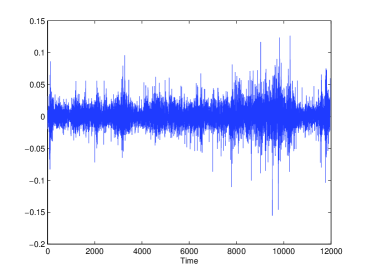
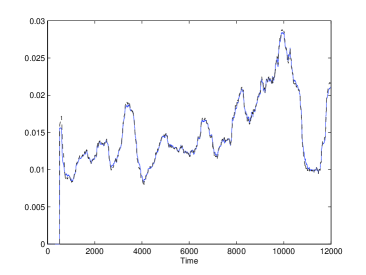
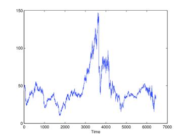
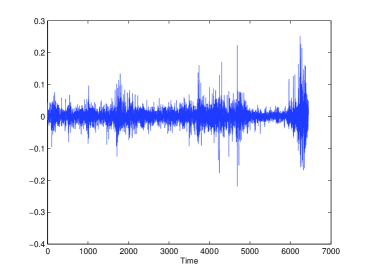
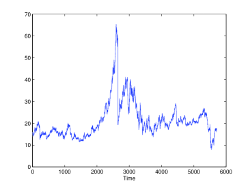
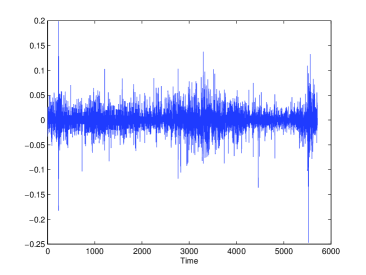
We have utilized the following three listed shares:

1. IBM from 1962-01-02 to 2009-07-21 (11776 days) (Figures 1 and 2),

2. JPMORGAN CHASE (JPM) from 1983-12-30 until 2009-07-21 (6267 days) (Figures 3),

3. COCA COLA (CCE) from 1986-11-24 until 2009-07-21 (5519 days) (Figures 4).

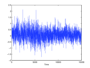
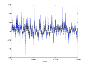
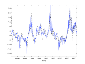
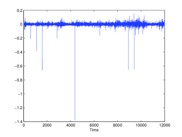
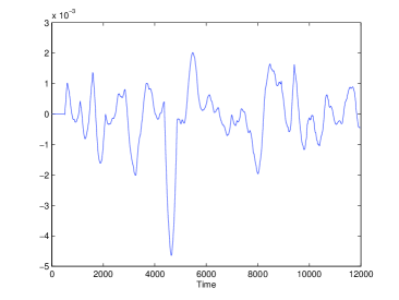
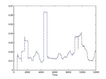
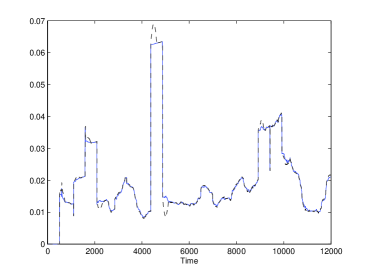
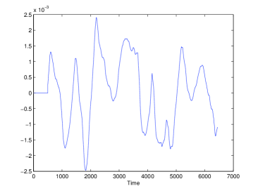
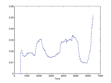
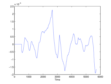
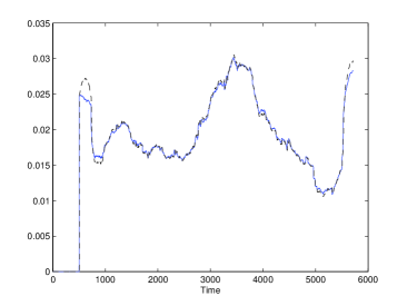
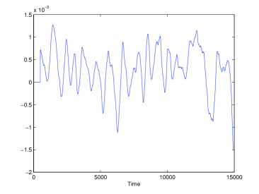
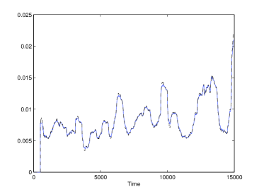
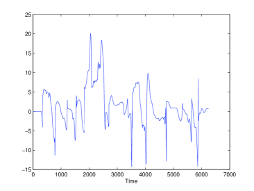
Figures 1 and 3 show a “better” behavior for the normalized mean logarithmic return (6), i.e., $\bar{r}(t)$ is less affected by an abrupt short price variation. Such variations are nevertheless causing important variations on our volatility, with only a “slow mean return”. We suggest an adaptive threshold for attenuating this annoying feature, which does not reflect well the price behavior. Note the excellent volatility forecasts which are obtained via elementary numerical recipes as in [11, 12, 13, 14]. Our forecasting results, which are easily computable, seem to be more reliable than those obtained via the celebrated ARCH type techniques, which go back to Engle (see [36] and the references therein).

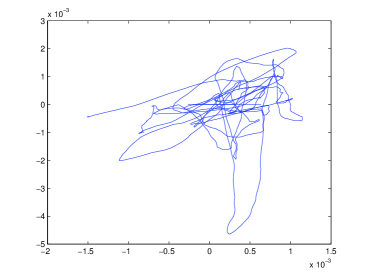
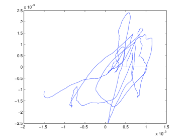
The beta coefficients is computed with respect to the S&P 500 (see Figures 5). The results displayed in Figures 4 are obtained via the numerical techniques of [13].

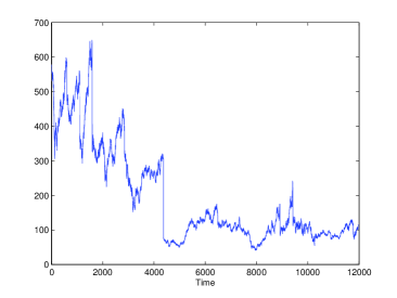
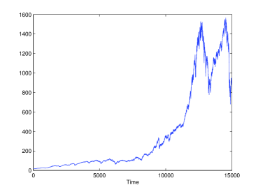
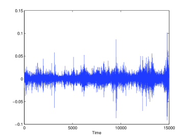
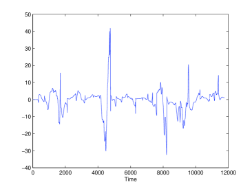
Figure 7 displays the Sharpe ratio of S&P 500. With $\Delta t=10$ a trend is difficult to guess in Figure 7-(a). Figure 7-(b) on the other hand, where $\Delta t=100$, exhibits a well-defined trend which yields a quite accurate forecasting of 10 days.

(a) Daily price

(b) Normalized logarithmic return $r(t)$

(c) Normalized mean logarithmic return $\bar{r}(t)$

(d) $\text{\bf vol}({IBM})(t)$ (–) and 5 days forecasting (- -)

(e) $\text{\bf vol}({IBM})(t)$ (–) and 20 days forecasting (- -)

Figure 1: IBM

(a) Modified normalized logarithmic return $r(t)$

(b) $\text{\bf vol}({IBM})(t)$ (–) and 20 days forecasting (- -)

Figure 2: IBM

(a) Daily price

(b) Modified normalized logarithmic return $r(t)$

(c) Normalized mean logarithmic return $\bar{r}(t)$

(d) $\text{\bf vol}({JPM})(t)$ (–) and 20 days forecasting (- -)

Figure 3: JPMORGAN CHASE (JPM)

(a) Daily price

(b) Modified normalized logarithmic return $r(t)$

(c) Normalized mean logarithmic return $\bar{r}(t)$

(d) $\text{\bf vol}({CCE})(t)$ (–) and 20 days forecasting (- -)

Figure 4: COCA COLA (CCE)

(a) Daily price

(b) Modified normalized logarithmic return $r(t)$

(c) Normalized mean logarithmic return $\bar{r}(t)$

(d) $\text{\bf vol}({S\&P500})(t)$ (–) and 20 days forecasting (- -)

Figure 5: S&P 500

(a) $\mathfrak{C}$: $\bar{r}_{IBM}(\bar{r}_{S\&P500}$)

(b) IBM’s $\beta(t)$

(c) $\mathfrak{C}$: $\bar{r}_{JPM}(\bar{r}_{S\&P500})$

(d) JPM’s $\beta(t)$

Figure 6:

(a) $\text{SR}_{10}({S\&P500})$

(b) $\text{SR}_{100}({S\&P500})$ (–) and 10 days forecasting (- -)

(c) Zoom of 7-(b)

Figure 7:

5 Conclusion

Although we have proposed a precise and elegant mathematical definition of volatility, which

• yields efficient and easily implementable computations,

• will soon be exploited for a dynamic portfolio management [15],

the harsh criticisms against its importance in financial engineering should certainly not be dismissed (see, e.g., [33]). Note for instance that we have not tried here to forecast extreme events, i.e., abrupt changes (see [16]) with this tool. This aim has been already quite successfully achieved in [11, 12, 13, 14], not via volatility but by taking advantage of indicators that are related to prices and not to returns.

References

- [1] Alridge I., High-Frequency Trading. Wiley, 2010.
- [2] Béchu T., Bertrand E., Nebenzahl J., L’analyse technique ( éd.). Economica, 2008.
- [3] Bodie Z., Kane A., Marcus A.J., Investments (7th ed.). McGraw-Hill, 2008.
- [4] Britten-Jones M., Neuberger A., Option prices, implied price processes, and stochastic volatility. J. Finance, vol. 55, pp. 839-866, 2000.
- [5] Campbell J.Y., Lo A.W., MacKinlay A.C., The Econometrics of Financial Markets. Princeton University Press, 1997.
- [6] Cartier P., Perrin Y., Integration over finite sets. In Nonstandard Analysis in Practice, F. & M. Diener (Eds), Springer, 1995, pp. 195-204.
- [7] Diener F., Diener M., Tutorial. In F. & M. Diener (Eds): Nonstandard Analysis in Practice. Springer, pp. 1-21, 1995.
- [8] Diener F., Reeb G., Analyse non standard. Hermann, 1989.
- [9] Fliess M., Analyse non standard du bruit. C.R. Acad. Sci. Paris Ser. I, vol. 342, pp. 797-802, 2006.
- [10] Fliess M., Join C., Commande sans modèle et commande à modèle restreint. e-STA, vol. 5 (n∘ 4), pp. 1-23, 2008 (available at http://hal.archives-ouvertes.fr/inria-00288107/en/).
- [11] Fliess M., Join C., A mathematical proof of the existence of trends in financial time series. In Systems Theory Modeling, Analysis and Control, A. El Jai, L. Afifi, E. Zerrik (Eds), Presses Universitaires de Perpignan, 2009, pp. 43–62 (available at http://hal.archives-ouvertes.fr/inria-00352834/en/).
-
[12]
Fliess M., Join C., Towards new technical indicators for trading
systems and risk management. IFAC Symp. System Identif.,
Saint-Malo, 2009 (available at
http://hal.archives-ouvertes.fr/inria-00370168/en/). - [13] Fliess M., Join C., Systematic risk analysis first steps towards a new definition of beta. COGIS, Paris, 2009 (available at http://hal.archives-ouvertes.fr/inria-00425077/en/).
[14]
Fliess M., Join C., Delta hedging in financial
engineering: towards a model-free setting. 18th Medit. Conf.
Control Automat., Marrakech, 2010 (available at
http://hal.archives-ouvertes.fr/inria-00479824/en/). - [15] Fliess M., Join C., Hatt. F., A-t-on vraiment besoin de modèles probabilistes en ingénierie financière ?. Conf. médit. ingénierie sûre systèmes complexes, Agadir, 2011 (soon available at http://hal.archives-ouvertes.fr/).
- [16] Fliess M., Join C., Mboup M., Algebraic change-point detection. Applicable Algebra Engin. Communic. Comput., vol. 21, pp. 131-143, 2010.
[17]
Fliess M., Join C., Sira-Ramírez H.,
Non-linear estimation is easy. Int. J. Model. Identif.
Control, vol. 4, pp. 12-27, 2008 (available at
http//hal.archives-ouvertes.fr/inria-00158855/en/). - [18] Franke J., Härdle W.K., Hafner C.M., Statistics of Financial Markets (2nd ed.). Springer, 2008.
[19]
García Collado F.A., d’Andréa-Novel B., Fliess M.,
Mounier H., Analyse fréquentielle des dérivateurs algébriques.
XXIIe Coll. GRETSI, Dijon, 2009 (available at
http://hal.archives-ouvertes.fr/inria-00394972/en/). - [20] Goldstein D.G., Taleb N.N., We don’t quite know what we are talking about when we talk about volatility. J. Portfolio Management, vol. 33, pp. 84-86, 2007.
- [21] Gunn M., Trading Regime Analysis. Wiley, 2009.
- [22] Hull J.C., Options, Futures, and Other Derivatives (7th ed.). Prentice Hall, 2007.
- [23] Jiang G.J., Tian Y.S., The model-free implied volatility and its information content. Rev. Financial Studies, vol. 18, pp. 1305-1342, 2005.
[24]
Join C., Robert G., Fliess M., Vers une commande
sans modèle pour aménagements hydroélectriques en cascade. 6e
Conf. Internat. Francoph. Automat., Nancy, 2010 (available at
http//hal.archives-ouvertes.fr/inria-00460912/en/). - [25] Kirkpatrick C.D., Dahlquist J.R., Technical Analysis: The Complete Resource for Financial Market Technicians (2nd ed.). FT Press, 2010.
- [26] Lobry C., Sari T., Nonstandard analysis and representation of reality. Int. J. Control, vol. 81, pp. 517-534, 2008.
- [27] Mboup M., Join C., Fliess M., Numerical differentiation with annihilators in noisy environment. Numer. Algor., vol. 50, pp. 439-467, 2009.
- [28] Roncalli T., La gestion d’actifs quantitative. Economica, 2010.
- [29] Rouah F.D., Vainberg G., Option Pricing Models and Volatility. Wiley, 2007.
- [30] Sharpe W.F., Mutual fund performance. J. Business, vol. 39, pp. 119-138, 1966.
- [31] Sharpe W.F., The Sharpe ratio. J. Portfolio Management, vol. 21, pp. 49-58, 1994.
- [32] Sinclair E., Volatility Trading. Wiley, 2008.
- [33] Taleb N.N., Errors, robustness, and the fourth quadrant. Int. J. Forecasting, vol. 25, pp. 744-759, 2009.
- [34] Treynor J.L., Treynor on Institutional Investing. Wiley, 2008.
- [35] Tsay R.S., Analysis of Financial Time Series (2nd ed.). Wiley, 2005.
- [36] Watson M., Bollerslev T., Russel J. (Eds), Volatility and Time Series Econometrics – Essays in Honor of Robert Engle. Oxford University Press, 2010.
- [37] Wilmott P., Paul Wilmott on Quantitative Finance, 3 vol. (2nd ed.). Wiley, 2006.