Persistent Robotic Tasks:
Monitoring and Sweeping in Changing Environments

Abstract

We present controllers that enable mobile robots to persistently monitor or sweep a changing environment. The changing environment is modeled as a field which grows in locations that are not within range of a robot, and decreases in locations that are within range of a robot. We assume that the robots travel on given closed paths. The speed of each robot along its path is controlled to prevent the field from growing unbounded at any location. We consider the space of speed controllers that can be parametrized by a finite set of basis functions. For a single robot, we develop a linear program that is guaranteed to compute a speed controller in this space to keep the field bounded, if such a controller exists. Another linear program is then derived whose solution is the speed controller that minimizes the maximum field value over the environment. We extend our linear program formulation to develop a multi-robot controller that keeps the field bounded. The multi-robot controller has the unique feature that it does not require communication among the robots. Simulation studies demonstrate the robustness of the controllers to modeling errors, and to stochasticity in the environment.

I Introduction

In this paper we treat the problem of controlling robots to perpetually act in a changing environment, for example to clean an environment where material is constantly collecting, or to monitor an environment where uncertainty is continually growing. Each robot has only a small footprint over which to act (e.g. to sweep or to sense). The difficulty is in controlling the robots to move so that their footprints visit all points in the environment regularly, spending more time in those locations where the environment changes quickly, without neglecting the locations where it changes more slowly. This scenario is distinct from most other sweeping and monitoring scenarios in the literature because the task cannot be “completed.” That is to say, the robots must continually move to satisfy the objective. We consider the situation in which robots are constrained to move on fixed paths, along which we must control their speed. We consider both the single robot and multi-robot cases. Figure 1 shows three robots monitoring an environment using controllers designed with our method.

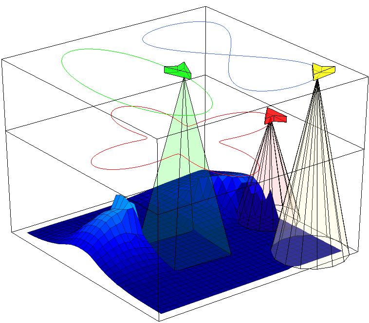
Figure 1: A persistent monitoring task using three robots with heterogeneous, limited range sensors. The surface shows the accumulation function, indicating the quantity of material to be removed in a cleaning application, or the uncertainty at each point in a sensing application. The accumulation function grows when a robot’s footprint is not over it, and decreases when the footprint is over it. Each robot controls its speed along its prescribed path so as to keep the surface as low as possible everywhere.

We model the changing environment with a scalar valued function defined, which we call the accumulation function. The function behaves analogously to dust accumulating over a floor. When a robot’s footprint is not over a point in the environment, the accumulation function grows at that point at a constant rate, as if the point were collecting dust. When a robot’s footprint is over the point, the accumulation function decreases at a constant rate, as if the dust were being vacuumed by the robot. The rates of growth and decrease can be different at different points in the environment.

This model is applicable to situations in which the task of the robot is to remove material that is collecting in the environment, for example cleaning up oil in the ocean around a leaking well [1], vacuuming dirt from the floor of a building [2], or tending to produce in an agricultural field [3]. It is also applicable to monitoring scenarios in which the state of the environment changes at each point, and we want to maintain up-to-date knowledge of this changing state. Some examples include monitoring temperature, salinity, or chlorophyll in the ocean [4], maintaining estimates of coral reef health [5], or monitoring traffic congestion over a city [6]. These applications all share the property that they can never be completed, because the environment is always changing. If the robot were to stop moving, the oil would collect beyond acceptable levels, or the knowledge of the ocean temperature would become unacceptably outdated. For this reason we call these applications persistent tasks. In this paper, we assume that the model is known either from the physics of the environment, from a human expert, or from an initial survey of the environment. However we show analytically and in simulation that our controllers are robust to model errors.

We focus on the situation in which the robots are given fixed, closed paths on which to travel, and we have to carry out the persistent task only by regulating their speed. This is relevant in many real-world scenarios. For example, in the case that the robots are autonomous cars, they may be constrained to move on a particular circuit of roads in a city to avoid traffic congestion, or in the case of autonomous aircraft, they may be constrained to fly along a particular path to stay away from commercial air traffic, or to avoid being detected by an adversary. Even in the case of vacuuming the floor of a building, the robots may be required to stay along a prescribed path so as not to interfere with foot traffic. Furthermore, if we have the freedom to plan the robot’s path, we can employ an off-line planner to generate paths that are optimal according to some metric (using the planner in [7] for example), then apply the procedure in this paper to control the speed along the path. Decoupling the path planning from the speed control in this way is a well-established technique for dealing with complex trajectory planning problems [8].

I-A Contributions

Our approach to the problem is to represent the space of all possible speed controllers with a finite set of basis functions, where each possible speed controller is a linear combination of those basis functions. A rich class of controllers can be represented in this way. Using this representation as our foundation, the main contributions of this paper are the following.

1. We formally introduce the idea of persistent tasks for robots in changing environments, and propose a tractable model for designing robot controllers.

2. Considering the space of speed controllers parametrized by a finite set of basis functions, we formulate a linear program (LP) whose solution is a speed controller which guarantees that the accumulation function eventually falls below, and remains below, a known bound everywhere. If the LP is infeasible, then no controller in the space that will keep the accumulation function bounded.

3. We formulate an LP whose solution is the optimal speed controller—that which eventually minimizes the maximum of the accumulation function over all locations.

4. We generalize to the multi-robot case. We find an LP whose solution is a controller which guarantees that the accumulation function falls below, and stays below, a known bound. The multi-robot controller does not require communication between robots.

We do not find the optimal controller for the multi-robot case, however, as it appears that this controller cannot be found as the solution to an LP. We demonstrate the performance of the controllers in numerical simulations, and show that they are robust to stochastic and deterministic errors in the environment model, and to unmodeled robot vehicle dynamics.

It is desirable to cast our speed control problem as an LP since LPs can be solved efficiently with off-the-shelf solvers [9]. This is enabled by our basis function representation. The use of basis functions is a common, and powerful method for function approximation [10], and is frequently used in areas such as compressive sampling [11], adaptive control [12], and machine learning [13]. Our LP formulations also incorporate both maximum and minimum limits on the robot’s speed, which can be different at different points on the path. This is important because we may want a robot not to exceed a certain speed around a sharp turn, for example, while it can go much faster on a long straightaway.

I-B Related Work

Our work is related to the large body of existing research on environmental monitoring, sensor sweep coverage, lawn mowing and milling, and patrolling. In the environmental monitoring literature (also called objective analysis in meteorological research [14] and Kriging in geological research [15]), authors often use a probabilistic model of the environment, and estimate the state of that model using a Kalman-like filter. Then robots are controlled so as to maximize a metric on the quality of the state estimate. For example, the work in [16] controls robots to move in the direction of the gradient of mutual information. More recently, the authors of [17] and [18] control vehicles to decrease the variance of their estimate of the state of the environment. This is accomplished in a distributed way by using average consensus estimators to propagate information among the robots. Similarly, [19] proposes a gradient based controller to decrease the variance of the estimate error in a time changing environment. In [20] sensing robots are coordinated to move in a formation along level curves of the environmental field. In [21] the authors find optimal trajectories over a finite horizon if the environmental model satisfies a certain spatial separation property. Also, in [22] the authors solve a dynamic program (DP) over a finite horizon to find the trajectory of a robot to minimize the variance of the estimate of the environment, and a similar DP approach was employed in [23] over short time horizons. Many other works exist in this vein.

Although these works are well-motivated by the uncontested successes of Kalman filtering and Kriging in real-world estimation applications, they suffer from the fact that planning optimal trajectories under these models requires the solution of an intractable dynamic program, even for a static environment. One must resort to myopic methods, such as gradient descent (as in [16, 17, 18, 20, 19]), or solve the DP approximately over a finite time horizon (as in [21, 22, 23]). Although these methods have great appeal from an estimation point of view, little can be proved about the comparative performance of the control strategies employed in these works. The approach we take in this paper circumvents the question of estimation by formulating a new model of growing uncertainty in the environment. Under this model, we can solve the speed planning problem over infinite time, while maintaining guaranteed levels of uncertainty in a time-changing environment. Thus we have used a less sophisticated environment model in order to obtain stronger results on the control strategy. Because our model is based on the analogy of dust collecting in an environment, we also solve infinite horizon sweeping problems with the same method.

Our problem in this paper is also related to sweep coverage, or lawn mowing and milling problems, in which robots with finite sensor footprints move over an environment so that every point in the environment is visited at least once by a robot. Lawn mowing and milling has been treated in [24] and other works. Sweep coverage has recently been studied in [25], and in [26] efficient sweep coverage algorithms are proposed for ant robots. A survey of sweep coverage is given in [27]. Our problem is significantly different from these because our environment is dynamic, thereby requiring continual re-milling or re-sweeping. A different notion of persistent surveillance has been considered in [28] and [29], where a persistent task is defined as one whose completion takes much longer than the life of a robot. While the terminology is similar, our problem is more concerned with the task (sweeping or monitoring) itself than with power requirements of individual robots.

A problem more closely related to ours is that of patrolling [30, 31], where an environment must be continually surveyed by a group of robots such that each point is visited with equal frequency. Similarly, in [32] vehicles must repeatedly visit the cells of a gridded environment. Also, continual perimeter patrolling is addressed in [33]. In another related work, a region is persistently covered in [34] by controlling robots to move at constant speed along predefined paths. Our work is different from these, however, in that we treat the situation in which different parts of the environment may require different levels of attention. This is a significant difference as it induces a difficult resource trade-off problem as one typically finds in queuing theory [35], or dynamic vehicle routing [36, 37]. In [38], the authors consider unequal frequency of visits in a gridded environment, but they control the robots using a greedy method that does not have performance guarantees.

Indeed, our problem can be seen as a dynamic vehicle routing problem with some unique features. Most importantly, we control the speed of the robots along a pre-planned path, whereas the typical dynamic vehicle routing problem considers planning a path for vehicles that move at constant speed. Also, in our case all the points under a robot’s footprint are serviced simultaneously, whereas typically robots service one point at a time in dynamic vehicle routing. Finally, in our case servicing a point takes an amount of time proportional to the size of the accumulation function at that point, whereas the service time of points in dynamic vehicle routing is typically independent of that points wait-time.

The paper is organized as follows. In Section II we set up the problem and define some basic notions. In Section III two LPs are formulated, one of which gives a stabilizing controller, and the other one an optimal controller. Multiple robots are addressed in Section IV. The performance and robustness of the controllers are illustrated in simulations in Section V. Finally, Section VI gives conclusions and extensions.

II Problem Formulation and Stability Notions

In this section we formalize persistent tasks, introduce the notion of a field stabilizing controller, and provide a necessary and sufficient conditions for field stability.

II-A Persistent Tasks

Consider a compact environment $\mathcal{E}\subset{\mathbb{R}}^{2}$, and a finite set of points of interest $Q\subseteq\mathcal{E}$. The environment contains a closed curve $\gamma:[0,1]\to{\mathbb{R}}^{2}$, where $\gamma(0)=\gamma(1)$. (See Figure 2 for an illustration.) The curve is parametrized by $\theta\in[0,1]$, and we assume without loss of generality that $\theta$ is the arc-length parametrization. The environment also contains a single robot (we will generalize to multiple robots in Section IV) whose motion is constrained along the path $\gamma$. The robot’s position at a time $t$ can be described by $\theta(t)$, its position along the curve $\gamma$. The robot is equipped with a sensor with finite footprint $\mathcal{B}(\theta)\subset\mathcal{E}$ (For example, the footprint could be a disk of radius $r$ centered at the robot’s position). Our objective is to control the speed $v$ of the robot along the curve. We assume that for each point $\theta$ on the curve, the maximum possible robot speed is $v_{\max}(\theta)$ and the minimum robot speed is $v_{\min}(\theta)>0$. This allows us to express constraints on the robot speed at different points on the curve. For example, for safety considerations, the robot may be required to move more slowly in certain areas of the environment, or on high curved sections of the path. To summarize, the robot is described by the triple $\mathcal{R}:=(\mathcal{B},v_{\min},v_{\max})$.

A time-varying field $Z:Q\times{\mathbb{R}}_{\geq 0}\to{\mathbb{R}}_{\geq 0}$, which we call the accumulation function, is defined on the points of interest $Q$. This field may describe a physical quantity, such as the amount of oil on the surface of a body of water. Alternatively, the field may describe the robot’s uncertainty about the state of each point of interest. We assume that at each point $\mathbf{q}\in Q$, the field $Z$ increases (or is produced) at a constant rate $p(\mathbf{q})$. When the robot footprint is covering $\mathbf{q}$, it consumes $Z$ at a constant rate $c(\mathbf{q})$, so that when a point $\mathbf{q}$ is covered, the net rate of decrease is $p(\mathbf{q})-c(\mathbf{q})$. Thus, $Z$ evolves according to the following differential equation (with initial conditions $Z(\mathbf{q},0)$ and $\theta(0)$):

$$\dot{Z}(\mathbf{q},t)=\begin{cases}p(\mathbf{q}),&\text{if $\mathbf{q}\notin\mathcal{B}\big{(}\theta(t)\big{)}$},\\ p(\mathbf{q})-c(\mathbf{q}),&\text{if $\mathbf{q}\in\mathcal{B}\big{(}\theta(t)\big{)}$ and $Z(\mathbf{q},t)>0$},\\ 0,&\text{if $\mathbf{q}\in\mathcal{B}\big{(}\theta(t)\big{)}$ and $Z(\mathbf{q},t)=0$},\end{cases}$$ (1)

where for each $\mathbf{q}\in Q$, we have $c(\mathbf{q})>p(\mathbf{q})>0$. In this paper, we assume that we know the model parameters $p(\mathbf{q})$ and $c(\mathbf{q})$. It is reasonable to assume knowledge of $c(\mathbf{q})$ since it pertains to the performance of the robot. For example, in an oil cleanup application, the consumption rate of oil of the robot can be measured in a laboratory environment or in field trials prior to control design. As for the production rate, $p(\mathbf{q})$, this must be estimated from the physics of the environment, from a human expert (e.g. an oil mining engineer in the case of an oil well leak), or it can be measured in a preliminary survey of the environment. However, the accuracy of the model is not crucial, as we show analytically and in simulations that our method has strong robustness with respect to errors in $p(\mathbf{q})$. The production function can also be estimated and incorporated into the controller on-line, though we save the development of an on-line strategy for future work.

With this notation, we can now formally define a persistent task.

Definition II.1 (Persistent Tasks).

A persistent task is a tuple $(\mathcal{R},\gamma,Q,p,c)$, where $\mathcal{R}$ is the robot model, $\gamma$ is the curve followed by the robot, $Q$ is the set of points of interest, and $p$ and $c$ are the production and consumption rates of the field, respectively.

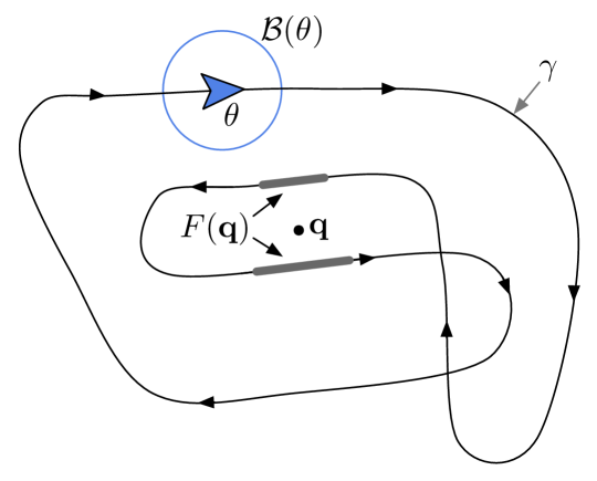
Figure 2: An illustration of a curve $\gamma$ followed by the robot. The robot is located at $\theta$ and has footprint $\mathcal{B}(\theta)$. The set $F(\mathbf{q})$ of robot positions $\theta$ for which the footprint covers $q$ are shown as thick grey segments of the curve.

In general, for a given persistent task, the commanded speed $v$ could depend on the current position $\theta$, the field $Z$, the initial conditions $\theta(0)$ and $Z(\mathbf{q},0)$, and time $t$. Thus, defining the set of initial conditions as $\mathrm{IC}:=(\theta(0),Z(\mathbf{q},0))$, a general controller has the form $v(\theta,Z,\mathrm{IC},t)$. For the reader’s convenience, the notation used in this paper is summarized in Table I.

II-B Field Stability and Feasibility

In this section we formalize the problem of stabilizing the field in a persistent task. As a first consideration, a suitable controller should keep the field bounded everywhere, independent of the initial conditions. This motivates the following definition of stability.

Definition II.2 (Field Stabilizing Controller).

A speed controller field stabilizes a persistent task if the field is always eventually bounded, independent of initial conditions. That is, if there exists a $Z_{\max}<+\infty$ such that for every $\mathbf{q}\in Q$ and initial condition $Z(\mathbf{q},0)$ and $\theta(0)$, we have

$$\limsup_{t\to+\infty}Z(\mathbf{q},t)\leq Z_{\max}.$$

Note that in this definition of stability, for every initial condition, the field eventually enters the interval $[0,Z_{\max}]$.

There are some persistent tasks for which no controller is field stabilizing. This motivates the notion of feasibility.

Definition II.3 (Feasible Persistent Task).

A persistent task is feasible if there exists a field stabilizing speed controller.

As stated above, for a given persistent task, a general speed controller can be written as $v(\theta,Z,\mathrm{IC},t)$. However, in the remainder of the paper we will focus on a small subset of speed controllers which we call periodic position-feedback controllers. In these controllers, the speed only depends on the robot’s current position $\theta\in[0,1]$. The controllers are periodic in the sense that the speed at a point $\theta$ is the same on each cycle of the path. The controller can be written as

$$v:[0,1]\to{\mathbb{R}}_{>0},$$

where each $\theta\in[0,1]$ is mapped to a speed $v(\theta)$ satisfying the bounds $v_{\min}(\theta)\leq v(\theta)\leq v_{\max}(\theta)$. These controllers have the advantage that they do not require information on the current state of the field $Z$, only its model parameters $p(\mathbf{q})$ and $c(\mathbf{q})$. While it may seem restrictive to limit our controllers to this special form, the following result shows that it is not.

Proposition II.4 (Periodic Position-Feedback Controllers).

If a persistent task can be stabilized by a general controller $v(\theta,Z,\mathrm{IC},t)$, then it can be stabilized by a periodic position-feedback controller $v(\theta)$.

The proof of Proposition II.4 is given in Appendix VI-A, and relies on the statement and proof of the upcoming result in Lemma II.5. Therefore, we encourage the reader to postpone reading the proof until after Lemma II.5.

We will now investigate conditions for a controller to be field stabilizing and for a persistent task to be feasible. Let us define a function which maps each point $\mathbf{q}\in Q$, to the curve positions $\theta$ for which $\mathbf{q}$ is covered by the robot footprint. To this end, we define

$$F(\mathbf{q}):=\{\theta\in[0,1]\;|\;\mathbf{q}\in\mathcal{B}(\theta)\}.$$

An illustration of the curve, the robot footprint, and the set $F(\mathbf{q})$ is shown in Figure 2. (In Section V we discuss how this set can be computed in practice.)

Given a controller $\theta\mapsto v(\theta)$, we define two quantities: 1) the cycle time, or period, $T$, and 2) the coverage time per cycle $\tau(\mathbf{q})$. Since $v(\theta)>0$ for all $\theta$, the robot completes one full cycle of the closed curve in time

$$T:=\int_{0}^{1}\frac{1}{v(\theta)}d\theta.$$ (2)

During each cycle, the robot’s footprint is covering the point $\mathbf{q}$ only when $\theta(t)\in F(\mathbf{q})$. Thus the point $\mathbf{q}$ is covered for

$$\tau(\mathbf{q}):=\int_{F(\mathbf{q})}\frac{1}{v(\theta)}d\theta,$$ (3)

time units during each complete cycle.

With these definitions we can give a necessary and sufficient condition for a controller to stabilize a persistent task. In Section III, we develop a method for testing if this condition can be satisfied by a speed controller.

Lemma II.5 (Stability condition).

Given a persistent task, a controller $v(\theta)$ is field stabilizing if and only if

$$c(\mathbf{q})\int_{F(\mathbf{q})}\frac{1}{v(\theta)}d\theta>p(\mathbf{q})\int_{0}^{1}\frac{1}{v(\theta)}d\theta$$ (4)

for every $\mathbf{q}\in Q$. Applying the definitions in (2) and (3), the condition can be expressed as $\tau(\mathbf{q})>\big{(}p(\mathbf{q})/c(\mathbf{q})\big{)}T$.

The lemma has a simple intuition. For stability, the field consumption per cycle must exceed the field production per cycle, for each point $\mathbf{q}\in Q$. We now prove the result.

Proof.

Consider a point $\mathbf{q}\in Q$, and the set of curve positions $F(\mathbf{q})$ for which $\mathbf{q}$ is covered by the robot footprint. Given the speed controller $v$, we can compute the cycle time $T$ in (2). Then, let us consider the change in the field from $Z(\mathbf{q},t)$ to $Z(\mathbf{q},t+T)$, where $t\geq 0$.

Define an indicator function $\mathbf{I}:[0,1]\times Q\to\{0,1\}$ as $\mathbf{I}(\theta,\mathbf{q})=1$ for $\theta\in F(\mathbf{q})$ and $0$ otherwise. Then, from (1) we have that

$$\dot{Z}(\mathbf{q},t)\geq p(\mathbf{q})-c(\mathbf{q})\mathbf{I}(\theta(t),\mathbf{q}),$$

for all values of $Z(\mathbf{q},t)$, with equality if $Z(\mathbf{q},t)>0$. Integrating the above expression over $[t,t+T]$ we see that

$$Z(\mathbf{q},t+T)-Z(\mathbf{q},t) \geq p(\mathbf{q})T-c(\mathbf{q})\int_{t}^{t+T}\mathbf{I}(\theta(\tau),\mathbf{q})d\tau$$

$$=p(\mathbf{q})T-c(\mathbf{q})\tau(\mathbf{q}),$$ (5)

where $\tau(\mathbf{q})$ is defined in (3), and the equality follows from the fact that $\mathbf{I}(\theta(t),\mathbf{q})$ is simply an indicator function on whether or not the footprint is covering $\mathbf{q}$ at a given time. From (5) we see that for the field to be eventually bounded by some $Z_{\max}$ for all initial conditions $Z(\mathbf{q},0)$, we require that $\tau(\mathbf{q})>p(\mathbf{q})/c(\mathbf{q})T$ for all $\mathbf{q}\in Q$.

To see that the condition is also sufficient, suppose that $\tau(\mathbf{q})>p(\mathbf{q})/c(\mathbf{q})T$. Then there exists $\epsilon>0$ such that $p(\mathbf{q})T-c(\mathbf{q})\tau(\mathbf{q})=-\epsilon$. If $Z(\mathbf{q},t)>\big{(}c(\mathbf{q})-p(\mathbf{q})\big{)}T$, then the field at the point $\mathbf{q}\in Q$ is strictly positive over the entire interval $[t,t+T]$, implying that

$$Z(\mathbf{q},t+T)=Z(\mathbf{q},t)-\epsilon.$$

Thus, from every initial condition, $Z(\mathbf{q},t)$ moves below $\big{(}c(\mathbf{q})-p(\mathbf{q})\big{)}T$. Additionally, note that for each $\bar{t}$ in the interval $[t,t+T]$, we trivially have that $Z(\mathbf{q},\bar{t})\leq Z(\mathbf{q},t)+p(\mathbf{q})T$. Thus, we have that there exists a finite time $\bar{t}$ such that for all $t\geq\bar{t}$,

$$Z(\mathbf{q},t)\leq\big{(}c(\mathbf{q})-p(\mathbf{q})\big{)}T+p(\mathbf{q})T=c(\mathbf{q})T.$$

Since $Q$ is finite, there exists a single $\epsilon>0$ such that for every point $\mathbf{q}\in Q$ we have $\tau(\mathbf{q})-p(\mathbf{q})/c(\mathbf{q})T>\epsilon$. Hence, letting $Z_{\max}=\max_{\mathbf{q}\in Q}c(\mathbf{q})T$, we see that $Z$ is stable for all $\mathbf{q}$, completing the proof. ∎

In the following sections we will address two problems, determining a field stabilizing controller, and determining a minimizing controller, defined as follows:

Problem II.6 (Persistent Task Metrics).

Given a persistent task, determine a periodic position-feedback controller $v:[0,1]\to{\mathbb{R}}_{>0}$ that satisfies the speed constraints (i.e., $v(\theta)\in\big{[}v_{\min}(\theta),v_{\max}(\theta)\big{]}$ for all $\theta\in[0,1]$), and

1. is field stabilizing; or

2. minimizes the maximum steady-state field $\mathcal{H}(v)$:

   $$\mathcal{H}(v):=\max_{\mathbf{q}\in Q}\left(\limsup_{t\to+\infty}Z(\mathbf{q},t)\right).$$

In Section III we will show that by writing the speed controller in terms of a set of basis functions, problems (i) and (ii) can be solved using linear programs. In Section IV we will solve problem (i) for multiple robots.

III Single Robot Speed Controllers:
Stability and Optimality

In this paper we focus on a finite set of points of interest $Q=\{\mathbf{q}_{1},\ldots,\mathbf{q}_{m}\}$. These $m$ locations could be specific regions of interest, or they could be a discrete approximation of the continuous space obtained by, for example, laying a grid down on the environment. In the Section V we will show examples of both scenarios. Our two main results are given in Theorems III.1 and III.8, which show that a field stabilizing controller, and a controller minimizing $\mathcal{H}(v)$, can each be found by solving an appropriate linear program.

To begin, it will be more convenient to consider the reciprocal speed controller $v^{-1}(\theta):=1/v(\theta)$, with its corresponding constraints

$$\frac{1}{v_{\max}(\theta)}\leq v^{-1}(\theta)\leq\frac{1}{v_{\min}(\theta)}.$$

Now, our approach is to consider a finite set of basis functions $\{\beta_{1}(\theta),\ldots,\beta_{n}(\theta)\}$. Example basis functions include (a finite subset of) the Fourier basis or Gaussian basis [10]. In what follows we will use rectangular functions as the basis:

$$\beta_{j}(\theta)=\begin{cases}1,&\text{if $\theta\in[(j-1)/n,j/n)$}\\ 0,&\text{otherwise},\end{cases}$$ (6)

for each $j\in\{1,\ldots,n\}$. This basis, which provides a piecewise constant approximation to a curve, has the advantage that we will easily be able to incorporate the speed constraints $v_{\min}(\theta)$ and $v_{\max}(\theta)$ into the controller.

Then let us consider reciprocal speed controllers of the form

$$v^{-1}(\theta)=\sum_{j=1}^{n}\alpha_{j}\beta_{j}(\theta),$$ (7)

where $\alpha_{1},\ldots,\alpha_{n}\in{\mathbb{R}}$ are free parameters that we will use to optimize the speed controller. A rich class of functions can be represented as a finite linear combination of basis functions, though not all functions can be represented this way. Limiting our speed controller to a linear parametrization allows us to find an optimal controller within that class, while preserving enough generality to give complex solutions that would be difficult to find in an ad hoc manner. In the following subsection we will consider the problem of synthesizing a field stabilizing controller.

III-A Synthesis of a Field Stabilizing Controller

In this section we will show that a field stabilizing speed controller of the form (7) can be found through the solution of a linear program. This result is summarized in Theorem III.1. We remind the reader that A summary of the mathematical symbols and their definitions is shown in Table I.

TABLE I: Table of Symbols

Symbol	Definition
$\mathcal{E}$	the environment.
$Q$	a set of points of interest in the environment $\mathcal{E}$.
$\mathbf{q}$	a point of interest in $Q$.
$\gamma$	a curve followed by the robot, and parametrized by $\theta$.
$v(\theta)$	the speed of the robot along the curve $\gamma$.
$\mathcal{R}$	the robot model, consisting of minimum and maximum speeds $v_{\min}(\theta)$ and $v_{\max}(\theta)$, and a robot footprint $\mathcal{B}(\theta)$.
$\mathcal{B}(\theta)$	The set of points in the environment covered by the robot’s footprint when positioned at $\theta$.
$F(\mathbf{q})$	the values of $\theta\in[0,1]$ along the curve $\gamma$ for which the point $\mathbf{q}$ is covered by the footprint.
$Z(\mathbf{q},t)$	the field (or accumulation function) at point $\mathbf{q}\in Q$ at time $t$.
$p(\mathbf{q})$	the rate of production of the field $Z$ at point $\mathbf{q}$.
$c(\mathbf{q})$	the rate of consumption of the field $Z$ when $\mathbf{q}$ is covered by the robot footprint.
$\beta(\theta)$	a basis function.
$\alpha$	a basis function coefficient, or parameter.
$T$	the time to complete one full cycle of the curve.
$\tau(\mathbf{q})$	the amount of time the point $\mathbf{q}\in Q$ is covered per cycle.
$\mathcal{H}(v)$	cost function (10) giving the steady-state maximum value of $Z(\mathbf{q},t)$

To begin, let us consider reciprocal speed controllers in the form of (7). Then for $\mathbf{q}_{i}\in Q$, the stability condition in Lemma II.5 becomes

$$\sum_{j=1}^{n}\alpha_{j}\int_{F(\mathbf{q}_{i})}\beta_{j}(\theta)d\theta>\frac{p(\mathbf{q}_{i})}{c(\mathbf{q}_{i})}\sum_{j=1}^{n}\alpha_{j}\int_{0}^{1}\beta_{j}(\theta)d\theta$$

Rearranging, we get

$$\sum_{j=1}^{n}\alpha_{j}K(\mathbf{q}_{i},\beta_{j})>0,$$

where we have defined

$$K(\mathbf{q}_{i},\beta_{j}):=\int_{F(\mathbf{q}_{i})}\beta_{j}(\theta)d\theta-\frac{p(\mathbf{q}_{i})}{c(\mathbf{q}_{i})}\int_{0}^{1}\beta_{j}(\theta)d\theta.$$ (8)

Finally, to satisfy the speed constraints we have that

$$\frac{1}{v_{\max}(\theta)}\leq\sum_{j=1}^{n}\alpha_{j}\beta_{j}(\theta)\leq\frac{1}{v_{\min}(\theta)}$$ (9)

For the rectangular basis in (6), the speed constraints become

$$\frac{1}{v_{\max}(j)}\leq\alpha_{j}\leq\frac{1}{v_{\min}(j)},$$

where

$$v_{\max}(j) =\inf_{\theta\in[(j-1)/n,j/n)}v_{\max}(\theta),\;\text{and}$$

$$v_{\min}(j) =\sup_{\theta\in[(j-1)/n,j/n)}v_{\min}(\theta).$$

Thus, we obtain the following result.

Theorem III.1 (Existence of a Field Stabilizing Controller).

A persistent task is stabilizable by a speed controller of the form (7) if and only if the following linear program is feasible:

minimize $$0$$

subject to $$\sum_{j=1}^{n}\alpha_{j}K(\mathbf{q}_{i},\beta_{j})>0 \forall\;i\in\{1,\ldots,m\}$$

$$\frac{1}{v_{\max}(j)}\leq\alpha_{j}\leq\frac{1}{v_{\min}(j)}, \forall\;j\in\{1,\ldots,n\},$$

where $K(\mathbf{q}_{i},\beta_{j})$ is defined in (8), and $\alpha_{1},\ldots,\alpha_{n}$ are the optimization variables.

Hence, we can solve for a field stabilizing controller using a simple linear program. The program has $n$ variables (one for each basis function coefficient), and $2n+m$ constraints (two for each basis function coefficient, and one for each point of interest in $Q$). One can easily solve linear programs with thousands of variables and constraints [9]. Thus, the problem of computing a field stabilizing controller can be solved for finely discretized environments with thousands of basis functions. Note that in the above lemma, we are only checking feasibility, and thus the cost function in the optimization is arbitrary. For simplicity we write the cost as $0$.

In Theorem III.1 the cost is set to $0$ to highlight the feasibility constraints. However, in practice, an important consideration is robustness of the controller to uncertainty and error in the model of the field evolution, and in the motion of the robot. Robustness of this type can be achieved by slightly altering the above optimization to maximize the stability margin. This is outlined in the following result.

Corollary III.2 (Robustness via Maximum Stability Margin).

The optimization

maximize $$B$$

$$\sum_{j=1}^{n}\alpha_{j}K(\mathbf{q}_{i},\beta_{j})\geq B \forall\;i\in\{1,\ldots,m\}$$

$$\frac{1}{v_{\max}(j)}\leq\alpha_{j}\leq\frac{1}{v_{\min}(j)}, \forall\;j\in\{1,\ldots,n\},$$

where $\alpha_{1},\ldots,\alpha_{n}$ and $B$ are the optimization variables, yields a speed controller which maximizes the stability margin, $\min_{\mathbf{q}_{i}\in Q}\sum_{j=1}^{n}\alpha_{j}K(\mathbf{q}_{i},\beta_{j})$. The controller

1. has the largest decrease in $Z(\mathbf{q}_{i},t)$ per cycle, and thus achieves steady-state in the minimum number of cycles.

2. is robust to errors in estimating the field production rate. If the robot’s estimate of the production rate at a field point $\mathbf{q}_{i}\in Q$ is $\bar{p}(\mathbf{q}_{i})$, and the true value is $p(\mathbf{q}_{i})\leq\bar{p}(\mathbf{q}_{i})+\epsilon$, then the field is stable provided that for each $\mathbf{q}_{i}\in Q$

   $$\epsilon<B\cdot c(\mathbf{q}_{i})\left(\sum_{j=1}^{n}\alpha_{j}\int_{0}^{1}\beta_{j}(\theta)d\theta\right)^{-1}.$$

Proof.

The first property follows directly from the fact that $\sum_{j=1}^{n}\alpha_{j}K(\mathbf{q}_{i},\beta_{j})$ is the amount of decrease of the field at point $\mathbf{q}_{i}$ in one cycle.

To see the second property, suppose that the optimization is based on a production rate $\bar{p}(\mathbf{q}_{i})$ for each $\mathbf{q}_{i}\in Q$, but the true production rate is given by $p(\mathbf{q}_{i}):=\bar{p}(\mathbf{q}_{i})+\epsilon$, where $\epsilon>0$. In solving the optimization above, we obtain a controller with a stability margin of $B>0$. For the true system to be stable we require that for each $\mathbf{q}_{i}\in Q$,

$$\sum_{j=1}^{n}\alpha_{j}\int_{F(\mathbf{q}_{i})}\beta_{j}(\theta)d\theta>\frac{\bar{p}(\mathbf{q}_{i})+\epsilon}{c(\mathbf{q}_{i})}\sum_{j=1}^{n}\alpha_{j}\int_{0}^{1}\beta_{j}(\theta)d\theta.$$

This can be rewritten as

$$\sum_{j=1}^{n}\alpha_{j}K(\mathbf{q}_{i},\beta_{j})>\frac{\epsilon}{c(\mathbf{q}_{i})}\sum_{j=1}^{n}\alpha_{j}\int_{0}^{1}\beta_{j}(\theta)d\theta,$$

from which we see that the true field is stable provided that $\epsilon<Bc(\mathbf{q}_{i})/\big{(}\sum_{j=1}^{n}\alpha_{j}\int_{0}^{1}\beta_{j}(\theta)d\theta\big{)}$ for each $\mathbf{q}_{i}\in Q$. ∎

Remark III.3 (Alternative Basis Functions).

Given an arbitrary set of basis functions, the inequalities in (9) yield an infinite (and uncountable) number of constraints, one for each $\theta\in[0,1]$. This means that for some basis functions the linear program in Theorem III.1 can not be solved exactly. However, in practice, an effective method is to simply enforce the constraints in (9) for a finite number of $\theta$ values, $\theta_{1},\ldots,\theta_{w}$. Each $\theta_{i}$ generates two constraints in the optimization. Then, we can tighten each constraint by $\xi>0$, yielding $1/v_{\max}(\theta_{i})+\xi\leq\sum_{j}\alpha_{j}\beta_{j}(\theta_{i})\leq 1/v_{\min}(\theta_{i})-\xi$ for each $i\in\{1,\ldots,w\}$. Choosing the number of $\theta$ values $w$ as large as possible given the available computational resources, we can then increase $\xi$ until the controller satisfies the original speed constraints. $\square$

III-B Synthesis of an Optimal Controller

In this section we look at Problem II.6 (ii), which is to minimize the maximum value attained by the field over the finite region of interest $Q$. That is, for a given persistent task, our goal is to minimize the following cost function,

$$\mathcal{H}(v)=\max_{\mathbf{q}\in Q}\left(\limsup_{t\to+\infty}Z(\mathbf{q},t)\right)$$ (10)

over all possible speed controllers $v$. At times we will refer to the maximum steady-state value for a point $\mathbf{q}$ using a speed controller $v$ as

$$\mathcal{H}(\mathbf{q},v):=\limsup_{t\to+\infty}Z(\mathbf{q},t)$$

Our main result of this section, Theorem III.8, is that $\mathcal{H}(v)$ can be minimized through a linear program. However, we must first establish intermediate results. First we show that if $v$ is a field stabilizing controller, then for every initial condition there exists a finite time $t^{*}$ such that $Z(\mathbf{q},t)\leq\mathcal{H}(v)$ for all $t\geq t^{*}$.

Proposition III.4 (Steady-State Field).

Consider a feasible persistent task and a field stabilizing speed controller. Then, there is a steady-state field

$$\bar{Z}:Q\times[0,1]\to{\mathbb{R}}_{\geq 0},$$

satisfying the following statements for each $\mathbf{q}\in Q$:

1. for every set of initial conditions $\theta(0)$ and $Z(\mathbf{q},0)$, there exists a time $t^{*}\geq 0$ such that

   $$Z(\mathbf{q},t)=\bar{Z}\big{(}\mathbf{q},\theta(t)\big{)},$$

   for all $t\geq t^{*}$.

2. there exists at least one $\theta\in[0,1]$ such that $\bar{Z}(\mathbf{q},\theta)=0$.

From the above result we see that from every initial condition, the field converges in finite time to a steady-state $\bar{Z}(\mathbf{q},\theta)$. In steady-state, the field $Z(\mathbf{q},t)$ at time $t$ depends only on $\theta(t)$ (and is independent of $Z(\mathbf{q},0)$). Each time the robot is located at $\theta$, the field is given by $\bar{Z}(\mathbf{q},\theta)$. Moreover, the result tells us that in steady-state there is always a robot position at which the field is reduced to zero. In order to prove Proposition III.4 we begin with the following lemma. Recall that the cycle-time for a speed controller $v$ is $T:=\int_{0}^{1}1/v(\theta)d\theta$.

Lemma III.5 (Field Reduced to Zero).

Consider a feasible persistent task and a field stabilizing speed controller. For every $\mathbf{q}\in Q$ and every set of initial conditions $Z(\mathbf{q},0)$ and $\theta(0)$, there exists a time $t^{*}>T$ such that

$$Z(\mathbf{q},t^{*}+aT)=0,$$ (11)

for all non-negative integers $a$.

Proof.

Consider any $\mathbf{q}\in Q$, and initial conditions $Z(\mathbf{q},0)$ and $\theta(0)$, and suppose by way of contradiction that the speed controller is stable but $Z(\mathbf{q},t)>0$ for all $t>T$. From Lemma II.5, if the persistent task is stable, then $c(\mathbf{q})\tau(\mathbf{q})>p(\mathbf{q})T$ for all $\mathbf{q}$. Thus, there exists $\epsilon>0$ such that $c(\mathbf{q})\tau(\mathbf{q})-p(\mathbf{q})T>\epsilon$ for all $\mathbf{q}\in Q$. From the proof of Lemma II.5, we have that

$$Z(\mathbf{q},t+T)-Z(\mathbf{q},t)=p(\mathbf{q})T-c(\mathbf{q})\tau(\mathbf{q})=-\epsilon.$$

Therefore, given $Z(\mathbf{q},0)$, we have that $Z(\mathbf{q},t^{*})=0$ for some finite $t^{*}>T$, a contradiction.

Next we will verify that if $Z(\mathbf{q},t^{*})=0$ for some $t^{*}>T$, then $Z(\mathbf{q},t^{*}+T)=0$. To see this, note that the differential equation (1) is piecewise constant. Given a speed controller $v(\theta)$, the differential equation is time-invariant, and admits unique solutions.

Based on this, consider two initial conditions for (1),

$$Z_{1}(\mathbf{q},0):=Z(\mathbf{q},t^{*}-T)\geq 0,\quad\theta_{1}(0):=\theta(t^{*}-T)=\theta(t^{*}),$$

and

$$Z_{2}(\mathbf{q},0):=Z(\mathbf{q},t^{*})=0,\quad\theta_{2}(0):=\theta(t^{*}).$$

Since (1) is time-invariant, we have that $Z_{1}(\mathbf{q},T)=Z(\mathbf{q},t^{*})=0$, and $Z_{2}(\mathbf{q},T)=Z(\mathbf{q},t^{*}+T)$. In addition, by uniqueness of solutions, we also know that $Z_{1}(\mathbf{q},0)\geq Z_{2}(\mathbf{q},0)$ implies that $Z_{1}(\mathbf{q},T)\geq Z_{2}(\mathbf{q},T)$. Thus, we have that $Z(\mathbf{q},t^{*})=0\geq Z(\mathbf{q},t^{*}+T)$, proving the desired result. ∎

The previous lemma shows that from every initial condition there exists a finite time $t^{*}$, after which the field at a point $\mathbf{q}$ is reduced to zero in each cycle. With this lemma we can prove Proposition III.4.

Proof of Proposition III.4.

In Lemma III.5 we have shown that for every set of initial conditions $Z(\mathbf{q},0)$, $\theta(0)$, there exists at time $t^{*}>T$ such that $Z(\mathbf{q},t^{*}+aT)=0$ for all non-negative integers $a$. Since $T$ is the cycle-time for the robot, we also know that $\theta(t^{*}+aT)=\theta(t^{*})$ for all $a$. Since (1) yields unique solutions, (11) uniquely defines $Z(\mathbf{q},t)$ for all $t\geq t^{*}$, with

$$Z(\mathbf{q},t+T)=Z(\mathbf{q},t)\quad\text{for all $t\geq t^{*}$.}$$

Hence, we can define the steady-state profile $\bar{Z}(\mathbf{q},\theta)$ as

$$\bar{Z}\big{(}\mathbf{q},\theta(t)\big{)}:=Z(\mathbf{q},t)\quad\text{for all $t\in[t^{*},t^{*}+T)$}.$$

Finally, we need to verify that $\bar{Z}(\mathbf{q},\theta)$ is independent of initial conditions. To proceed, suppose by way of contradiction that there are two sets of initial conditions $\theta_{1}(0)$, $Z_{1}(\mathbf{q},0)$, and $\theta_{2}(0)$, $Z_{2}(\mathbf{q},0)$ which yield different steady-state fields $\bar{Z}_{1}(\mathbf{q},\theta)$ and $\bar{Z}_{2}(\mathbf{q},\theta)$. That is, there exists $\tilde{\theta}$ such that $\bar{Z}_{1}(\mathbf{q},\tilde{\theta})\neq\bar{Z}_{2}(\mathbf{q},\tilde{\theta})$. Without loss of generality, assume that $\bar{Z}_{1}(\mathbf{q},\tilde{\theta})>\bar{Z}_{2}(\mathbf{q},\tilde{\theta})$. To obtain a contradiction, we begin by showing that this implies $\bar{Z}_{1}(\mathbf{q},\theta)\geq\bar{Z}_{2}(\mathbf{q},\theta)$ for all $\theta$. Note that $Z_{1}$ and $Z_{2}$ reach their steady-state profiles $\bar{Z}_{1}$ and $\bar{Z}_{2}$ in finite time. Thus, there exist times $t_{1},t_{2}\geq 0$ for which $\theta_{1}(t_{1})=\theta_{2}(t_{2})=\tilde{\theta}$, and $Z_{1}(\mathbf{q},t_{1})=\bar{Z}_{1}(\mathbf{q},\tilde{\theta})$, and $Z_{2}(\mathbf{q},t_{2})=\bar{Z}_{2}(\mathbf{q},\tilde{\theta})$. Since $Z_{1}(\mathbf{q},t_{1})>Z_{2}(\mathbf{q},t_{2})$, and since $Z$ is a continuous function of time, either i) $Z_{1}(\mathbf{q},t_{1}+t)>Z_{2}(\mathbf{q},t_{2}+t)$ for all $t\geq 0$, or ii) there exists a time $\bar{t}>0$ for which $Z_{1}(\mathbf{q},t_{1}+\bar{t})=Z_{2}(\mathbf{q},t_{2}+\bar{t})$, which by uniqueness of solutions implies $Z_{1}(\mathbf{q},t_{1}+t)=Z_{2}(\mathbf{q},t_{2}+t)$ for all $t\geq\bar{t}$. Thus, $Z_{1}(\mathbf{q},t_{1}+t)\geq Z_{2}(\mathbf{q},t_{2}+t)$ for all $t\geq 0$, implying that $\bar{Z}_{1}(\mathbf{q},\theta)\geq\bar{Z}_{2}(\mathbf{q},\theta)$ for all $\theta$.

From Lemma III.5, there exists a $\bar{\theta}$ for which $\bar{Z}_{1}(\mathbf{q},\bar{\theta})=0$. Since, $\bar{Z}_{1}(\mathbf{q},\theta)\geq\bar{Z}_{2}(\mathbf{q},\theta)$ for all $\theta$, we must have that $\bar{Z}_{2}(\mathbf{q},\bar{\theta})=0$. However, the value of $Z_{1}$ and $Z_{2}$ at $\bar{\theta}$ uniquely defines $\bar{Z}_{1}$ and $\bar{Z}_{2}$ for all $\theta$, implying that $\bar{Z}_{1}(\mathbf{q},\theta)=\bar{Z}_{2}(\mathbf{q},\theta)$, a contradiction. ∎

From Proposition III.4 we have shown the existence of a steady-state field $\bar{Z}(\mathbf{q},\theta)$ that is independent of initial conditions $Z(\mathbf{q},0)$ and $\theta(0)$.

Now, consider a point $\mathbf{q}\in Q$ and a field stabilizing speed controller $v(\theta)$, and let us solve for its steady-state field $\bar{Z}(\mathbf{q},\theta)$. To begin, let us write $F(\mathbf{q})$ (the set of $\theta$ values for which the point $\mathbf{q}$ is covered by the footprint) as a union of disjoint intervals

$$F(\mathbf{q})=[x_{1},y_{1}]\cup[x_{2},y_{2}]\cup\cdots\cup[x_{\ell},y_{\ell}],$$ (12)

where $\ell$ is a positive integer, and $y_{k}>x_{k}>y_{k-1}$ for each $k\in\{1,\ldots,\ell\}$. Thus, on the intervals $[x_{k},y_{k}]$ the point $\mathbf{q}$ is covered by the robot footprint, and on the intervals $[y_{k},x_{k+1}]$, the point $\mathbf{q}$ in uncovered. As an example, in Figure 2, the set $F(\mathbf{q})$ consists of two intervals, and thus $\ell=2$. An example of a speed controller and an example of a set $F(\mathbf{q})$ are shown in Figures 3a and 3b.

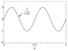
(a) A sample reciprocal speed controller $v(\theta)$

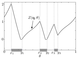
(b) The steady-state field $\bar{Z}(\mathbf{q},\theta)$. The set $F(\mathbf{q})$ consists of three intervals which are shaded on the $\theta$-axis. The steady-state profile is increasing outside of $F(\mathbf{q})$ and decreasing inside $F(\mathbf{q})$.

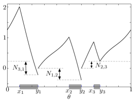
(c) The calculation of quantities $N_{1,2}$, $N_{2,3}$ and $N_{3,1}$. The values represent the maximum reduction from $y_{k-1}$ to $y_{k}$. Thus, $N_{1,2},N_{3,1}<0$ while $N_{2,3}>0$.

Figure 3: The steady-state field for a point $\mathbf{q}\in Q$. The set of $\theta$ values for which $\mathbf{q}$ is covered is given by $F(\mathbf{q})=[x_{1},y_{1}]\cup[x_{2},y_{2}]\cup[x_{3},y_{3}]$. The field is produced at a rate $p(\mathbf{q})=3$, and is consumed by the footprint at a rate $c(\mathbf{q})=8.5$.

From differential equation (1) we can write

$$\bar{Z}(\mathbf{q},x_{k}) =\bar{Z}(\mathbf{q},y_{k-1})+p(\mathbf{q})\int_{y_{k-1}}^{x_{k}}\frac{d\theta}{v(\theta)}$$ (13)

$$\bar{Z}(\mathbf{q},y_{k}) =\left(\bar{Z}(\mathbf{q},x_{k})+\big{(}p(\mathbf{q})-c(\mathbf{q})\big{)}\int_{x_{k}}^{y_{k}}\frac{d\theta}{v(\theta)}\right)^{+},$$ (14)

where for $z\in{\mathbb{R}}$, we define $(z)^{+}:=\max\{z,0\}$. Combining equations (13) and (14) we see that

$$\bar{Z}(\mathbf{q},y_{k})=\left(\bar{Z}(\mathbf{q},y_{k-1})+p(\mathbf{q})\int_{y_{k-1}}^{y_{k}}\frac{d\theta}{v(\theta)}\right.\\ -\left.c(\mathbf{q})\int_{x_{k}}^{y_{k}}\frac{d\theta}{v(\theta)}\right)^{+}.$$ (15)

For each $b\in\{1,\ldots,\ell\}$, let us define

$$N_{k-b,k}(\mathbf{q}):=p(\mathbf{q})\int_{y_{k-b}}^{y_{k}}\frac{d\theta}{v(\theta)}-c(\mathbf{q})\sum_{w=0}^{b-1}\int_{x_{k-w}}^{y_{k-w}}\frac{d\theta}{v(\theta)}.$$ (16)

Note that we can write

$$\bar{Z}(\mathbf{q},y_{k})=\left(\bar{Z}(\mathbf{q},y_{k-1})+N_{k-1,k}(\mathbf{q})\right)^{+}.$$

and, from (15) we have

$$\bar{Z}(\mathbf{q},y_{k})\geq\bar{Z}(\mathbf{q},y_{k-b})+N_{k-b,k}(\mathbf{q}).$$ (17)

Moreover,

$$\bar{Z}(\mathbf{q},y_{k})=\bar{Z}(\mathbf{q},y_{k-b})+N_{k-b,k}(\mathbf{q}),\\ \text{if $Z(\mathbf{q},y_{k-j})>0$ for all $j\in\{1,\ldots,b-1\}$}.$$ (18)

Thus, we see that the quantity $N_{k-b,k}(\mathbf{q})$ gives the maximum reduction in the field between $\theta=y_{k-b}$ and $\theta=y_{k}$. An example for $b=1$ is shown in Figure 3c. With these definition, we can characterize the steady-state field at the points $y_{k}$.

Lemma III.6 (Steady-State Field at Points $y_{k}$).

Given a feasible persistent task and a field stabilizing speed controller, consider a point $\mathbf{q}\in Q$ and the set $F(\mathbf{q})=\cup_{k=1}^{\ell}[x_{k},y_{k}]$. Then, for each $k\in\{1,\ldots,\ell\}$ we have

$$\bar{Z}(\mathbf{q},y_{k})=\max_{b\in\{0,\ldots,\ell-1\}}N_{k-b,k}(\mathbf{q}),$$

where $N_{k-b,k}(\mathbf{q})$ is defined in (16) and $N_{k,k}(\mathbf{q}):=0$.

Proof.

Let us fix $k\in\{1,\ldots,\ell\}$. Given a field stabilizing controller, Proposition III.4 tells us that there exists $\theta$ such that $\bar{Z}(\mathbf{q},\theta)=0$. It is clear that this must occur for some $\theta\in F(\mathbf{q})$. Therefore,

$$\bar{Z}(\mathbf{q},y_{j})=0\quad\text{for some $j\in\{1,\ldots,\ell\}$}.$$

Let $b$ be the smallest non-negative integer such that $\bar{Z}(\mathbf{q},y_{k-b})=0$. By (18) we have

$$\bar{Z}(\mathbf{q},y_{k})=N_{k-b,k}(\mathbf{q})\geq 0.$$

If $b=0$, then the previous equation simply states that $Z(\mathbf{q},y_{k})=0$. Now, if $N_{k-d,k}(\mathbf{q})\leq N_{k-b,k}(\mathbf{q})$ for all $d\in\{0,\ldots,\ell\}$, then $\bar{Z}(\mathbf{q},y_{k})=\max_{b\in\{0,\ldots,\ell-1\}}N_{k-b,k}(\mathbf{q})$, and we have completed the proof.

Suppose by way of contradiction that there is $d\in\{0,\ldots,\ell-1\}$ for which $N_{k-d,k}(\mathbf{q})>N_{k-b,k}(\mathbf{q})$. From (17) we have

$$\bar{Z}(\mathbf{q},y_{k})\geq\bar{Z}(\mathbf{q},y_{k-d})+N_{k-d,k}(\mathbf{q})\geq N_{k-d,k}(\mathbf{q}),$$

where the second inequality comes from the fact that $\bar{Z}(\mathbf{q},y_{k-d})\geq 0$. However $\bar{Z}(\mathbf{q},y_{k})=N_{k-b,k}(\mathbf{q})$, implying that $N_{k-d,k}(\mathbf{q})\leq N_{k-b,k}(\mathbf{q})$, a contradiction. ∎

The above lemma gives the value of the field in steady-state at each end point $y_{k}$. The field decreases from $x_{k}$ to $y_{k}$ (since these are the $\theta$ values over which the point $\mathbf{q}$ is covered), and then increases from $y_{k}$ to $x_{k+1}$. Therefore, the maximum steady-state value is attained at an end point $x_{k}$ for some $k$. For example, in Figure 3b, the maximum is attained at the point $x_{1}$. However, the value at $x_{k}$ can be easily computed from the value at $y_{k-1}$ using (13):

$$\bar{Z}(\mathbf{q},x_{k+1})=\max_{b\in\{0,\ldots,\ell-1\}}N_{k-b,k}(\mathbf{q})+p(\mathbf{q})\int_{y_{k}}^{x_{k+1}}\frac{d\theta}{v(\theta)}.$$

From this we obtain the following result.

Lemma III.7 (Steady-State Upper Bound).

Given a field stabilizing speed controller $v$, the maximum steady-state field at $\mathbf{q}\in Q$ (defined in (10)) satisfies

$$\mathcal{H}(\mathbf{q},v)=\max_{\begin{subarray}{c}k\in\{1,\ldots,\ell\}\\ b\in\{0,\ldots,\ell-1\}\end{subarray}}X_{k,b}(\mathbf{q}),$$

where

$$X_{k,b}(\mathbf{q})=p(\mathbf{q})\int_{y_{k-b}}^{x_{k+1}}\frac{d\theta}{v(\theta)}-c(\mathbf{q})\sum_{w=0}^{b-1}\int_{x_{k-w}}^{y_{k-w}}\frac{d\theta}{v(\theta)},$$

and $F(\mathbf{q})=\cup_{k=1}^{\ell}[x_{k},y_{k}]$ with $y_{k}>x_{k}>y_{k-1}$ for each $k$.

The above lemma provides a closed form expression (albeit quite complex) for the largest steady-state value of the field. Thus, consider speed controllers of the form

$$v^{-1}(\theta)=\sum_{j=1}^{n}\alpha_{j}\beta_{j}(\theta),$$

where $\beta_{1},\ldots,\beta_{n}$ are basis functions (e.g., the rectangular basis). For a finite field $Q=\{\mathbf{q}_{1},\ldots,\mathbf{q}_{m}\}$, the terms $N_{k-b,k}(\mathbf{q}_{i})$ can be written as

$$X_{k,b}(\mathbf{q}_{i})=\sum_{j=1}^{n}\alpha_{j}X_{k,b}(\mathbf{q}_{i},\beta_{j}),$$

where

$$X_{k,b}(\mathbf{q}_{i},\beta_{j}):=\\ p(\mathbf{q})\int_{y_{k-b}}^{y_{k}}\beta_{j}(\theta)d\theta-c(\mathbf{q})\sum_{w=0}^{b-1}\int_{x_{k-w}}^{y_{k-w}}\beta_{j}(\theta)d\theta.$$ (19)

With these definitions we can define a linear program for minimizing the maximum of the steady-state field. We will write $\ell(\mathbf{q})$ to denote the number of disjoint intervals on the curve $\gamma$ over which the point $\mathbf{q}$ is covered, as defined in (12).

Theorem III.8 (Minimizing the Steady-State Field).

Given a feasible persistent task, the solution to the following linear program yields a speed controller $v$ of the form (7) that minimizes the maximum value of the steady-state field $\mathcal{H}(v)$.

minimize $$B$$

subject to $$\sum_{j=1}^{n}\alpha_{j}X_{k,b}(\mathbf{q}_{i},\beta_{j})\leq B \forall\;i\in\{1,\ldots,m\},$$

$$k\in\{1,\ldots,\ell(\mathbf{q}_{i})\},$$

$$b\in\{0,\ldots,\ell(\mathbf{q}_{i})-1\}$$

$$\sum_{j=1}^{n}\alpha_{j}K(\mathbf{q}_{i},\beta_{j})>0 \forall\;i\in\{1,\ldots,m\}$$

$$\frac{1}{v_{\max}(j)}\leq\alpha_{j}\leq\frac{1}{v_{\min}(j)}, \forall\;j\in\{1,\ldots,n\}.$$

The optimization variables are $\alpha_{j}$ and $B$ and the quantities $X_{k,b}(\mathbf{q}_{i},\beta_{j})$ and $K(\mathbf{q}_{i},\beta_{j})$ are defined in (19) and (8).

From the above theorem, we can minimize the maximum value of the field using a linear program. This optimization has $n+1$ variables ($n$ basis function coefficients, and one upper bound $B$). The number of constraints is $m\sum_{i=1}^{m}\ell(\mathbf{q}_{i})^{2}+m+2n$. In practice, $\ell(\mathbf{q}_{i})$ is small compared to $n$ and $m$, and is independent of $n$ and $m$. Thus, for most instances, the linear program has $O(2n+m)$ constraints.

IV Multi-Robot Speed Controller

In this section we turn to the multi-robot case. We find that a field stabilizing controller can again be formulated as the solution of a linear program. Surprisingly, the resulting multi-robot controller does not rely on direct communication between the robots. We also show that the optimal controller (the one that minimizes the steady state field) for multiple robots cannot be formulated as an LP as in the single robot case. Finding the optimal multi-robot controller is a subject of ongoing work.

The multiple robots travel on fixed paths, but those paths my be different (or they may be the same) and they may intersect arbitrarily with one another. The robots may have different consumption rates, footprints, and speed limits. We do not explicitly deal with collisions in this section, though the controller we propose can be augmented with existing collision avoidance strategies. This is the subject of on going work.

We must first modify our notation to accommodate multiple robots. Consider $N$ robots with closed paths $\gamma_{r}:[0,1]\to{\mathbb{R}}^{2}$, $r\in\{1,\ldots,N\}$ where $\gamma_{r}$ and $\gamma_{r^{\prime}}$ may intersect with each other arbitrarily (e.g., they may be the same path, share some segments, or be disjoint). We again assume that the parametrization of each curve is an arc-length parametrization, normalized to unity. Robot $r$, which traverses path $\gamma_{r}$ at position $\theta_{r}(t)$, has a consumption rate $c_{r}(\mathbf{q})$ over a footprint $\mathcal{B}_{r}\big{(}\theta_{r}(t)\big{)}$, and has a speed controller $v_{r}(\theta_{r})$ with maximum and minimum speed constraints $v_{r,\min}(\theta_{r})$ and $v_{r,\max}(\theta_{r})$, respectively. Let $\mathcal{R}_{r}=(\mathcal{B}_{r},v_{r,\min},v_{r,\max})$ be the tuple containing the parameters for robot $r$ and redefine $\mathcal{R}:=(\mathcal{R}_{1},\ldots,\mathcal{R}_{N})$ to be the tuple containing all the robots’ tuples of parameters. Also, the set of points $\theta_{r}$ from which $\mathbf{q}$ is in robot $r$’s footprint is denoted $F_{r}(\mathbf{q})$. Furthermore, we let $\gamma:=(\gamma_{1},\ldots,\gamma_{N})$ and $c:=(c_{1},\ldots,c_{N})$ be the tuple of all robot’s paths and all robots’ consumption functions, respectively. The persistent task with $N$ robots is now written $(\mathcal{R},\gamma,Q,p,c)$ as before, and we seek speed controllers $v_{r}(\theta_{r})$ to keep $Z(\mathbf{q},t)$ bounded everywhere, as in Definition II.2.

We make the assumption that when multiple robots’ footprints are over the same point $\mathbf{q}$, their consumption rates are additive. Specifically, let $\mathcal{N}_{\mathbf{q}}(t)$ be the set of robots whose footprints are over the point $\mathbf{q}$ at time $t$,

$$\mathcal{N}_{\mathbf{q}}(t):=\{r\mid\mathbf{q}\in\mathcal{B}_{r}\big{(}\theta_{r}(t)\big{)}\}.$$

Then the rate of change of the function $Z(\mathbf{q},t)$ is given by

$$\dot{Z}(\mathbf{q},t)=\begin{cases}\displaystyle p(\mathbf{q})-\sum_{r\in\mathcal{N}_{\mathbf{q}}(t)}c_{r}(\mathbf{q}),&\text{if $Z(\mathbf{q},t)>0$},\\ \displaystyle\Big{(}p(\mathbf{q})-\sum_{r\in\mathcal{N}_{\mathbf{q}}(t)}c_{r}(\mathbf{q})\Big{)}^{+},&\text{if $Z(\mathbf{q},t)=0$}.\end{cases}$$ (20)

We can reformulate a stability condition analogous to Lemma II.5 to suit the multi-robot setting, but we must first establish the notion of a common period for the speed controllers of all the robots. Let $T_{r}=\int_{0}^{1}v_{r}^{-1}(\theta)d\theta$ be the period of robot $r$, and let $\tau_{r}(\mathbf{q})=\int_{F_{r}(\mathbf{q})}v_{r}^{-1}(\theta)d\theta$ be the time in that period that $\mathbf{q}$ is in robot $r$’s footprint. The existence of a common period rests on the following technical assumption.

Assumption IV.1 (Rational Periods).

We assume that the periods $T_{r}$ are rational numbers, so that there exist integers $\operatorname{num}_{r}$ and $\operatorname{den}_{r}$ such that $T_{r}=\operatorname{num}_{r}/\operatorname{den}_{r}$.

An immediate consequence of Assumption IV.1 is that there exists a common period $T$ such that $T/T_{r}\in\mathbb{N}$ for all $r$. That is, each controller executes a whole number of cycles over the time interval $T$. Specifically, letting $T=\Pi_{r=1}^{N}\operatorname{num}_{r}$, we have $T/T_{r}=\operatorname{den}_{r}\Pi_{r^{\prime}=1,r^{\prime}\not=r}^{N}\operatorname{num}_{r^{\prime}}$. Now, we can state the necessary and sufficient conditions for a field stabilizing multi-robot controller.

Lemma IV.2 (Multi-Robot Stability Condition).

Given a multi-robot persistent task, the set of controllers $\theta_{r}\mapsto v_{r}(\theta_{r})$, $r\in\{1,\ldots,N\}$ is field stabilizing if and only if

$$\sum_{r=1}^{N}\frac{\tau_{r}(\mathbf{q})}{T_{r}}c_{r}(\mathbf{q})>p(\mathbf{q})$$ (21)

for every $\mathbf{q}\in Q$, where $T_{r}=\int_{0}^{1}v_{r}^{-1}(\theta)d\theta$ and $\tau_{r}(\mathbf{q})=\int_{F_{r}(\mathbf{q})}v_{r}^{-1}(\theta)d\theta$.

The lemma states an intuitive extension of Lemma II.5, which is that the total consumption per cycle must exceed the total production per cycle at each point $\mathbf{q}\in Q$.

Proof.

The proof closely follows the proof of Lemma II.5. Consider the change of $Z(\mathbf{q},t)$ at a point $\mathbf{q}$ over any time interval $T$, where $T$ is a common period of all the rational periods $T_{r}$, so that $T/T_{r}\in\mathbb{N}$ for all $r$. By integrating (20) we have that

$$Z(\mathbf{q},t+T)-Z(\mathbf{q},t)\geq Tp(\mathbf{q})-\sum_{r=1}^{N}\int_{t}^{T}\mathbf{I}_{r}(\tau,\mathbf{q})c_{r}(\mathbf{q})d\tau$$

$$=Tp(\mathbf{q})-\sum_{r=\mathcal{N}_{q}}\sum_{k=1}^{T/T_{r}}\int_{t+(k-1)T_{r}}^{t+kT_{r}}\mathbf{I}_{r}(\tau,\mathbf{q})c_{r}(\mathbf{q})d\tau$$

$$=T\Big{(}p(\mathbf{q})-\sum_{r=1}^{N}c_{r}(\mathbf{q})\frac{\tau_{r}(\mathbf{q})}{T_{r}}\Big{)},$$

where $\mathbf{I}_{r}(t,\mathbf{q})$ takes the value $1$ when $\mathbf{q}$ is in the footprint of robot $r$ and $0$ otherwise. To simplify notation, define $C(\mathbf{q}):=\sum_{r=1}^{N}c_{r}(\mathbf{q})$ and $\bar{C}(\mathbf{q}):=\sum_{r=1}^{N}c_{r}(\mathbf{q})\tau_{r}(\mathbf{q})/T_{r}$.

First we prove necessity. In order to reach a contradiction, assume that the condition in Lemma IV.2 is false, but the persistent task is stable. Then $T\big{(}p(\mathbf{q})-\bar{C}(\mathbf{q})\big{)}\geq 0$ for some $\mathbf{q}$, implying $Z(\mathbf{q},t+T)\geq Z(\mathbf{q},t)$ for some $\mathbf{q}$ and for all $t$, which contradicts stability. In particular, for an initial condition $Z(\mathbf{q},0)>Z_{\max}$, $Z(\mathbf{q},Tk)>Z_{\max}$ for all $k=1,\ldots$.

Now we prove sufficiency. If the condition is satisfied, there exists some $\epsilon>0$ such that $T\big{(}p(\mathbf{q})-\bar{C}(\mathbf{q})\big{)}=-\epsilon$. Suppose that at some time $t$ and some point $\mathbf{q}$, $Z(\mathbf{q},t)>T\big{(}C(\mathbf{q})-p(\mathbf{q})\big{)}$ (if no such time and point exists, the persistent task is stable). Then for all times in the interval $\tau\in[t,t+T]$, $Z(\mathbf{q},t+\tau)>0$, and by (20) we have that $Z(\mathbf{q},t+T)-Z(\mathbf{q},t)=T\big{(}p(\mathbf{q})-\bar{C}(\mathbf{q})\big{)}=-\epsilon$. Therefore, after finitely many periods $T$, $Z(\mathbf{q},t)$ will become less than $T\big{(}C(\mathbf{q})-p(\mathbf{q})\big{)}$. Now for a time $t$ and a point $\mathbf{q}$ such that $Z(\mathbf{q},t)<T\big{(}C(\mathbf{q})-p(\mathbf{q})\big{)}$, for all times $\tau\in[t,t+T]$ we have that $Z(\mathbf{q},t+\tau)\leq Z(\mathbf{q},t)+p(\mathbf{q})T<TC(\mathbf{q})$. Therefore, once $Z(\mathbf{q},t)$ falls below $T\big{(}C(\mathbf{q})-p(\mathbf{q})\big{)}$ (which will occur in finite time), it will never again exceed $TC(\mathbf{q})$. Therefore the persistent task is stable with $Z_{\max}=\max_{\mathbf{q}\in Q}TC(\mathbf{q})$. ∎

Remark IV.3 (Justification of Rational Periods).

Assumption IV.1 is required only for the sake of simplifying the exposition. The rational numbers are a dense subset of the real numbers, so for any $\epsilon>0$ we can find $\operatorname{num}_{r}$ and $\operatorname{den}_{r}$ such that $\operatorname{num}_{r}/\operatorname{den}_{r}\leq T_{r}\leq\operatorname{num}_{r}/\operatorname{den}_{r}+\epsilon$. One could carry the $\epsilon$ through the analysis to prove our results in general. $\square$

IV-A Synthesis of Field Stabilizing Multi-Robot Controllers

A field stabilizing controller for the multi-robot case can again be formulated as the solution of a linear program, provided that we parametrize the controller using a finite number of parameters. Our parametrization will be somewhat different than for the single robot case, however. Because there are multiple robots, each with its own period, we must normalize the speed controllers by their periods. We then represent the periods (actually, the inverse of the periods) as separate parameters to be optimized. In this way we maintain the independent periods of the robots while still writing the optimization over multiple controllers as a single set of linear constraints.

Define a normalized speed controller $\bar{v}_{r}(\theta_{r}):=T_{r}v_{r}(\theta_{r})$, and the associated normalized coverage time $\bar{\tau}_{r}(\mathbf{q}_{i}):=\int_{F_{r}(\mathbf{q}_{i})}\bar{v}_{r}^{-1}(\theta)d\theta=\tau_{r}(\mathbf{q}_{i})/T_{r}$. We parametrize $\bar{v}_{i}^{-1}$ as

$$\bar{v}_{r}^{-1}(\theta_{r})=\sum_{j=1}^{n_{r}}\alpha_{rj}\beta_{rj}(\theta_{r}),$$

where $n_{r}$ is the number of basis functions for the $r$th robot, and $\alpha_{rj}\in{\mathbb{R}}$ and $\beta_{rj}:[0,1]\to{\mathbb{R}}_{\geq 0}$ are robot $r$’s $j$th parameter and basis function, respectively. It is useful to allow robots to have a different number of basis functions, since they may have paths of different lengths with different speed limits. Assuming the basis functions are normalized with $\int_{0}^{1}\beta_{rj}(\theta)d\theta=1$ for all $r$ and $j$, then we can enforce that $\bar{v}_{r}$ is a normalized speed controller by requiring

$$\sum_{j=1}^{n_{r}}\alpha_{rj}=1\quad\forall\;r\in\{1,\ldots,N\}.$$

As before, we could use any number of different basis functions, but here we specifically consider rectangular functions of the form (6). We also define the frequency for robot $r$ as $f_{r}:=1/T_{r}$, and allow it to be a free parameter, so that

$$v_{r}(\theta_{r})=f_{r}\bar{v}_{r}(\theta_{r})=\frac{f_{r}}{\sum_{j=1}^{n_{r}}\alpha_{rj}\beta_{rj}(\theta_{r})}.$$ (22)

From (21), for the set of controllers to be field stabilizing, we require

$$\sum_{r=1}^{N}c_{r}(\mathbf{q}_{i})\sum_{j=1}^{n_{r}}\alpha_{rj}\int_{F_{r}(\mathbf{q}_{i})}\beta_{rj}(\theta)d\theta>p(\mathbf{q}_{i})$$

for all $r\in\{1,\ldots,N\}$ and $\mathbf{q}_{i}\in Q$. Thus, defining

$$K_{r}(\mathbf{q}_{i},\beta_{j}):=c_{r}(\mathbf{q}_{i})\int_{F_{r}(\mathbf{q}_{i})}\beta_{rj}(\theta)d\theta,$$ (23)

the stability constraints become

$$\sum_{r=1}^{N}\sum_{j=1}^{n_{r}}\alpha_{rj}K_{r}(\mathbf{q}_{i},\beta_{j})>p(\mathbf{q}_{i}).$$

To satisfy the speed constraints, we also require that $v_{r,\max}^{-1}(\theta_{r})\leq v_{r}^{-1}(\theta_{r})\leq v_{r,\min}^{-1}(\theta_{r})$, which from (22) leads to

$$\frac{f_{r}}{v_{r,\max}(\theta_{r})}\leq\sum_{j=1}^{n}\alpha_{rj}\beta_{rj}(\theta_{r})\leq\frac{f_{r}}{v_{r,\min}(\theta_{r})},$$

for all $\theta_{r}\in[0,1]$. For the rectangular basis functions in (6), this specializes to $f_{r}/v_{r,\min}(j)\leq\alpha_{rj}\leq f_{r}/v_{r,\min}(j)$ for all $r$ and $j$, where

$$v_{r,\max}(j):=\inf_{\theta\in[(j-1)/n_{r},j/n_{r})}v_{r,\max}(\theta_{r})$$

and

$$v_{r,\min}(j):=\sup_{\theta\in[(j-1)/n_{r},j/n_{r})}v_{r,\min}(\theta_{r}).$$

This gives a linear set of constraints for stability, which allows us to state the following theorem.

Theorem IV.4 (Field Stabilizing Multi-Robot Controller).

A persistent task is stabilizable by a set of multi-robot speed controllers $v_{r}(\theta_{r})$, $r\in\{1,\ldots,N\}$, of the form (22) if and only if the following linear program is feasible:

minimize $$0$$

subject to $$\sum_{r=1}^{N}\sum_{j=1}^{n_{r}}\alpha_{rj}K_{r}(\mathbf{q}_{i},\beta_{j})>p(\mathbf{q}_{i}),$$

$$\qquad\qquad\qquad\qquad\qquad\qquad\quad\forall\;i\in\{1,\ldots,m\}$$

$$\sum_{j=1}^{n_{r}}\alpha_{rj}=1\qquad\qquad\qquad\qquad\forall\;r\in\{1,\ldots,N\}$$

$$f_{r}>0\qquad\qquad\qquad\qquad\qquad\;\forall\;r\in\{1,\ldots,N\}$$

$$\frac{f_{r}}{v_{r,\min}(j)}\leq\alpha_{rj}\leq\frac{f_{r}}{v_{r,\min}(j)}\quad\forall\;j\in\{1,\ldots,n_{r}\},$$

$$\qquad\qquad\qquad\qquad\qquad\qquad\quad\;\;r\in\{1,\ldots,N\},$$

where each $\alpha_{rj}$ and $f_{r}$ is an optimization variable, and $K_{r}(\mathbf{q}_{i},\beta_{j})$ is defined in (23).

The above linear program has $\sum_{r=1}^{N}n_{r}+N$ variables (one for each basis function coefficient $\alpha_{rj}$, and one for each frequency $f_{r}$), and $m+\sum_{r=1}^{N}2(n_{r}+1)$ constraints. Thus, if we use $n$ basis functions for each of the $N$ robot speed controllers, then the number of variables is $(n+1)N$ and the number of constraints is $m+2N(n+1)$. Therefore, the size of the linear program grows linearly with the number of robots.

Remark IV.5 (Maximizing Stability Margin).

As summarized in Corollary III.2, rather than using the trivial cost function of $0$ in the LP in Theorem IV.4, one may wish to optimize for a meaningful criterion. For example, the controller that gives the minimum number of common periods to steady-state can be obtained by maximizing $B$ subject to $\sum_{r=1}^{N}\sum_{j=1}^{n_{r}}\alpha_{rj}K_{r}(\mathbf{q}_{i},\beta_{j})-p(\mathbf{q}_{i})\geq B$ $\forall\;i\in\{1,\ldots,m\}$, in addition to the other constraints of Theorem IV.4. $\square$

Remark IV.6 (Minimizing the Steady State Field).

The reader will note that we do not find the speed controller that minimizes the steady state field for the multi-robot case, as was done for the single robot case. The reason is that the quantities called $N_{k-b,k}$ in the single robot case would depend on the relative positions of the robots in the multiple robot case. These quantities would have to be enumerated for all possible relative positions between the multiple robots and there are infinite such relative positions. Thus the problem cannot be posed as an LP in the same way as the single robot case. We are currently investigating alternative methods for finding the optimal multi-robot controller, such as convex optimization. $\square$

V Simulations

In this section we present simulation results for the single robot and multi-robot controllers. The purpose of this section is threefold: (i) to discuss details needed to implement the speed control optimizations, (ii) to demonstrate how controllers can be computed for both discrete and continuous fields, and (iii) to explore robustness to modeling errors, parameter uncertainty, robot tracking errors, and stochastic field evolution.

The optimization framework was implemented in MATLAB^®, and the linear programs were solved using the freely available SeDuMi (Self-Dual-Minimization) toolbox. To give the readers some feel for the efficiency of the approach, we report the time to solve each optimization on a laptop computer with a $2.66~{}\mathrm{GHz}$ dual core processor and $4~{}\mathrm{GB}$ of RAM. The simulations are performed by discretizing time, and thus converting the field evolution into a discrete-time evolution. To perform the optimization, we need a routine for computing the set $F(\mathbf{q})$ for each field point $\mathbf{q}\in Q$. This is done as follows. We initialize a set $F(\mathbf{q})$ for each point $\mathbf{q}$, and discretize the robot path into a finite set $\{\theta_{1},\ldots,\theta_{n}\}$. For the rectangular basis, this disretization is naturally given by the set of basis functions. We iteratively place the robot footprint at each point $\theta_{i}$, oriented with the desired robot heading at that point on the curve, and then add $\theta_{i}$ to each set $F(\mathbf{q})$ for which $\mathbf{q}$ is covered by the footprint. By approximating the robot footprint with a polygon, we can determine if a point lies in the footprint efficiently (this is a standard problem in computational geometry).

Figure 4 shows a simulation for one ground robot performing a persistent monitoring task of $10$ points (i.e., $|Q|=10$). The environment is a $70~{}\mathrm{m}$ by $70~{}\mathrm{m}$ square, and the closed path has a length of $300~{}\mathrm{m}$. For all points we set the consumption rate $c(\mathbf{q})=1$ (in units of$~{}\mathrm{(field~{}height)/s}$). For each yellow point $\mathbf{q}$ we set $p(\mathbf{q})=0.15$, and for the single red point we set $p(\mathbf{q})=0.35$. The robot has a circular footprint with a radius of $12~{}\mathrm{m}$, and for all $\theta$ the robot has a minimum speed of $v_{\min}=0.2~{}\mathrm{m/s}$ and a maximum speed of $v_{\max}=2~{}\mathrm{m/s}$. If the robot were to simply move at constant speed along the path, then $8$ of the $10$ field points would be unstable. The speed controller resulting from the optimization in Section III-B is shown in Figure 5a. A total of $150$ rectangular basis functions were used. The optimization was solved in less than $1/10$ of a second. Using the speed controller, the cycle time was $T=420~{}\mathrm{s}$.

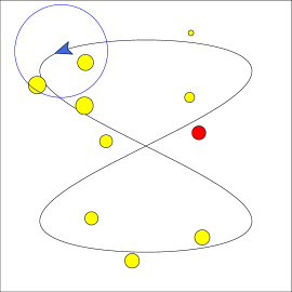
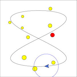
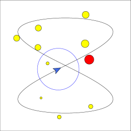
Figure 4: An example with a field consisting of $10$ points. The field $Z(\mathbf{q},t)$ at each point is indicated by the area of the disk centered at the point. The vehicle footprint is a disk. The time sequence of the three snapshots goes from left to right. The vehicle is moving counter-clockwise around the top half of the figure eight and clockwise around the bottom half. The time evolution of the red field point is shown in Figure 5.

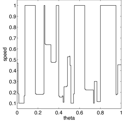
(a) The optimal speed controller.

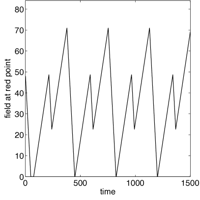
(b) The field $Z(\mathbf{q},t)$ at the red (dark) point.

Figure 5: The optimal speed controller corresponding to the curve and field shown in Figure 4. The minimum speed is $v_{\min}=0.22~{}\mathrm{m/s}$ and the maximum speed is $v_{\max}=2~{}\mathrm{m/s}$. The field $Z(\mathbf{q},t)$ is shown for the red (dark) point in Figure 4. It converges in finite time to a steady state.

The field $Z(\mathbf{q},t)$ for the red (shaded) point in Figure 4, is shown as a function of time in Figure 5b. One can see that the field converges in finite time to a periodic cycle. In addition, the field goes to zero during each cycle. The periodic cycle is the steady-state as characterized in Section III-B.

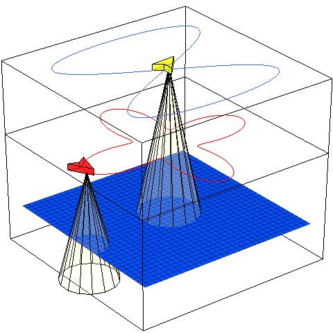
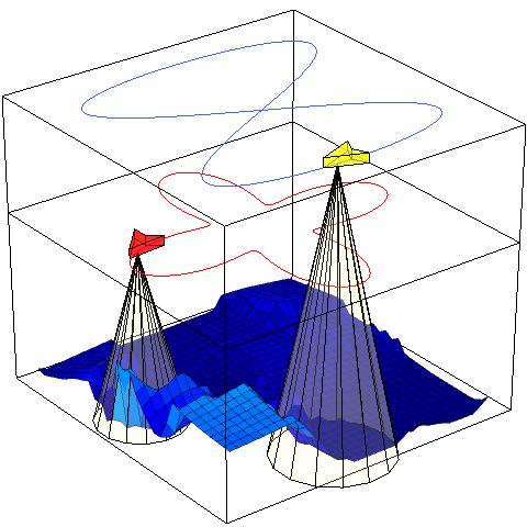
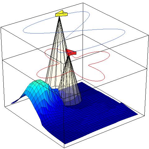
Figure 6: An example of using a discretized approximation of a continuous field for two robots. The grid is $32\times 32$, and the field $Z(\mathbf{q},t)$ at each point is shown as the surface. The footprint of the higher robot (yellow) is $4/3$ the radius of the footprint of the lower (red) robot. The snapshot sequence goes from left to right with the left snapshot showing the initial condition of the robots and field.

In Figure 6, a simulation is shown for the case when the entire continuous environment must be monitored by two aerial robots. For multiple robots we synthesized a field stabilizing controller by maximizing the stability margin, as discussed in Remark IV.5. The continuous field is defined over a $690~{}\mathrm{m}$ by $690~{}\mathrm{m}$ square, and was approximated using a $32\times 32$ grid. For all points $\mathbf{q}\in Q$ we set the consumption rate $c(\mathbf{q})=1$, and the production function is shown in Figure 7.

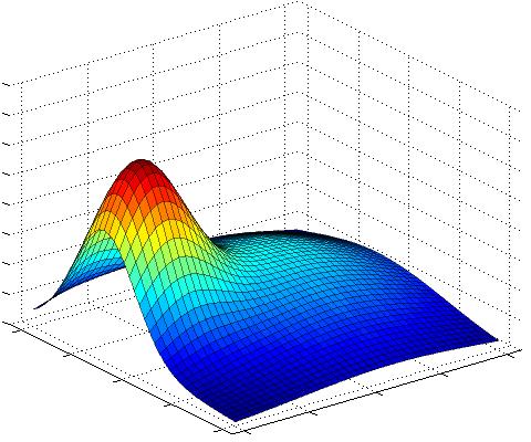
Figure 7: The production function $p(\mathbf{q})$ for the simulations in Figures 8 and 6.

Robot $1$ followed a figure-eight path which has a length of $2630~{}\mathrm{m}$, while robot $2$ followed a four-leaf clover path with a length of $2250~{}\mathrm{m}$. The footprint for robot $1$, the higher (yellow) robot had a radius of $100~{}\mathrm{m}$, and the speed constraints were given by $v_{\min,1}=1.5~{}\mathrm{m/s}$ and $v_{\max,1}=15~{}\mathrm{m/s}$. The footprint for robot $2$, the lower (red) robot, had a radius of $133~{}\mathrm{m}$, and the speed constraints were given by $v_{\min,2}=2~{}\mathrm{m/s}$ and $v_{\max,2}=20~{}\mathrm{m/s}$. The cycle time for robot $1$ was $T_{1}=519~{}\mathrm{s}$, and the cycle time for robot $2$ was $T_{2}=443~{}\mathrm{s}$. A total of $150$ rectangular basis functions were used for each robot’s speed controller. The optimization was solved in approximately $10$ seconds. A snapshot for a simulation with three robots is shown in Figure 1. In this case, the green robot flying at a higher altitude has a square footprint which is oriented with the robot’s current heading.

V-A A Case Study in Robustness

In this subsection we demonstrate how we can compute a speed controller that exhibits robustness to motion errors, modeling uncertainty, or stochastic fluctuations. This is important since the speed controller is computed offline. It should be noted, however, that in practice the controller can be recomputed periodically during the robot’s execution, taking into account new information about the field evolution.

As shown in Corollary III.2 we can maximize stability margin of a speed controller. The corollary showed that in maximizing this metric we obtain some robustness to error. To explore the robustness properties of this controller, consider the single robot example in Figure 8. In this example, the square $665~{}\mathrm{m}$ by $665~{}\mathrm{m}$ environment must be monitored by an aerial robot. We approximated the continuous field using a $32\times 32$ grid. The consumption rate was set to $c(\mathbf{q})=5$, for each field point $\mathbf{q}\in Q$. The production rate of the field was given by the function shown in Figure 7. The maximum production rate of the field was $0.74$ and the average was $0.21$. The robot had a circular footprint with a radius of $133~{}\mathrm{m}$, a minimum speed of $v_{\min}=1.5~{}\mathrm{m/s}$ and a maximum speed of $v_{\max}=15~{}\mathrm{m/s}$. The path had a cycle length of $4200~{}\mathrm{m}$. If the robot followed the path at constant speed, then $80$ of the points would be unstable.

For the speed controller, we used $280$ rectangular basis functions, and solved the optimization as described in Corollary III.2, resulting in a stability margin of $B=97.8$. The optimization was solved in approximately $10$ seconds. The time for the robot to complete one cycle of the path using this controller was $T=439~{}\mathrm{s}$.

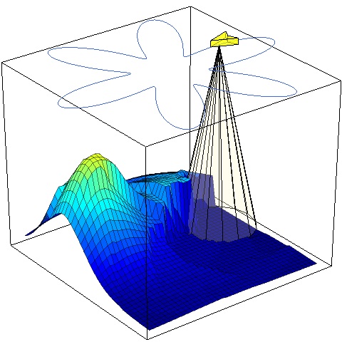
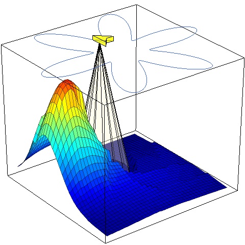
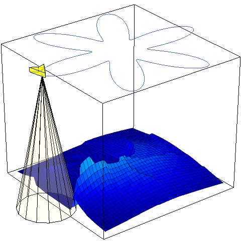
Figure 8: An example of using a discretized approximation of a continuous field. The field $Z(\mathbf{q},t)$ at each point is shown as the surface. The footprint of the vehicle is a disk, and the robot’s trajectory is given by the “six leaf” clover. The time sequence of the three snapshots goes from left to right. In the rightmost snapshot the vehicle has just finished reducing the large peak that forms in the left and center snapshots.

Stochastic field evolution: Now, suppose that we add zero-mean noise to the production function. Thus, the robot based its speed controller on the “nominal” production function $\bar{p}(\mathbf{q})$ (shown in Figure 7), but the actual production function is $p(\mathbf{q},t)=\bar{p}(\mathbf{q})+n(t,\mathbf{q})$, where $n(t,\mathbf{q})$ is noise. For the simulation, at each time instant $t$, and for each point $\mathbf{q}\in Q$, we independently draw $n(t,\mathbf{q})$ uniformly from the set $[-n_{\max},n_{\max}]$, where $n_{\max}>0$ is the maximum value of the noise.

The simulations were carried out as follows. We varied the magnitude of the noise $n_{\max}$, and studied the maximum value reached by the field. For each value $n_{\max}$, we performed $20$ trials, and in each trial we recorded the maximum value reached by the field on a time horizon of $2500~{}\mathrm{s}$. In Figure 9, we display statistics from the $20$ independent trials at each noise level, namely the mean, minimum, and maximum, as well as the standard deviation. With zero added noise, one can see that the mean, minimum, and maximum all coincide. As noise is added to the evolution, the difference between the minimum and maximum value grows. However, it is interesting to note that while the performance degrades (i.e., the mean increases with increasing noise), the system remains stable. Thus, the simulation demonstrates some of the robustness properties of the proposed controller.

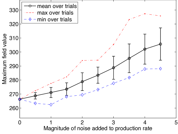
Figure 9: The robustness of the speed controller to noise in the production rate. For each value of noise $n_{\max}$, the plot shows statistics on the maximum value reached by the field over 20 independent trials.

Parameter errors: We can also consider robustness to parameter errors. In particular, consider the case where the robot bases its optimization on a production rate of $\bar{p}(\mathbf{q})$ (shown in Figure 7), but the actual production rate is given by $p(\mathbf{q})=\bar{p}(\mathbf{q})+\epsilon$, where $\epsilon>0$ (note that the field is trivially stable for any $\epsilon\leq 0$). By maximizing the stability margin, we obtain some level of robustness against this type of parameter uncertainty. The amount of error that we can tolerate is directly related to the stability margin $B=97.8$, as shown in Corollary III.2. In particular, we obtain $\epsilon<Bc(\mathbf{q}_{i})/\big{(}\sum_{j=1}^{n}\alpha_{j}\int_{0}^{1}\beta_{j}(\theta)d\theta\big{)}=0.074$. We performed simulations of monitoring task for successively larger values of $\epsilon$. From this data, we verified that the field remains stable for any $\epsilon\leq 0.07$. For this example, the average value of $p(\mathbf{q})$ over all points $\mathbf{q}$ is $0.21$, and so we can handle uncertainty in the magnitude of the production rate on the order of $30\%$.

Tracking error: After running the speed optimization, a robot has a desired trajectory, consisting of the pre-specified path and the optimized speed along the path. In practice, this trajectory will be the input to a tracking controller, which takes into account the robot dynamics. Since there are inevitably tracking errors, the stability margin of the controller is needed to ensure field stability. As an example, we considered a unicycle model for an aerial robot. In this model, the robot’s configuration is given by a heading $\phi$ and a position $(x,y)$. The control inputs are the linear and angular speeds: $\dot{x}=v\cos\phi$, $\dot{y}=v\sin\phi$, and $\dot{\phi}=\omega$. The linear speed had bounds of $v_{\min}=1.5~{}\mathrm{m/s}$ and $v_{\max}=15~{}\mathrm{m/s}$, and the angular speed was upper bounded by $0.5~{}\mathrm{rad/s}$. We used the same speed controller as in the previous two examples (maximizing the stability margin). For trajectory tracking, we used a dynamic feedback linearization controller [39]. We chose conservative controller gains of $0.5$ for the proportional and derivative control in order to accentuate the tracking error. The results are shown in Figure 10. Due to the stability margin of $97.8$, the field remains stable, even in the presence of this tracking error. However, in simulation, the maximum field height increased by about $13\%$ from $268$ (as shown for the zero noise case in Figure 9) to $305$.

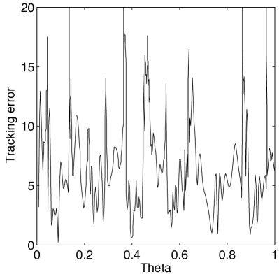
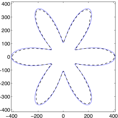
Figure 10: The robustness of the speed controller to tracking errors. The left figure shows the absolute tracking error in meters. In the right figure, the solid line is the desired path, and the dashed line is the path executed by the unicycle robot.

VI Conclusions, Extensions, and Open Problems

In this paper we proposed a model for persistent sweeping and monitoring tasks and derived controllers for robots to accomplish those tasks. We specifically considered the case in which robots are confined to pre-specified, closed paths, along which their speed must be controlled. We formulated an LP whose solution gives speed controllers that keep the accumulation bounded everywhere in the environment for single robots and multiple robots. For single robots, we also formulated a different LP to give the optimal controller—the one that keeps the accumulation function as low as possible everywhere. We see this as a solution to one kind of persistent task for robots, but many open problems remain.

VI-A Extensions and Open Problems

We are interested in the general problem of solving persistent tasks, which we broadly define as tasks that require perpetual attention by a robotic agent. The main objective of a persistent task is to maintain the accumulation of some undesirable quantity at as low a value as possible over an environment using one or multiple robotic agents. The difficulty of this problem depends on what is known by the robots, and precisely what the robots’ capabilities are. Let us enumerate several possible dimensions for extension on this problem.

• Trajectory vs. Path vs. Speed One might consider controlling only the speed over a prescribed path, as we have done in this paper, only the path with a prescribed speed, or complete trajectory planning.

• Single vs. Multiple Robots There may be only one robot, or there may be a team of robots, potentially with heterogeneous capabilities and constraints.

• Known vs. Unknown Production Rate The robot may know (or be able to sense) the production rate, or it may have to learn it over time from measurements.

• Constant vs. Time-Varying Production Rate The production rate may be constant in time, or it may change indicating a change in the environment’s dynamics.

• Finite vs. Continuum Points of Interest The points of interest in the environment may be viewed as a finite set of discrete points over which to control the accumulation, or as an infinite continuum in which we would like to control the accumulation at every point.

In this paper we specifically considered speed control over a prescribed path of both single and multiple robots in a finite environment with a known, constant production rate.

One interesting direction in which to expand this work is to consider planning full trajectories for robots to carry out persistent tasks. The high dimensionality of the space of possible trajectories makes this a difficult problem. However, if the robot’s path is limited by some inherent constraints, then this problem may admit solutions with guarantees. For example, underwater gliders are commonly constrained to take piecewise linear paths, which can be parametrized with a low number of parameters. Another direction of extension is to have a robot solve the LP for its controller on-line. This would be useful if, for example the production rate is not known before hand, but can be sensed over the sensor footprint of the robot. Likewise if the production rate changes in time, it would be useful for a robot to be able to adjust its controller on-line to accommodate these changes. A promising approach for this is to repeatedly solve for the LP in a receding horizon fashion, using newly acquired information to update the model of the field evolution. We continue to study problems of persistent tasks for robots in these and other directions.

[Periodic Position-Feedback Controllers]

In this appendix we will prove Proposition II.4 on periodic position-feedback controllers.

Consider a general speed controller $(Z,\mathrm{IC},t)\mapsto v(\theta,Z,\mathrm{IC},t)$ where $\mathrm{IC}:=(Z(\mathbf{q},0),\theta(0))$ is the set of initial conditions. Since $v_{\min}(\theta)>0$ for all $\theta\in[0,1]$, the value of $\theta$ strictly monotonically increases from $0$ to $1$ for every valid controller (once it reaches $1$ it then wraps around to $0$). In addition, the evolution of $Z$ is deterministic and is uniquely determined by the initial conditions and the speed controller, as given in (1). Because of this, every controller of the form $v(\theta,Z,\mathrm{IC},t)$ can be written as an infinite sequence of controllers $v_{1}(\theta,\mathrm{IC}),v_{2}(\theta,\mathrm{IC}),\ldots$, where controller $v_{k}(\theta,\mathrm{IC})$ is the controller used during the $k$th period (or cycle).

With the above discussion in place, we are now ready to prove Proposition II.4

Proof of Proposition II.4.

To begin, consider a feasible persistent monitoring task and a field stabilizing controller of the form $v(\theta,Z,\mathrm{IC},t)$, where $\mathrm{IC}:=(Z(\mathbf{q},0),\theta(0))$. Without loss of generality, we can assume that $\theta(0):=0$. From the discussion above, we can write the general controller as a sequence of controllers $v_{1}(\theta,\mathrm{IC}),v_{2}(\theta,\mathrm{IC}),\ldots$, where controller $v_{k}(\theta,\mathrm{IC})$, $k\in\mathbb{N}$ is used on the $k$th period (or cycle).

Since the controller is stable, there exists a $Z_{\max}$ such that for every set of initial conditions $\mathrm{IC}$, we have $\limsup_{t\to+\infty}Z(\mathbf{q},t)\leq Z_{\max}$. Let us fix $\epsilon>0$ and fix the initial conditions to a set of values $\overline{\mathrm{IC}}$ such that $Z(\mathbf{q},0)>Z_{\max}+\epsilon$ for all $\mathbf{q}\in Q$. Now, we will prove the result by constructing a periodic position-feedback controller.

Let $t_{1}=0$ and define

$$t_{k}=t_{k-1}+\int_{0}^{1}\frac{1}{v_{k}(\theta,\overline{\mathrm{IC}})}d\theta,$$

for each integer $k\geq 2$. Thus, controller $v_{k}$ is used during the time interval $[t_{k},t_{k+1}]$. Following the same argument as in the proof of Lemma II.5, we have that for each $\mathbf{q}\in Q$,

$$Z(\mathbf{q},t_{k})-Z(\mathbf{q},t_{1})\geq p(\mathbf{q})\sum_{\ell=1}^{k}\int_{0}^{1}\frac{1}{v_{\ell}(\theta,\overline{\mathrm{IC}})}d\theta\\ -c(\mathbf{q})\sum_{\ell=1}^{k}\int_{F(\mathbf{q})}\frac{1}{v_{\ell}(\theta,\overline{\mathrm{IC}})}d\theta.$$

Now, $Z(\mathbf{q},t_{1})>Z_{\max}+\epsilon$ is the initial condition, and $\limsup_{t\to+\infty}Z(\mathbf{q},t)\leq Z_{\max}$. Thus, for every fixed $\delta\in(0,\epsilon)$, there exists a finite $k$ such that $Z(\mathbf{q},t_{k})\leq Z_{\max}+\delta$. Since this must hold for every $\mathbf{q}\in Q$, we see that there exists an integer $k$ such that

$$p(\mathbf{q})\sum_{\ell=1}^{k}\int_{0}^{1}\frac{1}{v_{\ell}(\theta,\overline{\mathrm{IC}})}d\theta-c(\mathbf{q})\sum_{\ell=1}^{k}\int_{F(\mathbf{q})}\frac{1}{v_{\ell}(\theta,\overline{\mathrm{IC}})}d\theta<0,$$

for every $\mathbf{q}\in Q$. Rearranging the previous equation we obtain

$$c(\mathbf{q})\int_{F(\mathbf{q})}\sum_{\ell=1}^{k}\frac{1}{v_{\ell}(\theta,\overline{\mathrm{IC}})}d\theta>p(\mathbf{q})\int_{0}^{1}\sum_{\ell=1}^{k}\frac{1}{v_{\ell}(\theta,\overline{\mathrm{IC}})}d\theta.$$ (24)

Therefore, let us define the periodic controller

$$v(\theta)=k\left(\sum_{\ell=1}^{k}\frac{1}{v_{\ell}(\theta,\overline{\mathrm{IC}})}\right)^{-1},$$

for each $\theta\in[0,1]$. Note that if $v_{\min}(\theta)\leq v_{\ell}(\theta,\overline{\mathrm{IC}})\leq v_{\max}(\theta)$ for all $\theta\in[0,1]$ and all $\ell\in\mathbb{N}$, then

$$v_{\min}(\theta)\leq v(\theta)\leq v_{\max}(\theta).$$

But, combining the definition of $v(\theta)$ with (24), we immediately see that $v(\theta)$ satisfies the stability condition in Lemma II.5, and thus $v(\theta)$ is a field stabilizing position-feedback controller. ∎

References

- [1] N. M. P. Kakalis and Y. Ventikos, “Robotic swarm concept for efficient oil spill confrontation,” Journal of Hazardous Materials, vol. 154, pp. 880–887, 2008.
- [2] D. MacKenzie and T. Balch, “Making a clean sweep: Behavior-based vacuuming,” in Proceedings of the AAAI Fall Symposium: Instantiating Real-world Agents, Raleigh, NC, March 1993.
- [3] N. Correll, N. Arechiga, A. Bolger, M. Bollini, B. Charrow, A. Clayton, F. Dominguez, K. Donahue, S. Dyar, L. Johnson, H. Liu, A. Patrikalakis, T. Robertson, J. Smith, D. Soltero, M. Tanner, L. White, and D. Rus, “Building a distributed robot garden,” in IEEE/RSJ Int. Conf. on Intelligent Robots & Systems, St. Louis, MO, 2009, pp. 1509–1516.
- [4] R. N. Smith, M. Schwager, S. L. Smith, B. H. Jones, D. Rus, and G. S. Sukhatme, “Persistent ocean monitoring with underwater gliders: Adapting spatiotemporal sampling resolution,” Journal of Field Robotics, 2010, Submitted.
- [5] M. Dunbabin, J. Roberts, K. Usher, and P. Corke, “A new robot for environmental monitoring on the Great Barrier Reef,” in Australasian Conference on Robotics and Automation, Australian National University, Canberra, December 2004.
- [6] S. Srinivasan, H. Latchman, J. Shea, T. Wong, and J. McNair, “Airborne traffic surveillance systems: video surveillance of highway traffic,” in International workshop on Video Surveillance & Sensor Networks, New York, NY, USA, October 2004, pp. 131–135.
- [7] S. L. Smith and D. Rus, “Multi-robot monitoring in dynamic environments with guaranteed currency of observations,” in IEEE Conf. on Decision and Control, Atlanta, GA, Dec. 2010, pp. 514–521.
- [8] K. Kant and S. W. Zucker, “Toward efficient trajectory planning: The path-velocity decomposition,” International Journal of Robotics Research, vol. 5, no. 3, pp. 72–89, 1986.
- [9] D. G. Luenberger, Linear and Nonlinear Programming, 2nd ed. Addison-Wesley, 1984.
- [10] E. W. Cheney, Introduction to Approximation Theory, 2nd ed. AMS Chelsea Publishing, 2000.
- [11] E. J. Candes and M. B. Wakin, “An introduction to compressive sampling,” IEEE Signal Processing Magazine, pp. 21–30, Mar. 2008.
- [12] R. Sanner and J. Slotine, “Gaussian networks for direct adaptive control,” IEEE Transactions on Neural Networks, vol. 3, no. 6, pp. 837–863, 1992.
- [13] T. Poggio and S. Smale, “The mathematics of learning: Dealing with data,” Notices of the American Mathematical Society, vol. 50, no. 5, pp. 537–544, 2003.
- [14] L. S. Gandin, Objective Analysis of Meteorological Fields. Jerusalem: Israeli Program for Scientific Translations, 1966, (originally published in Russian in 1963, Gidrometeor, Leningrad).
- [15] N. Cressie, “The origins of kriging,” Mathematical Geology, vol. 22, no. 3, pp. 239–252, 1990.
- [16] B. Grocholsky, “Information-theoretic control of multiple sensor platforms,” Ph.D. dissertation, University of Sydney, 2002.
- [17] K. M. Lynch, I. B. Schwartz, P. Yang, and R. A. Freeman, “Decentralized environmental modeling by mobile sensor networks,” IEEE Transactions on Robotics, vol. 24, no. 3, pp. 710–724, June 2008.
- [18] P. Yang, R. A. Freeman, and K. M. Lynch, “Mulit-agent coordination by decentralized estimation and control,” IEEE Transactions on Automatic Control, vol. 53, no. 11, pp. 248–2496, December 2008.
- [19] J. Cortés, “Distributed Kriged Kalman filter for spatial estimation,” IEEE Transactions on Automatic Control, vol. 54, no. 12, pp. 2816–2827, 2009.
- [20] F. Zhang and N. E. Leonard, “Cooperative filters and control for cooperative exploration,” IEEE Transactions on Automatic Control, vol. 55, no. 3, pp. 650–663, 2010.
- [21] R. Graham and J. Cortés, “Adaptive information collection by robotic sensor networks for spatial estimation,” IEEE Transactions on Automatic Control, 2010, Submitted.
- [22] J. L. Ny and G. J. Pappas, “On trajectory optimization for active sensing in gaussian process models,” in IEEE Conf. on Decision and Control and Chinese Control Conference, Shanghai, China, December 2009, pp. 6282–6292.
- [23] F. Bourgault, A. A. Makarenko, S. B. Williams, B. Grocholsky, and H. F. Durrant-Whyte, “Information based adaptive robotic exploration,” in IEEE/RSJ Int. Conf. on Intelligent Robots & Systems, 2002, pp. 540–545.
- [24] E. M. Arkin, S. P. Fekete, and J. S. B. Mitchell, “Approximation algorithms for lawn mowing and milling,” Computational Geometry: Theory and Applications, vol. 17, no. 1-2, pp. 25–50, 2000.
- [25] I. Rekleitis, V. Lee-Shue, A. P. New, and H. Choset, “Limited communication multi-robot team based coverage,” in IEEE Int. Conf. on Robotics and Automation, New Orleans, LA, Apr. 2004, pp. 3462–3468.
- [26] S. Koenig, B. Szymanski, and Y. Liu, “Efficient and inefficient ant coverage methods,” Annals of Mathematics and Artificial Intelligence, vol. 31, pp. 41–76, 2001.
- [27] H. Choset, “Coverage for robotics – A survey of recent results,” Annals of Mathematics and Artificial Intelligence, vol. 31, no. 1-4, pp. 113–126, 2001.
- [28] B. Bethke, J. P. How, and J. Vian, “Group health management of UAV teams with applications to persistent surveillance,” in American Control Conference, Seattle, WA, Jun. 2008, pp. 3145–3150.
- [29] B. Bethke, J. Redding, J. P. How, M. A. Vavrina, and J. Vian, “Agent capability in persistent mission planning using approximate dynamic programming,” in American Control Conference, Baltimore, MD, Jun. 2010, pp. 1623–1628.
- [30] Y. Chevaleyre, “Theoretical analysis of the multi-agent patrolling problem,” in IEEE/WIC/ACM Int. Conf. Intelligent Agent Technology, Beijing, China, Sep. 2004, pp. 302–308.
- [31] Y. Elmaliach, N. Agmon, and G. A. Kaminka, “Multi-robot area patrol under frequency constraints,” in IEEE Int. Conf. on Robotics and Automation, Roma, Italy, Apr. 2007, pp. 385–390.
- [32] N. Nigram and I. Kroo, “Persistent surveillance using multiple unmannded air vehicles,” in IEEE Aerospace Conf., Big Sky, MT, May 2008, pp. 1–14.
- [33] D. B. Kingston, R. W. Beard, and R. S. Holt, “Decentralized perimeter surveillance using a team of UAVs,” IEEE Transactions on Robotics, vol. 24, no. 6, pp. 1394–1404, 2008.
- [34] P. F. Hokayem, D. Stipanović, and M. W. Spong, “On persistent coverage control,” in IEEE Conf. on Decision and Control, New Orleans, LA, Dec. 2007, pp. 6130–6135.
- [35] L. Kleinrock, Queueing Systems. Volume I: Theory. John Wiley, 1975.
- [36] D. J. Bertsimas and G. J. van Ryzin, “Stochastic and dynamic vehicle routing in the Euclidean plane with multiple capacitated vehicles,” Operations Research, vol. 41, no. 1, pp. 60–76, 1993.
- [37] S. L. Smith, M. Pavone, F. Bullo, and E. Frazzoli, “Dynamic vehicle routing with priority classes of stochastic demands,” SIAM Journal on Control and Optimization, vol. 48, no. 5, pp. 3224–3245, 2010.
- [38] M. Ahmadi and P. Stone, “A multi-robot system for continuous area sweeping tasks,” in IEEE Int. Conf. on Robotics and Automation, Orlando, FL, May 2006, pp. 1724–1729.
- [39] G. Oriolo, A. D. Luca, and M. Vendittelli, “WMR control via dynamic feedback linearization: design, implementation, and experimental validation,” IEEE Transactions on Control Systems Technology, vol. 10, no. 6, pp. 835–852, 2002.