Survival of scalar zero modes in warped extra dimensions

Abstract

Models with an extra dimension generally contain background scalar fields in a non-trivial configuration, whose stability must be ensured. With gravity present, the extra dimension is warped by the scalars, and the spin-0 degrees of freedom in the metric mix with the scalar perturbations. Where possible, we formally solve the coupled Schrödinger equations for the zero modes of these spin-0 perturbations. When specialising to the case of two scalars with a potential generated by a superpotential, we are able to fully solve the system. We show how these zero modes can be used to construct a solution matrix, whose eigenvalues tell whether a normalisable zero mode exists, and how many negative mass modes exist. These facts are crucial in determining stability of the corresponding background configuration. We provide examples of the general analysis for domain-wall models of an infinite extra dimension and domain-wall soft-wall models. For 5D models with two scalars constructed using a superpotential, we show that a normalisable zero mode survives, even in the presence of warped gravity. Such models, which are widely used in the literature, are therefore phenomenologically unacceptable.

I Introduction

A plausible way to extend the standard model is to embed it in one or more extra dimensions. This opens up a new set of model-building tools which can help to solve a diverse range of theoretical and phenomenological problems, as well as yielding distinct collider signatures such as Kaluza-Klein (KK) modes. Almost all extra-dimensional models require one or more background scalar fields in some non-trivial configuration. For example, to generate a domain-wall which localises chiral fermions Rubakov and Shaposhnikov (1983), to stabilise the size of a compact extra dimension Goldberger and Wise (1999); Csaki et al. (2001), to generalise the Randall-Sundrum warped-space Randall and Sundrum (1999) to a smoothed-out version Csaki et al. (2000), or to cut off the extra dimension at a singularity Gremm (2000); Karch et al. (2006). Domain-wall models, whether they have an infinite Davies et al. (2008) or compact Aybat and George (2010) extra dimension, make heavy use of background scalar configurations as a field-theoretic substitution for fundamental branes.

Given the ubiquity and necessity of background scalar fields, it is important to understand both their statics and dynamics. The problem is best thought about in terms of a ground state, upon which exist perturbations. We want to know which particular scalar configurations have the lowest energy and are stable, and what the perturbations about a background lead to in terms of effective 4D modes. These two issues are closely related. The existence of negative-mass modes (tachyonic KK modes) signals an instability of the corresponding background. Massless modes may also signal an instability Aybat and George (2010), or be harmless in the case of a translation mode. Positive-mass modes always exist and their precise spectrum is what distinguishes these extra-dimensional models at a particle collider.

For the case of a single scalar field in a flat compact extra dimension, a general method for determining the lowest energy configuration has been worked out Toharia and Trodden (2008a, b). The inclusion of gravity in the analysis presents some complications because of the coupling of the scalar fields to gravity. This coupling generically warps the extra dimension Csaki et al. (2000) and the scalar perturbations mix with the spin-0 degrees of freedom in the metric. For this warped case with one extra dimension there have been some general stability analyses with a single background scalar Kobayashi et al. (2002); Toharia (2008), and some initial work on the multiple scalar case Toharia et al. (2010); Aybat and George (2010). For the case of a single scalar in multiple extra dimensions it has also been shown that the scalar and metric spin-0 modes mix Underwood (2011). Related analyses determining the spin-0 spectrum of multiple scalars in 5D have been done in the context of the AdS/CFT correspondence Berg et al. (2006, 2008); Elander (2010). In particular, an algorithm for computing the scalar spectrum in general 5D compact models has been prescribed Elander and Piai (2011).

Despite the complications introduced by gravity, it is still possible to find the effective coupled Schrödinger equations which describe the KK modes of multiple scalars in a warped background Aybat and George (2010). It is the aim of the current paper to, when possible, formally solve this set of Schrödinger equations for the massless KK modes — the zero modes — in the case of a 5D bulk with no gravity (flat) and with gravity (warped). In addition to providing closed form solutions for the zero modes for a large number of cases, we shall also discuss how these solutions can be used to determine if any normalisable zero modes exist and whether or not the background is perturbatively stable. Some relevant examples shall be provided.

One reason for studying the zero modes of the system is that, if they exist, they should play a large role at low energies in the effective 4D theory. For example, zero modes of a 5D fermion are generally used to implement the fermions of the standard model Davies et al. (2008). When constructing domain-wall models using scalar background fields in flat space, one always obtains a spin-0 zero mode corresponding to the broken translation symmetry. This degree of freedom is not welcome in the effective 4D theory since we have never observed such a particle, which would manifest as a “fifth force”. Adding warped gravity can cure this problem since this removes the translation zero mode, as shown by Shaposhnikov et. al. Shaposhnikov et al. (2005) for the case of a single background scalar. In this paper this result is extended to the case of multiple background scalar fields: the zero mode of translation does not survive, no matter how many scalars. It is possible though, and we shall give some explicit examples, that additional scalars introduce additional zero modes which do survive in the presence of gravity. Our examples of such models are constructed using the superpotential approach, and we argue that these models are phenomenologically unacceptable.

The paper is organised as follows. In Section II we first present the zero mode solutions, for the flat and warped cases, with general potential $V$ and also specialising to a superpotential $W$ with $N=2$ scalars. For this latter case we give all four independent zero modes in closed analytic form. Section III discusses the construction of a solution matrix, and how its eigenvalues can be used to find normalisable zero modes, and count the number of normalisable negative modes. Following this we look in Sections IV and V at specific domain-wall models in both an infinite and a compact extra dimension, and show that zero modes can survive in the presence of gravity. We conclude in Section VI. Appendix A summarises the method of reduction of order for ordinary differential equations.

II The zero mode solutions

In this section we study spin-0 perturbations of $N$ real scalar fields in a 5D bulk for both a flat and warped extra dimension. The scalar fields are assumed to have some non-trivial background profile along the extra dimension, such as a kink. The aim is to derive formal solutions for the extra-dimensional profile of the zero modes, that is, the massless perturbations around the background. We shall concentrate mainly on the $N=2$ case, and, for part of the analysis, specialise to potentials $V$ that are generated by a superpotential $W$.

Throughout this paper we work with the matter Lagrangian

$$\mathcal{L}_{m}=-\frac{1}{2}g^{MN}\partial_{M}\Phi_{i}\partial_{N}\Phi_{i}-V(\Phi_{i})\>,$$ (1)

where $g_{MN}$ is the 5D metric with signature $(-++++)$, $\Phi_{i}(x^{\mu},y)$ are $N$ scalar fields indexed by $i=1\ldots N$, $x^{\mu}$ is the 4D sub-spacetime, $y$ is the coordinate of the extra dimension, and $V(\Phi_{i})$ is the scalar potential. Repeated scalar field indices are always summed over. Perturbations of the scalar fields around some arbitrary background are written as

$$\Phi_{i}(x^{\mu},y)=\phi_{i}(y)+\varphi_{i}(x^{\mu},y)\>.$$ (2)

The background profiles $\phi_{i}(y)$ depend only on the extra dimension, while the perturbations are general functions of all spacetime coordinates, and are required to be relatively small: $\varphi_{i}\ll\phi_{i}$.

From the equations of motion for the scalars one can obtain $N$ coupled, one dimensional, time-independent Schrödinger-like equations for the perturbations. The independent variable of the these equations is the extra dimension $y$ and the eigenvalue corresponds to the mass of the KK mode of the perturbation. Where possible, we shall formally solve this system of coupled Schrödinger equations for the case of a zero eigenvalue. Since we have $N$ second order, linear, ordinary differential equations (ODEs) we expect to obtain $2N$ linearly independent solutions. These $2N$ solutions are not necessarily physical (that is, are not normalisable), but they do form a basis from which one can construct the unique solution for any given initial, boundary and/or normalisability conditions. The zero mode solutions are useful for studying the perturbative stability of the background configuration, as shall be discussed in Section III.

II.1 Flat case

We analyse first the gravity-free, flat-space scenario where the action is given simply by $\mathcal{S}=\int\mathcal{L}_{m}\,d^{4}x\,dy$. The discussion is divided into the case of a general $V$, and the case where $V$ is generated by a (fake) superpotential $W$.

II.1.1 General $V$

In flat space, the general background equations are

$$\phi_{i}^{\prime\prime}-V_{i}=0\>,$$ (3)

and the coupled Schrödinger-like equations for the perturbations are

$$-\varphi_{i}^{\prime\prime}+V_{ij}\varphi_{j}=\Box\varphi_{i}\>.$$ (4)

Prime denotes derivative with respect to $y$, subscripts $i$ and $j$ on $V$ denote a derivative with respect to $\Phi_{i}$ and $\Phi_{j}$, and $\Box=\partial^{\mu}\partial_{\mu}$. In addition, $V_{ij}$, which is a function of $\Phi_{i}$, must be evaluated on the background solution, $\Phi_{i}=\phi_{i}(y)$, where $\phi_{i}(y)$ is a solution to equation (3). As usual, separation of variables of $x^{\mu}$ and $y$ is the correct way to proceed here. For the sake of reducing the number of field variables we shall abuse notation slightly by using $\varphi_{i}$ to denote both the full perturbation which is a function of $x^{\mu}$ and $y$, as well as the separated factor that depends only on $y$. Separation of variables then proceeds as per $\varphi_{i}(x^{\mu},y)=\varphi_{i}(y)\rho(x^{\mu})$, with $\rho$ the 4D KK mode with mass $m$, such that $\Box\rho=m^{2}\rho$.

One now solves equation (4) for the profiles $\varphi_{i}(y)$ and corresponding allowed mass values, obtaining a tower of modes. Then one takes the original 5D action and substitutes $\Phi_{i}=\phi_{i}(y)+\varphi_{i}(y)\rho(x^{\mu})$ with $\varphi_{i}(y)$ a particular solution. The extra dimension can then be integrated out, leaving an effective 4D action for the mode $\rho$. To second order in $\rho$, this action is

$$\mathcal{S}=\int d^{4}x\left[-\varepsilon_{\text{bg}}+\mathcal{N}\left(-\frac{1}{2}\partial^{\mu}\rho\partial_{\mu}\rho-\frac{1}{2}m^{2}\rho^{2}\right)\right]+\text{(surface terms)}\>.$$ (5)

Here, $\varepsilon_{\text{bg}}$ is the energy density of the scalar background configuration. The normalisation constant for the mode is $\mathcal{N}=\int\varphi_{i}^{2}dy$ and, so long as we pick a solution $\varphi_{i}$ that is normalisable, one can scale said solution to obtain $\mathcal{N}=1$. The action then describes a canonical, 4D scalar field. The surface terms in the action are of the form $\int S^{\prime}d^{4}x\,dy$, where $S$ is one of

$$S_{1} =-\phi_{i}^{\prime}\varphi_{i}\>,$$ (6a)

$$S_{2} =-\frac{1}{2}\varphi_{i}\varphi_{i}^{\prime}\>.$$ (6b)

The requirements that these terms independently vanish on the boundaries of the extra dimension, and that $\mathcal{N}$ is finite, pick out the physical modes of the KK tower.

As mentioned previously, we are interested in the zero modes, and shall look for formal solutions to equation (4) when $\Box\varphi_{i}=0$. For general $V$ and all $N$ one solution is

$$\varphi_{i}^{(1)}=\phi_{i}^{\prime}\>,$$ (7)

where $\phi_{i}$ is the background scalar field configuration. Note that this solution is actually a vector of length $N$. It is the well-known translation mode of the background, since it is the first term in a Taylor expansion of the shifted background: $\phi_{i}(y+\epsilon)=\phi_{i}(y)+\epsilon\phi_{i}^{\prime}(y)+\mathcal{O}(\epsilon^{2})$. For the case of $N=1$, where there are $2N=2$ independent solutions, we can use the $\varphi_{i}^{(1)}$ solution to perform reduction of order (see Appendix A) and obtain the other solution:

$$\varphi_{i}^{(2,N=1)}=\phi^{\prime}\int\left(\phi^{\prime}\right)^{-2}dy\>.$$ (8)

For $N>1$ we could also perform reduction of order, but we would still have a relatively large (at least third order for $N=2$) ODE to solve. At this point we shall be content with having only the translation solution for general $N$.

II.1.2 $V$ generated by a superpotential

It is possible to make progress and obtain an additional zero mode solution when the form of $V$ is restricted to

$$V=\frac{1}{2}W_{i}^{2}\>,$$ (9)

where $W(\Phi_{i})$ is a fake superpotential (it is just a formal construction and does not indicate a supersymmetry). As it does on $V$, a subscript $i$ on $W$ denotes a derivative with respect to $\Phi_{i}$. In this case the background equations can be written as

$$\phi_{i}^{\prime}=W_{i}\>,$$ (10)

and the perturbation equation (4) becomes

$$-\varphi_{i}^{\prime\prime}+(W_{ij}W_{jk}+W_{ijk}W_{j})\varphi_{k}=\Box\varphi_{i}\>.$$ (11)

Here, $W_{ij}$ are to be evaluated on the background solution, and then they become functions of $y$. The utility of the superpotential approach comes from the fact that this perturbation equation can be factorised as Bazeia et al. (2010)

$$(\partial_{y}\delta_{ij}+W_{ij})(-\partial_{y}\delta_{jk}+W_{jk})\varphi_{k}=\Box\varphi_{i}\>.$$ (12)

Now when we look for zero modes, half of the solutions can be obtained by solving the much simpler equation

$$(-\partial_{y}\delta_{ij}+W_{ij})\varphi_{j}=0\>.$$ (13)

For all $N$ the translation mode still exists,

$$\varphi_{i}^{(1)}=W_{i}\>,$$ (14)

and for $N=1$ the second solution will be given by equation (8). For $N=2$ the situation becomes more interesting than the general $V$ case. We can use the $\varphi_{i}^{(1)}$ solution to reduce the order of equation (13) from two to one, and then solve the resulting first order ODE to obtain a second zero mode solution:

$$\varphi_{i}^{(2)}=W_{i}\int\frac{JZ}{X^{2}}\,dy+a_{i}\frac{J}{X}\>.$$ (15)

Here we have defined

$$J =\exp\left[\int(W_{11}+W_{22})dy\right]\>,$$ (16a)

$$X =a_{2}W_{1}-a_{1}W_{2}\>,$$ (16b)

$$Z =a_{1}a_{2}(W_{1}1-W_{2}2)-(a_{1}^{2}-a_{2}^{2})W_{1}2\>.$$ (16c)

$a_{1}$ and $a_{2}$ are constants and must be chosen such that the entity $X$ (which is a function of $y$) is non-zero throughout the entire domain of $y$. For example, for systems where $\phi_{1}$ is odd and $\phi_{2}$ is even one can choose $a_{1}=0$, $a_{2}=1$. We stress that different values of the $a_{i}$ do not generate independent zero mode solutions.

At this point we need to make a few remarks about integration constants. There are two integrals in the solution $\varphi_{i}^{(2)}$. The constant coming from the integral in $J$ yields an overall normalisation factor for the zero mode solution. The constant in the integral in the first term in equation (15) pulls out a constant multiple of $\varphi_{i}^{(1)}$, which effectively adds a multiple of this other zero mode solution. Thus our two integration constants amount to taking linear combinations of two linearly independent zero mode solutions. Alternatively, one can fix these constants of integration to zero and take linear combinations of equations (14) and (15). Either way, we have a closed form for the general solution to equation (13) when $N=2$.

There are two more linearly independent zero mode solutions for the $N=2$ case. We cannot obtain them in closed form like the first two, but we can make some progress. Using the two known solutions $\varphi_{i}^{(1)}$ and $\varphi_{i}^{(2)}$ the fourth order equation (12) can be reduced to a second order ODE. This allows us to write the third and fourth zero mode solutions as

$$\varphi_{i}^{\text{(3,4)}}=A_{1}\varphi_{i}^{(1)}+A_{2}\varphi_{i}^{(2)}\>,$$ (17)

where

$$A_{1} =\int\frac{1}{J}\left(w_{3}\varphi_{2}^{(2)}-w_{4}\varphi_{1}^{(2)}\right)dy\>,$$ (18a)

$$A_{2} =\int\frac{1}{J}\left(-w_{3}\varphi_{2}^{(1)}+w_{4}\varphi_{1}^{(1)}\right)dy\>,$$ (18b)

$$w_{3}^{\prime} =-W_{11}w_{3}-W_{12}w_{4}\>,$$ (18c)

$$w_{4}^{\prime} =-W_{12}w_{3}-W_{22}w_{4}\>.$$ (18d)

The equations for $w_{3}(y)$ and $w_{4}(y)$ constitute the second order ODE which can be solved only with specific information about $W$. Since it is second order, there will be two sets of solutions for the pair $\{w_{3},w_{4}\}$, and substituting these solutions into the equations for $A_{1}$ and $A_{2}$ will yield, through equation (17), the final two independent zero modes. There are four integration constants in the above system of equations, as expected. Those in $A_{1}$ and $A_{2}$ add, respectively, a constant multiple of $\varphi_{i}^{(1)}$ and $\varphi_{i}^{(2)}$ to $\varphi_{i}^{(3,4)}$. The other two come from solving for $w_{3}$ and $w_{4}$. (The constant from $J$ can be absorbed in a rescaling of $w_{3}$ and $w_{4}$.)

II.2 Warped case

We now repeat the previous gravity-free calculation for the case with gravity. It turns out that the Einstein constraint equation allows one to obtain additional zero mode solutions.

The 5D action for $N$ scalar fields coupled minimally to gravity is

$$\mathcal{S}=\int d^{4}x\,dy\sqrt{-g}\left(\frac{1}{6\kappa^{2}}R+\mathcal{L}_{m}\right)\>,$$ (19)

where $\kappa^{2}=1/6M^{3}$ and $M$ is the 5D Planck mass. Einstein’s equations arising from this action are $G_{MN}=3\kappa^{2}T_{MN}$ where the stress energy tensor is $T_{MN}=\partial_{M}\Phi\partial_{N}\Phi+g_{MN}\mathcal{L}_{m}$. We restrict our analysis to a warped metric ansatz, which is actually the most general 5D metric that respects 4D Poincaré invariance, and is used extensively in realistic models. As for perturbations of the metric, we need only consider scalar perturbations, as vector and tensor perturbations decouple from the spin-0 sector Csaki et al. (2001). With scalar perturbations $F(x^{\mu},y)$, the metric ansatz is

$$ds^{2}=e^{-2\sigma}(1-2F)\,\eta_{\mu\nu}\,dx^{\mu}dx^{\nu}+(1+4F)\,dy^{2}\>.$$ (20)

The warp factor exponent is $\sigma(y)$ and $\eta_{\mu\nu}$ is the 4D Minkowski metric. For consistency of small perturbations we require $F\ll 1$. The perturbations of the scalar fields are as in the previous section, equation (2).

We now look for formal zero modes of this set-up, first in the case of a general scalar potential $V$, then in the case of $V$ generated by a superpotential $W$.

II.2.1 General V

With a general potential $V$ the background fields $\phi_{i}(y)$ and $\sigma(y)$ satisfy the equations

$$\sigma^{\prime 2}=\frac{\kappa^{2}}{2}\left(\frac{1}{2}\phi_{i}^{\prime 2}-V\right)\>,$$ (21a)

$$\phi_{i}^{\prime\prime}-4\sigma^{\prime}\phi_{i}^{\prime}-V_{i}=0\>.$$ (21b)

By $x^{\mu}$ scaling invariance, we are free to choose $\sigma(0)=0$, leaving $2N$ integration constants for this set of equations. One of the redundant Einstein’s equations, which is sometimes useful, is $\sigma^{\prime\prime}=\kappa^{2}\phi_{i}^{\prime 2}$. For the rest of this section, $\sigma$ and $\phi_{i}$ will be used to denote solutions to these background equations, and the potential $V$ and its derivatives with respect to $\Phi_{i}$ are to be evaluated on this background.

For the perturbation equations, it is best to work with the new variables $\chi(x^{\mu},y)$ and $\psi_{i}(x^{\mu},y)$ defined by

$$F =\frac{\kappa}{\sqrt{2}}e^{2\sigma}\chi\>,$$ (22a)

$$\varphi_{i} =e^{2\sigma}\psi_{i}\>.$$ (22b)

We shall write these $N+1$ components as a vector $\Psi=(\chi,\psi_{i})$ when it makes things neater; $\Psi_{m}$ is an indexed version with $m=0\ldots N$ so that $\Psi_{0}=\chi$ and $\Psi_{i}=\psi_{i}$. In physical $y$ coordinates, these perturbations obey the Einstein constraint equation (a detailed derivation can be found in Aybat and George (2010))

$$\chi^{\prime}-\sqrt{2}\,\kappa\phi_{i}^{\prime}\psi_{i}=0\>,$$ (23)

as well as the coupled second order equation

$$-\Psi_{m}^{\prime\prime}+\begin{pmatrix}2\sigma^{\prime\prime}&2\sqrt{2}\,\kappa(-\sigma^{\prime}\phi_{j}^{\prime}+\phi_{j}^{\prime\prime})\\ 2\sqrt{2}\,\kappa(-\sigma^{\prime}\phi_{i}^{\prime}+\phi_{i}^{\prime\prime})&(4\sigma^{\prime 2}-2\sigma^{\prime\prime})\delta_{ij}+6\kappa^{2}\phi_{i}^{\prime}\phi_{j}^{\prime}+V_{ij}\end{pmatrix}\Psi_{n}=e^{2\sigma}\Box\Psi_{m}\>.$$ (24)

As in the flat case, we again perform separation of variables, slightly abusing notation: $F(x^{\mu},y)=F(y)\rho(x^{\mu})$ and $\varphi_{i}(x^{\mu},y)=\varphi_{i}(y)\rho(x^{\mu})$. Equations (23) and (24) allow us to solve for the KK tower of spin-0 modes, with extra-dimensional profiles $F(y)$ and $\varphi_{i}(y)$. Substituting these solutions in the metric and original field variables $\Phi_{i}$, computing the 5D action, and then integrating out the extra dimension yields the 4D effective action for the mode $\rho$:

$$\mathcal{S}=\int d^{4}x\,\mathcal{N}\left(-\frac{1}{2}\partial^{\mu}\rho\partial_{\mu}\rho-\frac{1}{2}m^{2}\rho^{2}\right)+\text{(surface terms)}\>,$$ (25)

where the normalisation is

$$\mathcal{N}=\int e^{2\sigma}\left(\chi^{2}+\psi_{i}^{2}\right)dy=\int e^{-2\sigma}\left(\frac{2}{\kappa^{2}}F^{2}+\varphi_{i}^{2}\right)dy\>.$$ (26)

In deriving the effective action, we encounter three independent surface terms of the generic form $\int S^{\prime}d^{4}x\,dy$, where $S$ is one of

$$S_{0} =\frac{1}{3\kappa^{2}}e^{-4\sigma}\sigma^{\prime}\>,$$ (27a)

$$S_{1} =\frac{1}{3\sqrt{2}\,\kappa}e^{2\sigma}(e^{-4\sigma}\chi)^{\prime}=\frac{1}{3\sqrt{2}\,\kappa}e^{-2\sigma}(\chi^{\prime}-4\sigma^{\prime}\chi)\>,$$ (27b)

$$S_{2} =\frac{-1}{6}e^{28\sigma}\chi(e^{-28\sigma}\chi)^{\prime}-\frac{1}{2}e^{-2\sigma}\psi_{i}(e^{2\sigma}\psi_{i})^{\prime}=\frac{-1}{6}\chi(\chi^{\prime}-28\sigma^{\prime}\chi)-\frac{1}{2}\psi_{i}(\psi_{i}^{\prime}+2\sigma^{\prime}\psi_{i})\>.$$ (27c)

The subscripts here correspond to the order of perturbation. The last two equations in terms of physical variables are

$$S_{1} =\frac{1}{3\kappa^{2}}e^{2\sigma}(e^{-6\sigma}F)^{\prime}=\frac{1}{3\kappa^{2}}e^{-4\sigma}(F^{\prime}-6\sigma^{\prime}F)\>,$$ (28a)

$$S_{2} =\frac{-1}{3\kappa^{2}}e^{26\sigma}F(e^{-30\sigma}F)^{\prime}-\frac{1}{2}e^{-4\sigma}\varphi_{i}\varphi_{i}^{\prime}=-e^{-4\sigma}\left(\frac{1}{3\kappa^{2}}FF^{\prime}-\frac{10}{\kappa^{2}}\sigma^{\prime}F^{2}+\frac{1}{2}\varphi_{i}\varphi_{i}^{\prime}\right)\>.$$ (28b)

$S_{0}$ must vanish on the $y$ boundary for a background configuration to be physical. When looking for physical modes of perturbation, the solutions $F(y)$ and $\varphi_{i}(y)$ must be such that $\mathcal{N}$ is finite and $S_{1,2}$ vanish on the boundary.

Let us now look for zero modes of this system, that is, when $\Box\Psi=0$. For this special case the constraint equation (23) can be combined with the first row in equation (24) to solve for $\chi$:

$$\chi=\frac{\kappa}{\sqrt{2}\sigma^{\prime\prime}}\left[\phi_{i}^{\prime}\psi_{i}^{\prime}+(2\sigma^{\prime}\phi_{i}^{\prime}-\phi_{i}^{\prime\prime})\psi_{i}\right]\>.$$ (29)

Thus the zero mode system is really just $N$ coupled, linear, second order ODEs. Ignoring finite normalisability and the vanishing of the boundary terms, such a system has $2N$ linearly independent solutions. Two of these solutions are

$$\Psi^{(1)} =\begin{pmatrix}\frac{\sqrt{2}}{\kappa}\sigma^{\prime}\\ \phi_{i}^{\prime}\end{pmatrix}\>,$$ (30a)

$$\Psi^{(2)} =B_{1}\Psi^{(1)}+\begin{pmatrix}\frac{1}{\sqrt{2}\,\kappa}e^{-2\sigma}\\ 0\end{pmatrix}\>,$$ (30b)

where

$$B_{1}=\int e^{-2\sigma}dy\>.$$ (31)

These solutions were first derived by Shaposhnikov et. al. Shaposhnikov et al. (2005) for the $N=1$ case (see their equation (3.6)), but the straightforward generalisation to all $N$ is also a solution.

For $N=1$, $\Psi^{(1)}$ and $\Psi^{(2)}$ are the two linearly independent zero modes. For $N>1$, we can use these known solutions to reduce the order of the system by two. We shall do this explicitly for the $N=2$ case. Begin by using equation (29) to eliminate $\chi$ in the set of equations (24). This gives two second-order equations for $\psi_{1}$ and $\psi_{2}$. Now write this as four first-order equations and reduce the order by two using the method outlined in Appendix A. In terms of solutions, $f(y)$, of this reduced ODE, the final two zero modes are

$$\Psi^{\text{(3,4)}}=G_{1}\begin{pmatrix}\frac{\sqrt{2}}{\kappa}\sigma^{\prime}\\ \phi_{1}^{\prime}\\ \phi_{2}^{\prime}\end{pmatrix}+\begin{pmatrix}\frac{1}{\sqrt{2}\,\kappa}e^{-2\sigma}G_{2}+\frac{\kappa}{\sqrt{2}\,\sigma^{\prime\prime}}\left(2\sigma^{\prime}\phi_{2}^{\prime}-\phi_{2}^{\prime\prime}\right)f+\frac{\kappa}{\sqrt{2}\,\sigma^{\prime\prime}}\phi_{2}^{\prime}f^{\prime}\\ 0\\ f\end{pmatrix}\>,$$ (32)

where

$$G_{1} =\int e^{-2\sigma}\,G_{2}\,dy\>,$$ (33a)

$$G_{2} =H_{1}f+\int H_{2}f\,dy\>,$$ (33b)

$$H_{1} =2\kappa^{2}e^{2\sigma}\frac{\phi_{2}^{\prime}}{\sigma^{\prime\prime}}\left[\log\left(\phi_{1}^{\prime}e^{-\sigma}\right)\right]^{\prime}\>,$$ (33c)

$$H_{2} =e^{2\sigma}\frac{1}{\phi_{1}^{\prime}}\left(6\kappa^{2}\phi_{1}^{\prime}\phi_{2}^{\prime}+V_{12}\right)-\frac{\left(e^{-2\sigma}\phi_{2}^{\prime}H_{1}\right)^{\prime}}{e^{-2\sigma}\phi_{2}^{\prime}}\>.$$ (33d)

The second order ODE that the auxiliary variable $f(y)$ must solve is

$$-f^{\prime\prime}+H_{3}f^{\prime}+H_{4}f=0\>,$$ (34)

where

$$H_{3} =\frac{d}{dy}\log\left[1+\left(\frac{\phi_{2}^{\prime}}{\phi_{1}^{\prime}}\right)^{2}\right]=2\kappa^{2}\frac{\phi_{1}^{\prime}\phi_{2}^{\prime}}{\sigma^{\prime\prime}}\left(\frac{\phi_{2}^{\prime}}{\phi_{1}^{\prime}}\right)^{\prime}\>,$$ (35a)

$$H_{4} =4\sigma^{\prime 2}-2\sigma^{\prime\prime}+V_{22}-\frac{\phi_{2}^{\prime}}{\phi_{1}^{\prime}}V_{12}+\left(2\sigma^{\prime}-\frac{\phi_{2}^{\prime\prime}}{\phi_{2}^{\prime}}\right)H_{3}\>.$$ (35b)

The two independent zero mode solutions, $\Psi^{(3)}$ and $\Psi^{(4)}$, correspond to the two independent solutions for $f$. This system has four integration constants in total. Those in $G_{1}$ and $G_{2}$ add to $\Psi^{(3,4)}$ a constant multiple of $\Psi^{(1)}$ and $\Psi^{(2)}$ respectively. The other two constants come from the solution for $f$.

II.2.2 Fake supergravity potential

In the fake supergravity formalism DeWolfe et al. (2000); Freedman et al. (2004) the scalar potential is generated by a superpotential $W$:

$$V=\frac{1}{2}W_{i}^{2}-2\kappa^{2}W^{2}\>.$$ (36)

The background equations are then first order:

$$\sigma^{\prime} =\kappa^{2}W\>,$$ (37a)

$$\phi_{i}^{\prime} =W_{i}\>.$$ (37b)

As for the general $V$ case, we work with the variable $\Psi=(\chi,\psi_{i})$ for the perturbations. The Einstein constraint equation is

$$\chi^{\prime}-\sqrt{2}\,\kappa W_{i}\psi_{i}=0\>,$$ (38)

and the equivalent of equation (24) factorises to give

$$(\partial_{y}+U)(-\partial_{y}+U)\Psi=e^{2\sigma}\Box\Psi\>,$$ (39)

where

$$U=\begin{pmatrix}0&\sqrt{2}\,\kappa W_{j}\\ \sqrt{2}\,\kappa W_{i}&-2\kappa^{2}\delta_{ij}W+W_{ij}\end{pmatrix}\>.$$ (40)

We now look for zero mode solutions to equations (38) and (39). To begin with, we have the two solutions found in the general $V$ case for all $N$, written here in terms of $W$:

$$\Psi^{(1)} =\begin{pmatrix}\sqrt{2}\,\kappa W\\ W_{i}\end{pmatrix}\>,$$ (41a)

$$\Psi^{(2)} =B_{1}\Psi^{(1)}+\begin{pmatrix}\frac{1}{\sqrt{2}\,\kappa}e^{-2\sigma}\\ 0\end{pmatrix}\>.$$ (41b)

We now concentrate on the $N=2$ case and perform reduction of order on the system of equations. Due to the factorisability of the perturbation equation (39), we proceed here in a different manner than we did in the case for general $V$. We begin with the third order system $(-\partial_{y}+U)\Psi=0$ and use the two known solutions $\Psi^{(1,2)}$ to reduce the system to a single first order ODE, which we solve for the third solution $\Psi^{(3)}$. To get the fourth solution, we take the full sixth order system $(\partial_{y}+U)(-\partial_{y}-U)\Psi=0$ and eliminate $\chi$ using equation (29) (using $W$ instead of the background fields). We then use solutions $\Psi^{(1,2,3)}$ to reduce the resulting system from order four to order one. This final ODE can be solved to find $\Psi^{(4)}$. The two additional solutions are

$$\Psi^{(3)} =C_{1}\Psi^{(1)}+C_{2}\Psi^{(2)}+\begin{pmatrix}0\\ \frac{1}{\sqrt{2}\,\kappa^{2}}e^{-2\sigma}a_{i}\frac{J}{X}\end{pmatrix}\>,$$ (42a)

$$\Psi^{(4)} =D_{1}\Psi^{(1)}+D_{2}\Psi^{(2)}+D_{3}\Psi^{(3)}+\begin{pmatrix}\frac{1}{\sqrt{2}\,\kappa}e^{2\sigma}\frac{W_{2}}{JW_{1}}\\ 0\end{pmatrix}\>.$$ (42b)

The auxiliary factors are

$$C_{1} =\int\sqrt{2}J\left(\frac{a_{1}W_{1}-a_{2}W_{2}}{X}-\frac{WZ}{X^{2}}\right)dy\>,$$ (43a)

$$C_{2} =\int\left(\frac{1}{\sqrt{2}\,\kappa^{2}}e^{-2\sigma}\frac{JZ}{X^{2}}-B_{1}C_{1}^{\prime}\right)dy\>,$$ (43b)

$$D_{1} =\int D_{3}^{\prime}\left(-C_{2}-B_{1}T-\frac{1}{\sqrt{2}\,\kappa^{2}}e^{-2\sigma}a_{1}\frac{J}{W_{1}X}\right)dy\>,$$ (43c)

$$D_{2} =\int D_{3}^{\prime}\left(-C_{1}+T\right)dy\>,$$ (43d)

$$D_{3} =\int\sqrt{2}\kappa^{2}e^{4\sigma}\frac{W^{\prime}}{J^{2}}dy\>,$$ (43e)

$$T =\frac{\sqrt{2}}{\kappa}\frac{J}{W_{1}}\left[\frac{W_{2}}{W^{\prime}W_{1}}(W_{1}^{\prime}-\kappa^{2}WW_{1})-\frac{1}{2}\frac{W_{12}}{W_{1}}+\kappa^{2}a_{i}\frac{W}{X}\right]\>.$$ (43f)

Note that everything here is ultimately defined only in terms of $W$, its derivatives with respect to $\Phi$, and $\sigma$, all evaluated on the background. Once $W$ is given, everything else can be computed in a closed form, including the four linearly independent zero modes (for the $N=2$ case). Also note the identities $W^{\prime}=W_{1}^{2}+W_{2}^{2}$ and $W_{1}^{\prime}=W_{11}W_{1}+W_{12}W_{2}$.

It is not immediately obvious, but there are only three independent integration constants in the definition of $\Psi^{(3)}$ and four in $\Psi^{(4)}$. These constants pull out constant multiples of lower zero mode solutions. In effect, $\Psi^{(4)}$ is the most general zero mode solution.

There are two conditions that allowed us to find the general zero mode solution in closed form for $N=2$ in the fake supergravity case. One, there is a constraint equation, and two, the rest of the perturbation equations factorised. In contrast, for the flat case with $W$ we did not have the constraint equation, and for the warped case with general $V$ we could not factorise.

The full zero mode solution that we derived for general $V$ in the warped case, equation (32), is equivalent to the solution $\Psi^{(4)}$ found in this section, although they are written in manifestly different ways. It is straight forward to write them in equivalent ways, allowing us to find the solutions to equation (34) for $f$:

$$f^{(1)} =e^{-2\sigma}\frac{J}{W_{1}}D_{3}\>,$$ (44a)

$$f^{(2)} =e^{-2\sigma}\frac{J}{W_{1}}D_{3}\int e^{4\sigma}\frac{W^{\prime}}{J^{2}D_{3}^{2}}\,dy\>.$$ (44b)

(The first of these was found by inspection, the second, by reduction of order using the first.) Putting these solutions in equation (32), along with the relevant substitutions for the backgrounds $\sigma$ and $\phi_{i}$ in terms of $W$, yields equivalent expressions for the zero mode solutions $\Psi^{(3,4)}$. These can be used in place of equations (42a) and (42b) if desired.

Unfortunately we cannot use these solutions for $f$ to intelligently deduce the correct solutions in the general $V$ case. This is because $J$ appears in $f$, which is computed from $W_{11}$ and $W_{22}$. These latter functions cannot be written in terms of $V$, its derivatives, and/or the fields $\sigma$ and $\phi_{i}$. We also remark that while one can recover the known flat case zero mode solutions by taking $\kappa\to 0$ in the warped solutions this does not produce any new solutions for the flat case.

II.3 Summary of zero mode solutions

Let us recall the main results of this section. For $N$ scalar fields in a flat and warped extra dimension there exist $2N$ linearly independent zero mode solutions for perturbations around a background configuration. These formal solutions may or may not be physical; physicallity is obtained by demanding the normalisation $\mathcal{N}$ is finite and the surface terms $S_{i}$ vanish at the boundaries of the extra dimension.

For $N=1$ scalar field, the two zero modes are completely determined for general $V$, for both the flat case, equations (7) and (8), and warped case, equations (30a) and (30b).

For $N=2$ scalars we have derived the following results:

• Flat space, general $V$: one explicit solution, equation (7).

• Flat space, using $W$: two explicit solutions, equations (14) and  (15), and a second order ODE for the full solution, equation (17).

• Warped space, general $V$: two explicit solutions, equations (30a) and (30b), and a second order ODE for the full solution, equation (32).

• Warped space, using $W$: four explicit solutions, equations (41a), (41b), (42a) and (42b).

For $N>2$ we can say the following for both general $V$ and a $V$ generated by a superpotential $W$. In a flat extra dimension the zero mode of translation always exists, given by equation (7). Extra dimensions that are warped admit two closed form solutions, equations (30a) and (30b).

III The use of zero modes

By knowing the formal zero mode solutions of a system (they need not be physically normalisable), we can deduce some important physical properties of that system. We shall provide some practical remarks on using zero modes solutions to

• look for linear combinations that give normalisable, physical zero modes;

• check for perturbative stability.

Our discussion here is restricted to systems whose background configuration has definite parity, that is, $\phi_{i}(y)$ are either even or odd under $y\to-y$ (different fields can have different parities).. For the warped case, $\sigma$ must always be even, due to the Einstein equation $\sigma^{\prime\prime}=\kappa^{2}\phi_{i}^{\prime 2}$. Furthermore, since we choose $\sigma(y=0)=0$ and also demand that at least one of the scalars have $\phi_{i}^{\prime}(y=0)\neq 0$, we have that $\sigma$ is strictly monotonically increasing. Then, without negative tension branes, the extra dimension can only end when $\sigma\to\infty$ (otherwise the junction conditions coming from Einstein’s equations cannot be satisfied at the patching points). We then have two scenarios: either $\sigma$ diverges only as $y\to\infty$ and we obtain an infinite extra dimension Randall and Sundrum (1999), or $\sigma$ and at least one scalar diverge at some finite $y$ value and we get a soft wall Gremm (2000); Karch et al. (2006). Examples of both of these types of spaces will be presented in the following sections.

The $2N$ linearly independent zero modes of a system can be written in an infinite number of ways, as they form a basis for the set of all solutions to the massless perturbation equation. Regardless of the linearly independent solutions that are obtained, one should be able to compute characteristic, physical properties of the system in an unambiguous way. To find these characteristics, our idea is to construct a specific matrix of the zero modes solutions (which will be a function of $y$) and then compute the $y$ dependent eigenvalues of this matrix. Looking at these eigenvalues is an extension of the idea of looking at the determinant of the solution matrix Amann and Quittner (1995); Berg et al. (2008).

Specifically we want to construct an $N\times N$ square matrix whose columns are vectors of formal zero mode solutions, that is, a single column is a vector whose $N$ entries are a particular solution $\varphi_{i}$. Actually, we want to construct two such matrices: a matrix $M_{E}(y)$ for the even solutions — those that have $\varphi_{i}$ the same parity as the corresponding background field $\phi_{i}$ — and $M_{O}(y)$ for the odd solutions, whose parity is opposite the background field. The initial conditions (values of the perturbation $\varphi_{i}$ at $y=0$) of the solutions in the $M_{E}$ ($M_{O}$) matrix will form a basis for an arbitrary even (odd) mode. For $N$ scalars there will be $N$ linearly independent even and odd solutions, so our matrices will have $N$ columns.

As long as the above criteria are satisfied, the actual initial conditions of the $M_{E,O}$ matrices are not important. But for clarity we shall describe a simple realisation. Let the system have $N$ background fields $\phi_{i}$ with parity $P_{i}\in\{0,1\}$ such that an even (odd) field has value 1 (0). Then the even solution matrix has initial conditions

$$M_{E}(y=0)=\begin{pmatrix}P_{1}&0&\ldots&0\\ 0&P_{2}&\ldots&0\\ \vdots&\vdots&\ddots&\vdots\\ 0&0&\ldots&P_{N}\\ \end{pmatrix}\>,\qquad M_{E}^{\prime}(y=0)=\begin{pmatrix}1-P_{1}&0&\ldots&0\\ 0&1-P_{2}&\ldots&0\\ \vdots&\vdots&\ddots&\vdots\\ 0&0&\ldots&1-P_{N}\\ \end{pmatrix}\>.$$ (45)

The odd solution matrix has opposite initial conditions: $M_{O}(y=0)=M_{E}^{\prime}(y=0)$ and $M_{O}^{\prime}(y=0)=M_{E}(y=0)$. Given these initial values, one must then compute all entries in the two matrices as a function of $y$, up to the boundary of the extra dimension. This can be accomplished by using the closed form expressions for the zero modes in the previous section, or by directly integrating the coupled ODEs describing the perturbations. In the former case the integration constants in the closed form solutions must be chosen to achieve the correct initial conditions. In the latter case the initial conditions in $M_{E,O}$ can be used directly as initial conditions in, for example, a numerical ODE solver.

The full $M_{E,O}(y)$ matrices form a basis of even and odd solutions because their initial conditions form a basis of all possible initial conditions. The set of all zero mode solutions is generated by the matrix products $M_{E}\cdot\alpha$ and $M_{O}\cdot\alpha$, where $\alpha=(\alpha_{1},\ldots,\alpha_{N})$, $\alpha_{i}\in\mathbb{R}$ is a vector of constant coefficients.

We can now compute the eigenvalues of $M_{E,O}$. They will be functions of $y$ and there will be $N$ of them; let us denote them by $\lambda^{E,O}_{i}(y)$. These eigenvalue functions give us a lot of information about the stability of our background configuration. Assuming that the condition for normalisability is that a perturbation must vanish at the boundaries of the extra dimension, at $y_{*}$, we make the following two conjectures:

1. For each $\lambda^{E}_{i}\to 0$ as $y\to y_{*}$ there exists a corresponding, normalisable, even zero mode given by $M_{E}\cdot\alpha_{i}$, where $\alpha_{i}$ is the eigenvector for $\lambda^{E}_{i}(y_{*})$. The correspondence is one-to-one: the existence of a normalisable mode implies the vanishing of one of the eigenvalues at $y_{*}$. An equivalent statement is true for the odd sector.

2. The number of negative mass modes in the full spectrum of perturbations equals the number of times the eigenvalues $\lambda^{E,O}_{i}$ pass through zero in the domain $0\leq y<y_{*}$.

We shall sketch the proof for the first conjecture. Let $M$ be either $M_{E}$ or $M_{O}$. A normalisable zero mode exists if we can find a linear combination of formal mode solutions that vanishes as $y\to y_{*}$. That is, we want to find a constant, non-trivial vector $\alpha$ such that $M\cdot\alpha\to 0$ for $y\to y_{*}$. This is simply an eigenvalue equation with a zero eigenvalue, and with eigenvector $\alpha$. Thus, we want to find the $N$ eigenvalues of the solution matrix $M$, called $\lambda_{i}(y)$, and we want at least one of these eigenvalue functions to tend to zero at the boundary of $y$. If there exists such a $\lambda_{i}$, then the corresponding eigenvector evaluated at $y_{*}$ gives the coefficients needed to construct a normalisable zero mode. Conversely, if a normalisable zero mode is known to exist, then one can find the vector $\alpha$ such that $M\cdot\alpha=0$ at $y=y_{*}$, and so $M$ has an eigenvalue function which vanishes at the boundary.

For the second conjecture we do not provide a proof. It is based on a closely related theorem given by Amann and Quittner Amann and Quittner (1995). They work with a system of coupled radial Schrödinger equations and the wavefunction values must all vanish at the origin; effectively they are looking only for solutions where all wavefunctions are odd. Their proof should be adaptable to our second conjecture stated above, including correct handling of the weight function $e^{2\sigma}$ in the warped case in equation (24). We do not attempt to construct the proof here, and the analysis in the following sections is largely independent of it. Our interest in presenting the second conjecture is to show that the eigenvalues $\lambda_{i}^{E,O}$ contain more information than just whether or not a normalisable zero mode exists. For an application of Amann and Quittner’s theorem to a system with 16 components see Garaud and Volkov (2010).

To summarise, we claim that the eigenvalue functions $\lambda_{i}^{E,O}(y)$ of the general solution matrices $M_{E,O}(y)$ give all the information about the perturbative stability of a specific background configuration, for both flat and warped extra dimensions. They tell the number of unstable modes, if any, and whether or not the configuration is critically stable, that is, it admits a normalisable zero mode. For phenomenological reasons, one generally tries to construct models that are free of zero modes.

In the following sections we shall apply our first conjecture to some example models to show the existence, or lack thereof, of zero modes.

Before moving on to the examples, let us discuss the massless translation mode associated with a background. For the flat case, there is always a formal solution corresponding to translations of the background, equation (7). Assume this solution is normalisable. We would like to know what happens to this mode when one adds gravity to the system. For $N=1$ scalar, Shaposhnikov et al Shaposhnikov et al. (2005) have shown that when gravity is turned on this mode is no longer massless and becomes instead a wide resonance.

Now consider the existence of a translation mode for general $N$ with gravity. The solution $\Psi^{(1)}$ given by equation (30a) looks like it has the right form for such a mode, as the $\psi_{i}$ components are exactly $\phi_{i}^{\prime}$. Even though the actual perturbations are $\varphi_{i}=e^{2\sigma}\psi_{i}=e^{2\sigma}\phi_{i}^{\prime}$, this solution still has the correct initial conditions for it to be a valid translation mode: $\varphi_{i}(0)=\phi_{i}^{\prime}(0)$ and $\varphi_{i}^{\prime}(0)=\phi_{i}^{\prime\prime}(0)$ since $\sigma(0)=\sigma^{\prime}(0)=0$. These initial conditions are enough to uniquely specify the mode solution, so $\Psi^{(1)}$ is the solution with the initial conditions of a translation mode. But this mode is non-normalisable, since $\sigma\to\infty$ as $y\to y_{*}$. We therefore conclude that for general $N$ with a warped extra dimension the usual translation mode is rendered non-normalisable by the introduction of gravity.

From a phenomenological point of view the absence of a translation mode is good news, since massless spin-0 particles are not seen in nature. But, for $N>1$, it may be that there are additional zero modes in the spectrum that survive when gravity is turned on. For example, there may exist a zero mode that both translates and dilates the background, and so has different initial conditions to $\Psi^{(1)}$ and is normalisable. We show in the following sections that such modes do in general exist, and the addition of gravity does not in general remove all zero modes from the spin-0 particle spectrum.

IV Domain-walls in an infinite extra dimension

Our first example model has an infinite extra dimension with $N=2$ scalars in a kink-lump configuration. This type of set-up was used in Davies et al. (2008) in an attempt to realise the standard model confined to a domain-wall. We shall present two incarnations of this model. The first is effectively that presented in Davies et al. (2008) and is described by a straightforward quartic potential; we shall call it the $V$-model. As will be shown, in the flat case this $V$-model has a single zero mode, whereas in the warped case the zero mode is absent. The second incarnation is based on the fake supergravity approach and is described by a superpotential $W$; we call this model the $W$-model. We shall see that although the background solutions are qualitatively the same as those in the $V$-model (and in fact can be made exactly the same for certain choices of parameters) the $W$-model posses two zero modes in the flat case, one of which survives when gravity is turned on.

IV.1 Kink-lump model in flat space

The Lagrangian of the flat-space $V$-model is given by equation (1) with $N=2$ scalars, $\Phi_{1,2}$, and potential

$$V=-2lv^{2}\,\Phi_{1}^{2}-\frac{1}{2}\mu_{\chi}^{2}\,\Phi_{2}^{2}+\frac{1}{2}c\,\Phi_{1}^{2}\Phi_{2}^{2}+l\,\Phi_{1}^{4}+\frac{\lambda}{4}\,\Phi_{2}^{4}+lv^{4}\>.$$ (46)

It is not our aim here to perform a complete analysis of this model. Instead, we shall use it to give a constructive example of how one looks for normalisable zero modes, and show the effect of adding gravity.

We first restrict ourselves to the region of parameter space where all five parameters are positive, $cv^{2}-\mu_{\chi}^{2}>0$ and $4l\lambda v^{4}-\mu_{\chi}^{4}>0$. This ensures that the kink-lump configuration is stable (has no negative modes) Davies (2007). Next, we impose the relation $2(\lambda-c)\mu_{\chi}^{2}=(2c\lambda-4l\lambda-c^{2})v^{2}$ which allows us to obtain analytic solutions for the background Davies et al. (2008):

$$\phi_{1}=v\tanh(ky)\>,\qquad\phi_{2}=A\cosh^{-1}(ky)\>,$$ (47)

where $k^{2}=cv^{2}-\mu_{\chi}^{2}$ and $A^{2}=(2\mu_{\chi}^{2}-cv^{2})/\lambda$. These are solutions of equation (3). The background configuration is straightforward with $\phi_{1}$ the kink and $\phi_{2}$ the lump; we do not plot these functions for the flat case, but see Figure 3 for qualitatively similar plots of $\phi_{1,2}$ in the warped case. Note that in all our plots we show only the $y\geq 0$ half of the fields. The other halves are found by relevant parity transformations.

Using this background, we now solve equation (4) for the four independent zero modes, two which are even and two which are odd, and construct the zero-mode solution matrices $M_{E,O}(y)$. Recall that even and odd are relative to the background configuration, so, for example, the even set of zero modes in $M_{E}(y)$ have $\varphi_{1}$ odd and $\varphi_{2}$ even. Parameters we choose are $l=0.7$, $v=1.0$, $c=1.5$ and $\lambda=0.4$, with derived parameter $\mu_{\chi}^{2}=0.98636$. This choice gives typical looking solutions which exhibit the behaviour we are interested in. It is not a fine-tuned choice and small variations in the parameters give qualitatively similar results. Having computed the two $2\times 2$ matrices $M_{E,O}(y)$ we then compute their two eigenvalues (four eigenvalues in total), which are plotted as a function of $y$ on the left in Figure 1. In order to accommodate the large range of the eigenvalues $\lambda_{i}^{E,O}$ we implement a quasi-log scale by plotting $\operatorname{arcsinh}[\lambda_{i}^{E,O}(y)]$.

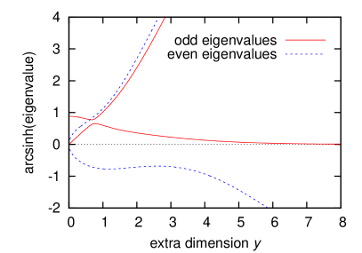
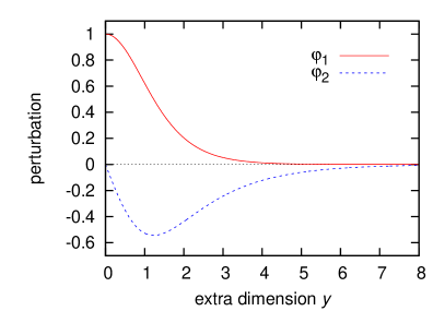
Figure 1: Eigenvalues of the zero-mode solution matrices $M_{E,O}(y)$ (left) and the normalisable zero mode of translation (right) for the flat-space kink-lump $V$-model. The single odd eigenvalue that asymptotes to zero at large $y$ signals the existence of the translation zero mode. Since the other three eigenvalues diverge, there are no other normalisable zero modes.

This plot gives a quantitative summary of the stability behaviour of the background configuration of the $V$-model. According to conjecture one, the existence of an odd eigenvalue $\lambda^{O}$ with $\lambda^{O}\to 0$ as $y\to\infty$, as is apparent in the plot, implies the existence of a normalisable zero mode. The eigenvector corresponding to $\lambda^{O}$ evaluated at large $y$ gives the linear combination of formal zero mode solutions which yield the normalisable zero mode. The resulting initial conditions for this normalisable mode are $(\varphi_{1}(0),\varphi_{2}(0))=(1,0)$ and $(\varphi_{1}^{\prime}(0),\varphi_{2}^{\prime}(0))=(0,-0.77912)$, and the mode is plotted on the right in Figure 1. This mode is exactly the translation zero mode given by equation (7), as expected. The fact that the other three eigenvalues diverge at large $y$ implies, by conjecture one, that there are no more normalisable zero modes for this particular background configuration. By conjecture two, since none of the eigenvalues cross zero there are no negative mass modes, which is again as expected due to our choice of parameters.

Let us now consider the flat $W$-model, which admits similar kink-lump configurations as the $V$-model, but has different behaviour when it comes to the zero modes. The $W$-model has a potential described by equation (9) with superpotential given by

$$W=a\,\Phi_{1}-b\,\Phi_{1}^{3}-c\,\Phi_{1}\Phi_{2}^{2}\>.$$ (48)

This model always has the analytic kink-lump background solution given by equation (47), with the constants in the solution given in terms of the parameters in $W$ as $v^{2}=a/3b$, $k^{2}=4ac^{2}/3b$ and $A^{2}=a/c-2a/3b$. For the following analysis we choose parameters to give the same $v$, $k$ and $A$ as in the $V$-model, namely $a=1.14017$, $b=0.38006$ and $c=0.35834$. The outcome of our analysis is not so dependent on parameter choice since we simply want to demonstrating the existence of zero modes.

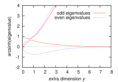
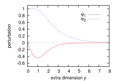
Figure 2: Eigenvalues of the solution matrices (left) and the normalisable even zero mode (right) for the flat-space $W$-model. There are two normalisable zero modes for this model, the other one is the odd translation mode and is exactly the same as in the $V$-model.

As before, we compute the solution matrices and their eigenvalues, the latter of which are shown on the left in Figure 2. From this plot we see that the $W$-model has two normalisable zero modes, one odd and one even, and no negative modes. The normalisable odd mode is the translation mode, and is the same as in the $V$-model. The normalisable even mode has initial conditions $(\varphi_{1}(0),\varphi_{2}(0))=(0,1)$ and $(\varphi_{1}^{\prime}(0),\varphi_{2}^{\prime}(0))=(-0.77912,0)$, and is shown on the right in Figure 2. Physically, this even mode expands both $y$ and $\phi_{2}$, or shrinks both. Although any linear combination of the odd and even normalisable zero modes is again a normalisable zero mode, what is important is that there are a total of two massless physical degrees of freedom. The choice between an odd and even basis, or some other basis without parity, will depend on the physical problem at hand.

Note that in Aybat and George (2010) it is shown that for models generated by a superpotential $W$, exciting the zero modes corresponds to changing the integration constants in the first order equations of motion for the background, $\phi_{i}^{\prime}=W_{i}$. In our example here we have two fields, two integration constants, and so two zero modes. The odd mode changes the value $\phi_{1}(0)$ and the even mode changes $\phi_{2}(0)$. These modes are massless because changes in the initial values $\phi_{i}(0)$ do not change the energy density of the configuration.

In summary, even though the $V$-model and $W$-model have the same background configuration, the former admits only one normalisable zero mode, while the latter admits two. Since the $W$-model contains some extra symmetries owing to its supersymmetric nature, it has the extra zero mode. These results are instructive, although not particularly profound in their own right. The reason we have constructed these two models is so we can compare, qualitatively, what happens when gravity is turned on and the extra dimension is warped.

IV.2 Kink-lump model in warped space

We now look at the existence of zero modes for the kink-lump model when gravity is turned on and the infinite extra dimension is warped, as per a smoothed-out version DeWolfe et al. (2000); Csaki et al. (2000) of Randall-Sundrum Randall and Sundrum (1999). We shall analyse both the $V$- and $W$-models.

The action is given by equation (19) with metric ansatz (20). The scalar potential is

$$V_{\text{warp}}=V+\Lambda\>,$$ (49)

where $V$ is the flat space potential, equation (46), and $\Lambda$ is the bulk cosmological constant required to fine-tune flat 4D slices in the warped space. For stable solutions, constraints on the parameters in the potential are the same as for the flat space case. We can again obtain analytic background solutions, but the relations are now different, being

$$\lambda =2c-4l\>,$$ (50a)

$$\mu_{\chi}^{2} =\frac{lv^{2}}{1+2\kappa^{2}v^{2}}+\frac{\lambda v^{2}(3+8\kappa^{2}v^{2})}{4+8\kappa^{2}v^{2}}\>,$$ (50b)

$$\Lambda =-2\kappa^{2}v^{4}k^{2}\>,$$ (50c)

where $k^{2}=(cv^{2}-\mu_{\chi}^{2})/(1+4\kappa^{2}v^{2})$. Recall that $\kappa$ is the 5D Newton’s constant. With these relations the background configuration is

$$\sigma=\kappa^{2}v^{2}\log\left[\cosh(ky)\right]\>,\qquad\phi_{1}=v\tanh(ky)\>,\qquad\phi_{2}=v\cosh^{-1}(ky)\>.$$ (51)

A representative choice of parameters is $\kappa=1.0$, $l=0.7$, $v=1.0$ and $c=1.5$, with derived parameters $\lambda=0.2$, $\mu_{\chi}^{2}=0.41667$. Plots of the background fields are given in Figure 3. In the gravity-free limit $\kappa\to 0$, and we have $\sigma\to 0$ while $\phi_{1,2}$ retain their kink-lump structure, so we obtain similar solutions as in the flat space case. But we must make it clear that the point in parameter space we have chosen for the warped case is not the same (but it is close to) the point in parameter space that we analysed in the flat case. Nevertheless, since we are interested only in qualitative features of the set-ups, we can still make a fair comparison between the flat and warped configurations.

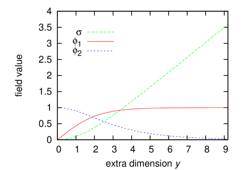
Figure 3: Background configuration for the kink-lump model with a warped extra dimension.

Given this warped background we can proceed to compute the zero mode solution matrices $M_{E,O}(y)$. The metric perturbation $\chi$ (and its counterpart $F$) can be written in terms of the $\psi_{i}$ (counterparts $\varphi_{i}$), so we only need the latter to construct the solution matrices. Now, if we use $\psi_{i}$ to construct the matrices and look for eigenvalues that tend to zero for large $y$, we will obtain modes that are normalisable with respect to the integral $\int\psi^{2}dy$. But what we really want are modes that are normalisable as per equation (26). So in fact we should construct solution matrices from $\varphi_{i}$, which, by equation (22b), is simply $e^{2\sigma}M_{E,O}(y)$, where $M_{E,O}$ here is constructed from $\psi_{i}$.

Figure 4 shows the eigenvalues of the solutions for the warped $V$-model. All of the eigenvalues diverge for large $y$ so there are no zero modes in the physical spectrum. In particular, the translation zero mode does not survive in the presence of gravity, in concordance with the results of Shaposhnikov et al. (2005). Similarly, since none of the eigenvalues pass through zero, there are no negative modes in the spectrum either. This is also as expected since we restricted our parameters so the configuration would be stable. In summary, the $V$-model in warped space has no normalisable negative modes and no normalisable zero modes.

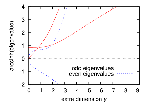
Figure 4: Eigenvalues for odd and even zero modes for the $V$-model with a warped extra dimension. All eigenvalues diverge for large $y$ so there are no normalisable zero modes. Since the eigenvalues do not pass through zero, so there are also no negative modes.

Now consider the $W$-model in warped space. We use the same superpotential as given by equation (48), but now the derived potential $V$ is modified, as per equation (36). Such a potential is again, as in the flat space case, qualitatively similar to the $V$-model. In fact, for the choice of parameters $b=c$, we can get analytic solutions of exactly the same form as the warped $V$-model, equation (51) (such a model is used in Bazeia and Gomes (2004)). The parameters of this solution in terms of the parameters in $W$ are $v^{2}=a/3b$ and $k^{2}=4ab/3$. To obtain a background with exactly the same form as the one we used in the analysis of the $V$-model we choose $a=0.69821$ and $b=c=0.23274$; the background is show in Figure 3. The conclusions that we shall draw regarding zero modes are generically the same for a large parameter range, but we make this choice so we can compare with the $V$-model.

The eigenvalues of the solution matrix for the physical perturbations $\varphi_{i}$ for the warped $W$-model are shown on the left in Figure 5. As can be seen, there is a surviving even zero mode. The initial conditions for this mode are $(\varphi_{1}(0),\varphi_{2}(0))=(0,1)$ and $(\varphi_{1}^{\prime}(0),\varphi_{2}^{\prime}(0))=(-0.172148,0)$ and the mode is plotted on the right in Figure 5. It is normalisable, as per equation (26), and the surface terms, equation (28), vanish at large $y$. The mode is therefore present in the physical spectrum. It has a qualitatively similar form to the even zero mode in the flat $W$-model. Finally, no eigenvalue crosses zero, so there are no negative modes in the spectrum, a result which is already known for general $W$ Aybat and George (2010).

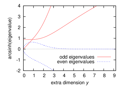
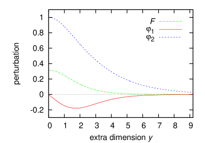
Figure 5: Eigenvalues of the solution matrix (left) and the single normalisable zero mode (right) for the warped-space $W$-model. Compare with the flat-space $W$-model, Figure 2, which has two zero modes, and the warped-space $V$-model, Figure 4, which has no zero modes.

Even though the potentials of the four models we have looked at (flat and warped, $V$- and $W$-models) are qualitatively very similar and admit the same background configurations, they show very different behaviour when it comes to having zero modes in the physical spectrum. Our general conclusion is that adding gravity in the form of a warped extra dimension will remove the translation zero mode from the spectrum, but will not necessarily remove other zero modes. In this section we have also explicitly shown how the eigenvalues of the solution matrices $M_{E,O}(y)$ allow one to easily find normalisable zero modes. Furthermore, our analysis of the warped $V$-model shows, at least for some values of the parameters, that it contains no zero modes. It is therefore phenomenologically acceptable to use this type of set-up for constructing realistic models, as is done in Davies et al. (2008).

V Domain-wall soft-wall models

In this section we briefly analyse another example model, one with a compact extra dimension and $N=2$ scalars. The potential is generated by a superpotential with gravity and we show that a zero mode again survives in this compact set-up. The model was first presented in Aybat and George (2010) as a realisation of a domain-wall soft-wall model, where the extra dimension is dynamically compactified by the formation of curvature singularities.

The superpotential is

$$W=\alpha\sinh(\nu\,\Phi_{1})+(a\,\Phi_{2}-b\,\Phi_{2}^{3})\>.$$ (52)

For background configurations of definite parity with both scalars odd there is a unique solution to the first order equations of motion:

$$\sigma =\frac{-\kappa^{2}}{\nu^{2}}\log\left[\cos\left(\alpha\nu^{2}y\right)\right]+\frac{\kappa^{2}a}{18b}\left\{1+4\log\left[\cosh\left(\sqrt{3ab}\,y\right)\right]-\cosh^{-2}\left(\sqrt{3ab}\,y\right)\right\}\>,$$ (53a)

$$\phi_{1} =\frac{2}{\nu}\operatorname{arctanh}\left[\tan\left(\frac{\alpha\nu^{2}y}{2}\right)\right]\>,$$ (53b)

$$\phi_{2} =\sqrt{\frac{a}{3b}}\tanh\left(\sqrt{3ab}\,y\right)\>.$$ (53c)

The edge of extra dimension is fixed at $y_{*}=\pi/2\alpha\nu^{2}$. We choose parameters $\alpha=1.0$, $\nu=1.4$, $a=0.5$ and $b=0.3$ and plot the background in Figure 6. In Aybat and George (2010) it was shown that enforcing odd parity on the fields $\Phi_{1,2}$ themselves, as opposed to just the background configuration, ensures that there are no normalisable zero modes in the spectrum. We shall now show that relaxing the parity condition leads to the appearance of a zero mode that de-stabilises the background.

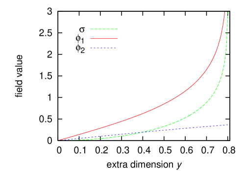
Figure 6: Domain-wall soft-wall background configuration. $\phi_{1}$ acts like a dilaton, while $\phi_{2}$ takes on a (very wide) domain-wall solution. The extra dimension ends at a physical curvature singularity at $y_{*}=0.80143$.

For the background configuration and choice of parameters given above we compute the solution matrices $M_{E,O}(y)$ for the physical perturbations $\varphi_{i}$. The eigenvalues of these two matrices are show on the left in Figure 7. Three of the eigenvalues diverge as $y\to y_{*}$, but the other one remains finite. Even though our first conjecture states that we must look for eigenvalues that tend to zero to find normalisable modes, we find that this finite eigenvalue does actually correspond to a properly normalisable mode. Since our space is finite, if $\varphi_{i}$ and $F$ remain finite throughout the extra dimension they will be physically allowed perturbations (a small multiple of them will be small compared with $\phi_{i}$ and $\sigma$). The initial conditions for the normalisable mode corresponding to the finite odd eigenvalue are $(\varphi_{1}(0),\varphi_{2}(0))=(-0.19847,1)$ and $(\varphi_{1}^{\prime}(0),\varphi_{2}^{\prime}(0))=(0,0)$. This mode is shown on the right in Figure 7. It is normalisable as per equation (26), and the relevant surface terms in the effective 4D action vanish because $e^{-4\sigma}\to 0$ at the boundaries of the extra dimension. This zero mode has opposite parity to the background, so if one does not enforce parity on the fields themselves this mode will exist in the 4D spectrum and the background configuration will not be stable.

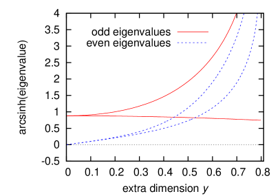
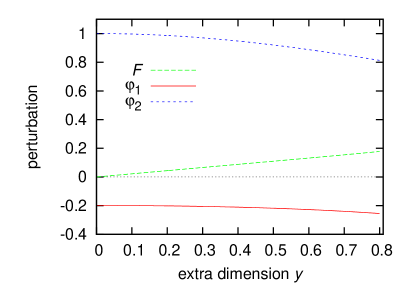
Figure 7: Eigenvalues of the solution matrices (left) and the normalisable odd zero mode (right) for the domain-wall soft-wall model.

As we have shown, the eigenvalues of the solution matrices are also useful for finding zero modes when the extra dimension is compact and the perturbations are allowed to be finite over all $y$. The domain-wall soft-wall model in Aybat and George (2010) contains a normalisable zero mode which must be removed by enforcing parity on the fields themselves (the model-building philosophy of these set-ups forbids adding fundamental branes to restrict the boundary conditions of the KK modes, thereby eliminating any zero modes). Alternatively, we suggest that it may be possible to construct a domain-wall soft-wall model using a normal potential $V$ that does not have the extra symmetries inherent in the superpotential approach, and hence does not have a surviving zero mode.

VI Conclusions

In this paper we looked at scalar perturbations around a background configuration, and were concerned with finding zero modes. Both flat and warped extra dimensions were studied, with both a general scalar potential $V$, and a potential generated by a superpotential $W$. The results can be split into three main parts: analytic zero mode solutions, use of these solutions, and examples. In Section II we presented analytic expressions for formal zero mode solutions to the perturbation equations, with particular emphasis on the $N=2$ scalar case. For $N=2$ scalars in warped space with a potential generated by a superpotential we found analytic closed-form expressions for the four, linearly independent zero modes solutions. Section III discusses the use of formal zero modes, and here we made two conjectures which use the eigenvalues of the solution matrices: one states how to find normalisable zero modes, the other tells how many normalisable negative modes there are in the spectrum. In Sections IV and V we looked at some specific example models to demonstrate the workings of these conjectures, and to show that normalisable zero modes can survive when the extra dimension is warped.

Our general conclusions regarding extra-dimensional model building are the following. If one uses a general potential $V$ then in flat space there will exist the translation zero mode, which is removed from the 4D KK spectrum when the extra dimension is warped (for $N=1$ scalar this conclusion was made in Shaposhnikov et al. (2005)). But it is not always the case that all spin-0 zero modes are removed by the inclusion of gravity. We have shown that models which have $N=2$ scalars and generate the potential from a superpotential generally admit an extra zero mode which survives in the presence of gravity. Such superpotential models are widely studied in the literature for the reason that they give first-order equations of motion. But without some extra input, like a fundamental brane or forced parity, these superpotential models will be phenomenologically unacceptable due to the presence of massless spin-0 degrees of freedom, something which we have not observed in nature.

Finally, the general solutions we have found for the fake supergravity scenario with $N=2$ scalars rely only on the metric ansatz (20) and should have wider applicability than to the domain-wall models that we emphasise here. For example, the inclusion of fundamental brane terms would change only the boundary conditions; the bulk solutions we have found will remain the same. Extending the zero mode solutions to more than one extra dimension may also be possible, following the analysis of Underwood (2011).

Appendix A Reduction of order of a set of linear homogeneous ordinary differential equations

Any set of linear homogeneous ODEs which is $n^{\text{th}}$ order can be easily recast as a set of $n$ first order differential equations. We assume this has been done and that the resulting $n$ dependent variables $f_{i}(y)$, where $i=1\ldots n$ and $y$ is the independent variable, satisfy the equations

$$f_{i}^{\prime}(y)=A_{ij}(y)f_{j}(y)\>.$$ (54)

There is an implicit sum over $j$. This equation has $n$ independent solutions. If we know $m$ of these solutions then we can perform reduction of order on (54) to obtain a set of $n-m$ coupled first order ODEs. We outline this procedure, which follows closely that given in Coddington and Levinson (1955).

Write equation (54) as a matrix equation, $f^{\prime}(y)=A(y)\cdot f(y)$, where $f(y)$ is a vector of length $n$ made of the dependent variables. Let $F_{s}$ be the $n\times n$ solution matrix of this ODE, such that each column of $F_{s}$ is an independent solution vector $f^{(s)}(y)$. It must be that $\det F_{s}\neq 0$ for all $y$. Then $F_{s}$ is known as the fundamental matrix of the set of ODEs specified by $A$, since $F_{s}$ determines $A$ uniquely by $A=F_{s}^{\prime}F_{s}^{-1}$ (the converse is not true since $F_{s}\cdot(\text{const matrix})$ is also a fundamental matrix of $A$).

Reduction of order then proceeds as follows. Assume we know $m$ columns of $F_{s}$ (that is, $m$ linearly independent solutions of the ODE) which we label $f^{(s_{i})}$ with $i=1\ldots m$. Then construct the $n\times n$ matrix

$$U=\left(f^{(s_{1})},\,f^{(s_{2})},\,\ldots,\,f^{(s_{m})},\,a^{(m+1)},\,\ldots,\,a^{(n)}\right)\>,$$ (55)

where the $a^{(j)}$, $j=m+1\ldots n$, are linearly independent constant vectors. They can be freely chosen, so long as $\det U\neq 0$ for all $y$. Usually the $a^{(j)}$ can be unit vectors. Now change variables to $g$ by the definition $f=U\cdot g$ and the equation $f^{\prime}=A\cdot f$ becomes

$$g^{\prime}=U^{-1}\cdot A\cdot\left(0,\,\ldots,\,0,\,a^{(m+1)},\,\ldots,\,a^{(n)}\right)\cdot g\>.$$ (56)

The first $m$ components of the vector $g$ do not appear on the right-hand-side of this ODE (after multiplying the matrices out), so this procedure decouples $m$ of the equations. Call the solutions to equation (56) $g^{(s_{i})}$. We know $m$ of these are just constant vectors: $g^{(s_{1})}=(1,\,0,\,\ldots,\,0)$, $g^{(s_{2})}=(0,\,1,\,0,\,\ldots,\,0)$ and so on to $g^{(s_{m})}$. The remaining $n-m$ solutions are to be determined using other techniques. Once they are found, the remaining solutions to the original ODE are given by $f^{(s_{j})}=U\cdot g^{(s_{j})}$.

References

- Rubakov and Shaposhnikov (1983) V. A. Rubakov and M. E. Shaposhnikov, Phys. Lett. B125, 136 (1983).
- Goldberger and Wise (1999) W. D. Goldberger and M. B. Wise, Phys. Rev. Lett. 83, 4922 (1999), eprint hep-ph/9907447.
- Csaki et al. (2001) C. Csaki, M. L. Graesser, and G. D. Kribs, Phys. Rev. D63, 065002 (2001), eprint hep-th/0008151.
- Randall and Sundrum (1999) L. Randall and R. Sundrum, Phys. Rev. Lett. 83, 4690 (1999), eprint hep-th/9906064.
- Csaki et al. (2000) C. Csaki, J. Erlich, T. J. Hollowood, and Y. Shirman, Nucl. Phys. B581, 309 (2000), eprint hep-th/0001033.
- Gremm (2000) M. Gremm, Phys.Rev. D62, 044017 (2000), eprint hep-th/0002040.
- Karch et al. (2006) A. Karch, E. Katz, D. T. Son, and M. A. Stephanov, Phys. Rev. D74, 015005 (2006), eprint hep-ph/0602229.
- Davies et al. (2008) R. Davies, D. P. George, and R. R. Volkas, Phys. Rev. D77, 124038 (2008), eprint 0705.1584.
- Aybat and George (2010) S. M. Aybat and D. P. George, JHEP 09, 010 (2010), eprint 1006.2827.
- Toharia and Trodden (2008a) M. Toharia and M. Trodden, Phys.Rev.Lett. 100, 041602 (2008a), eprint 0708.4005.
- Toharia and Trodden (2008b) M. Toharia and M. Trodden, Phys.Rev. D77, 025029 (2008b), eprint 0708.4008.
- Kobayashi et al. (2002) S. Kobayashi, K. Koyama, and J. Soda, Phys.Rev. D65, 064014 (2002), eprint hep-th/0107025.
- Toharia (2008) M. Toharia (2008), eprint 0803.2503.
- Toharia et al. (2010) M. Toharia, M. Trodden, and E. J. West, Phys.Rev. D82, 025009 (2010), eprint 1002.0011.
- Underwood (2011) B. Underwood, Class.Quant.Grav. 28, 195013 (2011), eprint 1009.4200.
- Berg et al. (2006) M. Berg, M. Haack, and W. Mueck, Nucl.Phys. B736, 82 (2006), eprint hep-th/0507285.
- Berg et al. (2008) M. Berg, M. Haack, and W. Mueck, Nucl.Phys. B789, 1 (2008), eprint hep-th/0612224.
- Elander (2010) D. Elander, JHEP 1003, 114 (2010), eprint 0912.1600.
- Elander and Piai (2011) D. Elander and M. Piai, JHEP 1101, 026 (2011), eprint 1010.1964.
- Shaposhnikov et al. (2005) M. Shaposhnikov, P. Tinyakov, and K. Zuleta, JHEP 09, 062 (2005), eprint hep-th/0508102.
- Bazeia et al. (2010) D. Bazeia, M. M. Ferreira, Jr., A. R. Gomes, and R. Menezes, Physica D239, 942 (2010), eprint 1001.5286.
- DeWolfe et al. (2000) O. DeWolfe, D. Z. Freedman, S. S. Gubser, and A. Karch, Phys. Rev. D62, 046008 (2000), eprint hep-th/9909134.
- Freedman et al. (2004) D. Z. Freedman, C. Nunez, M. Schnabl, and K. Skenderis, Phys. Rev. D69, 104027 (2004), eprint hep-th/0312055.
- Amann and Quittner (1995) H. Amann and P. Quittner, J. Math. Phys. 36, 4553 (1995).
- Garaud and Volkov (2010) J. Garaud and M. S. Volkov, Nucl.Phys. B839, 310 (2010), eprint 1005.3002.
- Davies (2007) R. Davies, Master’s thesis, University of Melbourne (2007).
- Bazeia and Gomes (2004) D. Bazeia and A. R. Gomes, JHEP 05, 012 (2004), eprint hep-th/0403141.
- Elander et al. (2010) D. Elander, C. Nunez, and M. Piai, Phys.Lett. B686, 64 (2010), eprint 0908.2808.
- Coddington and Levinson (1955) E. A. Coddington and N. Levinson, Theory of ordinary differential equations (McGraw-Hill, New York, 1955).