MOA-2009-BLG-387Lb: A massive planet orbiting an M dwarf

Abstract

Aims. We report the discovery of a planet with a high planet-to-star mass ratio in the microlensing event MOA-2009-BLG-387, which exhibited pronounced deviations over a 12-day interval, one of the longest for any planetary event. The host is an M dwarf, with a mass in the range $0.07\,M_{\odot}<M_{\rm host}<0.49\,M_{\odot}$ at 90% confidence. The planet-star mass ratio $q=0.0132\pm 0.003$ has been measured extremely well, so at the best-estimated host mass, the planet mass is $m_{p}=2.6$ Jupiter masses for the median host mass, $M=0.19\,M_{\odot}$.

Methods. The host mass is determined from two “higher order” microlensing parameters. One of these, the angular Einstein radius $\theta_{\rm E}=0.31\pm 0.03\,$mas has been accurately measured, but the other (the microlens parallax $\pi_{\rm E}$, which is due to the Earth’s orbital motion) is highly degenerate with the orbital motion of the planet. We statistically resolve the degeneracy between Earth and planet orbital effects by imposing priors from a Galactic model that specifies the positions and velocities of lenses and sources and a Kepler model of orbits.

Results. The 90% confidence intervals for the distance, semi-major axis, and period of the planet are $3.5\,{\rm kpc}<D_{L}<7.9\,{\rm kpc}$, $1.1\,{\rm AU}<a<2.7\,{\rm AU}$, and $3.8\,{\rm yr}<P<7.6\,{\rm yr}$, respectively.

1 Introduction

Over the past decade, the gravitational microlensing method has led to detection of ten exoplanets (Bond et al. 2004; Udalski et al. 2005; Beaulieu et al. 2006; Gould et al. 2006; Gaudi et al. 2008; Bennett et al. 2008; Dong et al. 2009b; Janczak et al. 2010; Sumi et al. 2010), which permits the exploration of host-star and planet populations whose mass and distance are not probed by any other method. Indeed, since the efficiency of the microlensing method does not depend on detecting light from the host star, it allows one to probe essentially all stellar types over distant regions of our Galaxy. In particular, microlensing is an excellent method to explore planets around M dwarfs, which are the most common stars in our Galaxy, but which are often a challenge for other techniques because of their low luminosity. Roughly half of all microlensing events toward the Galactic bulge stem from stars with mass $\la 0.5\leavevmode\nobreak\ M_{\odot}$ (Gould 2000).

Determining the characteristics and frequency of planets orbiting M dwarfs is of interest not only because M dwarfs are the most common type of stars in the Galaxy, but also because these systems provide important tests of planet formation theories. In particular, the core accretion theory of giant planet formation predicts that giant planets should be less common around low-mass stars (Laughlin et al. 2004; Ida & Lin 2005; Kennedy & Kenyon 2008; D’Angelo et al. 2010), whereas the gravitational instability model predicts that giant planets can form around M dwarfs with sufficiently massive protoplanetary disks (Boss 2006). In fact, there is accumulating evidence from radial velocity surveys that giant planets are less common around low-mass primaries (Cumming et al. 2008; Johnson et al. 2010). However, these surveys are only sensitive to planets with semimajor axes of $<2.5\leavevmode\nobreak\ {\rm AU}$. Since it is thought that the majority of the giant planets found by radial velocity surveys likely formed farther out in their protoplanetary disks and subsequently migrated close to their parent star, it is not clear whether the relative paucity of giant planets around low-mass stars found in these surveys is a statement about the dependence on stellar mass of migration or of formation.

Microlensing is complementary to the radial velocity technique in that it is sensitive to planets with larger semimajor axes, closer to their supposed birth sites. Indeed, based on the analysis of 13 well-monitored high-magnification events with 6 detected planets, Gould et al. (2010) found that the frequency of giant planets at separations of $\sim 2.5\leavevmode\nobreak\ {\rm AU}$ orbiting $\sim 0.5\leavevmode\nobreak\ M_{\odot}$ hosts was quite high and, in particular, consistent with the extrapolation of the frequencies of small-separation giant planets orbiting solar mass hosts inferred from radial velocity surveys out to the separations where microlensing is most sensitive. This suggests that low-mass stars may form giant planets as efficiently as do higher mass stars, but that these planets do not migrate as efficiently.

Furthermore, of the ten previously published microlensing planets, one was a “supermassive” planet with a very high mass ratio: a $m_{p}=3.8M_{\rm Jup}$ planet orbiting an M dwarf of mass $M=0.46\leavevmode\nobreak\ M_{\odot}$ (Dong et al. 2009a). Given their high planet-to-star mass ratios $q$, such planets are expected to be exceedingly rare in the core-accretion paradigm, so the mere existence of this planet may pose a challenge to such theories. Gravitational instability, on the other hand, favors the formation of massive planets (provided they form at all).

Current and future microlensing surveys are particularly sensitive to large $q$ planets orbiting M dwarf hosts, for several reasons. As with other techniques, microlensing is more sensitive to planets with higher $q$. In addition, as the mass ratio increases, a larger fraction of systems induce an important subclass of resonant-caustic lenses. Resonant caustics are created when the planet happens to have a projected separation close to the Einstein radius of the primary (Wambsganss 1997). The range of separations that give rise to resonant caustics is quite narrow for small $q$, but grows as $q^{1/3}$. Furthermore, although the range of parameter space giving rise to resonant caustics is narrow, the caustics themselves and their cross sections are large and also grow as $q^{1/3}$. Thus the probability of detecting planets via these caustics is relatively high, and such systems contribute a significant fraction of all detected events, particularly for supermassive planets orbiting M dwarfs. Events due to resonant caustics are particularly valuable, as they allow one to further constrain the properties and orbit of the planet. This is because these events usually exhibit caustic features that are separated well in time. When combined with the fact that the precise shape of a resonant caustic is extremely sensitive to the separation of the planet from the Einstein ring, such light curves are particularly sensitive to orbital motion of the planet (see, e.g., Bennett et al. 2010).

Here we present the analysis of the microlensing event MOA-2009-BLG-387, a resonant-caustic event, which we demonstrate is caused by a massive planet orbiting an M dwarf. The light curve associated with this event contains very prominent caustic features that are well separated in time. These structures were very intensively monitored by the microlensing observers, so that the geometry of the system is quite well constrained. As a result, the event has high sensitivity to two higher order effects: parallax and orbital motion of the planet. In Section 4, we present the modeling of these two effects and our estimates of the event characteristics. This analysis reveals a degeneracy between one component of the parallax and one component of the orbital motion. We explain, for the first time, the causes of this degeneracy. It gives rise to very large errors in both the parallax and orbital motion, which makes the final results highly sensitive to the adopted priors. In particular, uniform priors in microlensing variables imply essentially uniform priors in lens-source relative parallax, whereas the proper prior for physical location is uniformity in volume element. These differ by approximately a factor $D_{l}^{4}$, where $D_{l}$ is the lens distance. In Section 5, we therefore give a careful Bayesian analysis that properly weights the distribution by correct physical priors. The high-mass end of the range still permitted is eliminated by the failure to detect flux from the lens using high-resolution NACO images on the VLT. Combining all available information, we find that the host is an M dwarf in the mass range $0.07\,M_{\odot}<M_{\rm host}<0.49\,M_{\odot}$ at 90% confidence.

2 Observational data

The microlensing event MOA-2009-BLG-387 was alerted by the MOA collaboration (Microlensing Observations in Astrophysics) on 24 July 2009 at 15:08 UT, $HJD^{\prime}\equiv HJD-2,450,000=5037.13$, a few days before the first caustic entry. Many observatories obtained data of the event. The celestial coordinates of the event are $\alpha=17h53m50.79s$ and $\delta=-33^{\circ}59^{\prime}25^{\prime\prime}$ (J2000.0) corresponding to Galactic coordinates : $l=+356.56$, $b=-4.097$.

The lightcurve is overall characterized by two pairs of caustic crossings (entrance plus exit), which together span 12 days (see Figure1). This structure is caused by the source passing over two “prongs” of a resonant caustic (see Figure1 inset). Obtaining good coverage of these caustic crossings posed a variety of challenges.

The first caustic entrance ($HJD^{\prime}=5040.3$) was detected by the PLANET collaboration using the South African Astronomical Observatory (SAAO) at Sutherland (Elizabeth 1m) who then issued an anomaly alert at $HJD^{\prime}$ 5040.4 calling for intensive follow-up observations, which in turn enabled excellent coverage of the first caustic exit roughly one day later.

The second caustic entrance occurred about seven days later ($HJD^{\prime}=5047.1$, see Figure1). That the caustic crossings are so far apart in time is quite unusual in planetary microlensing events. Since round-the-clock intensive observations cannot normally be sustained for a week, accurate real-time prediction of the second caustic entrance was important for obtaining intensive coverage of this feature. In fact, the second caustic entrance was predicted 14 hours in advance, with a five-hour discrete uncertainty due to the well-known close/wide $s\leftrightarrow s^{-1}$ degeneracy, where $s$ is the projected separation in units of the Einstein radius. The close-geometry crossing prediction was accurate to less than one half hour and the caustic-geometry prediction was almost identical to the one derived from the best fit to the full lightcurve, which is shown in Figure1.

The extended duration of the lightcurve anomalies indicates a correspondingly large caustic structure. Indeed, the preliminary models found a planet/star separation (in units of Einstein radius) close to unity, which means that the caustic is resonant (see the caustic shape in the upper panel of Figure1, where the source is going upward).

The event was alerted and monitored by the MOA collaboration. It was also monitored by the Probing Lensing Anomalies Network collaboration (PLANET; Albrow et al. 1998) from three different telescopes: at the South African Astronomical Observatory (SAAO), as mentioned above, as well as the Canopus 1 m at Hobart (Tasmania) and the 60 cm of Perth Observatory (Australia).

The Microlensing Follow Up Network ($\mu$FUN ; Yoo et al. 2004) followed the event from Chile (1.3m SMARTS telescope at CTIO) (V, I and H band data), South Africa (0.35 m telescope at Bronberg observatory), New Zealand (0.40 m and 0.35 m telescopes at Auckland Observatory (AO) and Farm Cove (FCO) observatory, respectively, the Wise observatory (1.0 m at Mitzpe Ramon, Israel), and the Kumeu observatory (0.36 m telescope at Auckland, NZ).

The RoboNet collaboration also followed the event with their three 2m robotic telescopes : the Faulkes Telescopes North (FTN) and South (FTS) in Hawaii and Australia (Siding Springs Observatory) respectively, and the Liverpool Telescope (LT) on La Palma (Canary Islands). And finally, the MiNDSTEp collaboration observed the event with the Danish 1.54 m at ESO La Silla (Chile).

Observational conditions for this event were unusually challenging, due in part to the faintness of the target and the presence of a bright neighboring star. Moreover, the full moon passed close to the source near the second caustic entrance. As a result, several data sets were of much lower statistical quality and had much stronger systematics than the others. We therefore selected seven data sets that cover the caustic features and the entire lightcurve : MOA, SAAO, FCO, AO, Danish, Bronberg, and Wise. They include 118 MOA data points in I band, 221 PLANET data points in I band, 262 $\mu$FUN data points in unfiltered, R and I bands, and 300 MiNDSTEp data points in I band. We also fit the $\mu$FUN CTIO I and V data to the final model, but solely for the purpose of determining the source size. And finally, we fit $\mu$FUN CTIO $H$-band data to the lightcurve in order to compare the $H$-band source flux with the late-time $H$-band baseline flux from VLT images (see Section 2.1). The SAAO, FCO, AO, Danish, Bronberg, and Wise data were reduced by MDA using the PYSIS3 software (Albrow et al. 2009). The FCO, AO, Bronberg, and Wise images were taken in white light and suffered from systematic effects related to the airmass. Such effects were corrected by extracting lightcurves of other stars in the field with similar colors to the lens, and assuming that these stars are intrinsically constant.

For each data set, the errors were rescaled to make $\chi^{2}$ per degree of freedom for the best binary-lens fit close to unity. We then eliminated the largest outlier and repeated the process until there were no 3 $\sigma$ outliers.

2.1 VLT NACO Images

On 7 June 2010, we obtained high-resolution $H$-band images using the NACO imager on the Very Large Telescope (VLT). Since this was approximately 7.7 Einstein timescales after the peak of the event, the source was essentially at the baseline. The reduction procedures were similar to those of MOA-2008-BLG-310, which are described in detail by Janczak et al. (2010).

To identify the source on the NACO frame, we first performed image subtraction on CTIO $I$-band images to locate its position on the $I$-band frame. We then used the NACO image to find relatively unblended stars that could be used to align the $I$-band and NACO frames. There is clearly a source at the inferred position, but it lies only seven pixels ($0.19^{\prime\prime}$) from an ambient star, which is 1.35 mag brighter than the “target” (source plus lens plus any other blended light within the aperture). This proximity induces a 94% correlation coefficient between the photometric measurements of the two stars. We therefore estimate the target error as 0.06 mag. In the NACO system (which is calibrated to 2MASS using comparison stars) the target magnitude is

$$H_{\rm target,NACO}=18.25\pm 0.06.$$ (1)

We have an $H$-band light curve (taken simultaneously with $V$ and $I$ at CTIO), and so (once we have established a model fit the light curve in Section 4) we can measure quite precisely the source flux in the CTIO system, $H_{\rm source,CTIO}=20.03\pm 0.02$. To compare with NACO, we transform to the NACO system using 4 comparison stars that are relatively unblended, a process to which we assign a 0.03 mag error, finding

$$H_{\rm source,NACO}=18.35\pm 0.03.$$ (2)

The difference, consisting of light from the lens as well as any other blended light in the aperture, is $0.10\pm 0.07$.

This excess-flux measurement could in principle be due to five physical effects. First, it is reasonably consistent with normal statistical noise. Second, it could come from the lens. As we show in Section 5, this would be consistent with a broad range of M dwarf lenses. Third, it could be a companion to the source, and fourth, a companion to the lens. Finally, it could be an ambient star unrelated to the event. The fundamental importance of this measurement is that, for all five of these possibilities, the measurement places an upper limit on the flux from the lens, hence its mass (assuming it is not a white dwarf).

3 Source properties from color-magnitude diagram and measurement of $\theta_{\rm E}$

To determine the dereddened color and magnitude of the microlensed source, we put the best fit color and magnitude of the source on an $(I,V-I)$ instrumental color magnitude diagram (CMD) (cf. Fig.2), using instrumental CTIO data. The magnitude and color of the target are $I=20.62\pm 0.04$ and $(V-I)=-0.42\pm 0.01$. The mean position of the red clump is represented by an open circle at $(I,V-I)_{RC}=(16.36,-0.16)$, with an error of 0.05 for both quantities.

For the absolute clump magnitude, we adopt $M_{I,RC}=-0.25\pm 0.05$ from Bennett et al. (2010). We adopt the measured bulge clump color $(V-I)_{0,RC}=1.08\pm 0.05$ (Fig. 5 of Bensby et al. 2010) and a Galactocentric distance $R_{0}=8.0\pm 0.3\,$kpc (Yelda et al. 2010). We further assume that at the longitude ($l=-3.4$), the bar lies 0.7 kpc more distant than $R_{0}$ (D. Nataf et al., in preparation), i.e., 8.7 kpc. From this, we derive $(I,V-I)_{0,RC}=(14.45,1.08)\pm(0.10,0.05)$, so that the dereddened source color and magnitude are given by: $(I,V-I)_{0}=\Delta(I,V-I)+(I,V-I)_{0,RC}=(18.71,0.82)$. From $(V-I)_{0}$, we derive $(V-K)_{0}=1.78\pm 0.14$ using the Bessel & Brett (1988) color-color relations.

The color determines the relation between dereddened source flux and angular source radius, (Kervella et al. 2004)

$$\log{2\theta_{*}}=0.5170-0.2V_{0}+0.2755(V-K)_{0},$$ (3)

giving $\,\theta_{*}=0.63\pm 0.06\,\mu{\rm as}$. With the angular size of the source given by the limb-darkened extended-source fit (model 5, see Table 1), $\rho_{*}=0.00202\pm 0.00003$, we derive the angular Einstein radius $\theta_{\rm E}$ : $\theta_{\rm E}=\theta_{*}/\rho_{*}=0.31\pm 0.03\,\rm{mas}$.

4 Event modeling

4.1 Overview

The modeling proceeds in several stages. We first give an overview of these stages and then consider them each in detail. First, inspection of the lightcurve shows that the source crossed over two “prongs” of a caustic, or possibly two separate caustics, with a pronounced trough in between. The source spent 1-3 days crossing each prong and 7 days between prongs. This pattern strongly implies that the event topology is that of a source crossing the “back end” of a resonant caustic with $s<1$, as illustrated in Figure1. We nevertheless conducted a blind search of parameter space, incorporating the minimal 6 standard static-binary parameters required to describe all binary events, as well as $\rho=\theta_{*}/\theta_{\rm E}$, the source size in units of the Einstein radius. The parameters derived from this fit are quite robust. However, they yield only the planet-star mass ratio $q$, but not the planet mass $m_{p}=qM$, where $M$ is the host mass. In principle, one can measure $M$ from (e.g. Gould 2000)

$$M=\frac{\theta_{\rm E}}{\kappa\pi_{\rm E}}$$ (4)

where $\pi_{\rm E}$ is the “microlens parallax” and $\kappa\equiv 4G/(c^{2}\,{\rm AU})\sim 8.1\,{\rm mas}\,M_{\odot}^{-1}$. However, while $\theta_{\rm E}=\theta_{*}/\rho$ is also quite robustly determined from the static solution (and Section 3), $\pi_{\rm E}$ is not.

However, the event timescale is moderately long ($\sim 40$ days). This would not normally be long enough to measure the full microlens parallax, but might be enough to measure one dimension of the parallax vector (Gould, Miralda-Escude & Bahcall 1994). Moreover, the large separation in time of the caustic features could permit detection of orbital motion effects as well (Albrow et al. 2000). We therefore incorporate these two effects, first separately and then together. We find that each is separately detected with high significance, but that when combined they are partially degenerate with each other. In particular, one of the two components of the microlensing parallax vector $\@vec{\pi}_{\rm E}$ is highly degenerate with one of the two measurable parameters of orbital motion. It is often the case that one or both components of $\@vec{\pi}_{\rm E}$ are poorly measured in planetary microlensing events. The usual solution is to adopt Bayesian priors for the lens-source relative parallax and proper motion, based on a Galactic model. We also pursue this approach, but in addition we consider separately Bayesian priors on the orbital parameters as well. We show that the results obtained by employing either set of priors separately are consistent with each other, and we therefore combine both sets of priors.

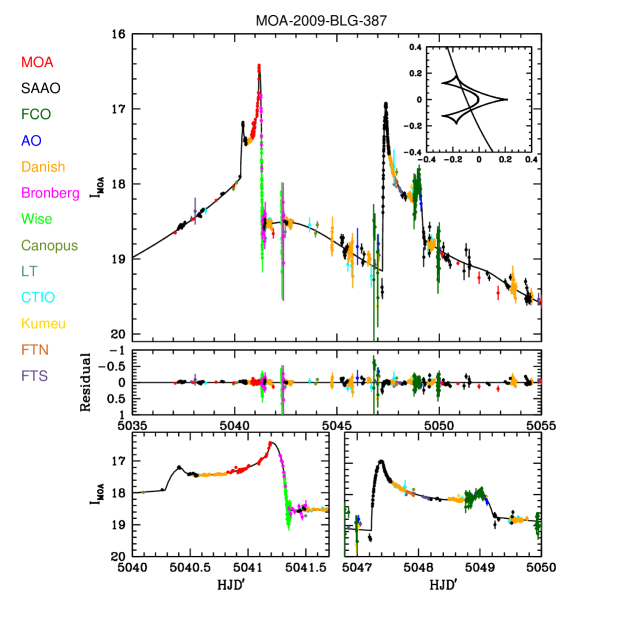
Figure 1: Top: Light curve of MOA-2009-BLG-387 near its peak in July 2009 and the trajectory of the source across the caustic feature on the right. The source is going upward. We show the model with finite-source, parallax and orbital motion effects. Middle: Magnitude residuals. Bottom: Zooms of the caustic features of the light curve.

Figure 2: Instrumental color-magnitude diagram of the field around MOA-2009-BLG-387. The clump centroid is shown by an open circle, while the CTIO $I$ and $V-I$ measurements of the source are shown by a filled circle

4.2 Static binary

A static binary-lens point-source model involves six microlensing parameters: three related to the lens-source kinematics ($t_{0}$, $u_{0}$, $t_{E}$), where $t_{0}$ is the time of lens-source closest approach, $u_{0}$ is the impact parameter with respect to the center of mass of the binary-lens system and $t_{E}$ is the Einstein timescale of the event, and three related to the binary-lens system ($q$, $s$, $\alpha$), where $q$ and $s$ are the planet-star mass ratio and separation in units of Einstein radius, respectively, and $\alpha$ is the angle between the trajectory of the source and the star-planet axis. For $n=7$ observatories, there are $2n$ photometric parameters, $n\times(F_{s},F_{b})$, which correspond to the source flux and blend flux for each data set. These are usually determined by linear regression. The radius of the source, $\rho$, in Einstein units, can also be derived from the model provided that the source passes over, or sufficiently close to, a caustic structure. To optimize the fit in terms of computing time, we adopt different methods for implementing finite-source effects, depending on the distance between the source and the caustic features in the sky plane. When the source is far from the caustic (in the wings of the lightcurve), we treat it as a point source. In the caustic crossing regions, we use a finite-source model based on the Green-Stokes theorem (Gould & Gaucherel 1997). Numerical implementation of this method is adapted from the code that was originally devised for Albrow et al. (2001) and refined in An et al. (2002). This technique, which reduces the 2-dimensional integral over the source to a 1-dimensional integral over its boundary and so is extremely efficient, implicitly assumes that the source has uniform surface brightness, i.e., is not limb darkened. We then include limb-darkening in the final fit, as described in Section 4.6. Lastly, in the intermediary regions, we use the hexadecapole approximation (Pejcha & Heyrovsky 2009; Gould 2008), which consists of calculating the magnification of 13 points distributed over the source in a characteristic pattern. To fit the microlensing parameters, we perform a Markov Chain Monte Carlo (MCMC) fitting with an adaptive step-size Gaussian sampler (Doran & Muller 2004; Dong et al. 2009a). After every 200 links in the chain, the covariance matrix between the MCMC parameters is calculated again. We proceed to five runs corresponding to five different configurations: without either parallax or orbital motion, with parallax only, with orbital motion only, with both effects, and finally with both effects and limb-darkening effects included. The results are presented in Section 4.7.

The static binary search without parallax leads to the following parameters: $q=0.0107$, $s=0.9152$, $\rho=0.00149$, and then $\theta_{E}=0.42\,$mas, implying

$$M\pi_{\rm{rel}}=\frac{\theta^{2}_{E}}{\kappa}=22\,M_{\odot}\,\mu{\rm{as}}$$ (5)

This product is consistent, for example, with a $1\,M_{\odot}$ mass host in the Galactic bulge or a $0.025\,M_{\odot}$ mass brown-dwarf star at 1 kpc, either of which would have very important implications for the nature of the $q=0.0107$ planet. We therefore first investigate whether the microlens parallax can be measured.

4.3 Parallax effects

When observing a microlensing event, the resulting flux for each observatory-filter $i$ can be expressed as,

$$F_{i}(t)=F_{s,i}A[u(t)]+F_{b,i},$$ (6)

where $F_{s,i}$ is the flux of the unmagnified source, $F_{b,i}$ is the background flux and $u(t)$ is the source-lens projected separation in the lens plane. The source-lens projected separation in the lens plane, $u(t)$ of Eq. (6), can be expressed as a combination of two components, $\tau(t)$ and $\beta(t)$, its projections along the direction of lens-source motion and perpendicular to it, respectively:

$$u(t)=\sqrt{\tau^{2}(t)+\beta^{2}(t)}.$$ (7)

If the motion of the source, lens and observer can all be considered rectilinear, the two components of $u(t)$ are given by

$$\tau(t)=\frac{t-t_{0}}{t_{\rm E}}\qquad;\qquad\beta(t)=u_{0}.$$ (8)

To introduce parallax effects, we use the geocentric formalism (An et al. 2002; Gould 2004) which ensures that the three standard microlensing parameters ($t_{0}$, $t_{\rm E}$, $u_{0}$) are nearly the same as for the no-parallax fit. Hence, two more parameters are fitted in the MCMC code, i.e., the two components of the parallax vector, ${\mbox{\boldmath$\pi$}}_{\rm E}$, whose magnitude gives the projected Einstein radius, $\tilde{r}_{\rm E}=AU/\pi_{\rm E}$ and whose direction is that of lens-source relative motion. The parallax effects imply additional terms in the Eq. (8)

$$\tau(t)=\frac{t-t_{0}}{t_{\rm E}}+\delta\tau(t)\qquad;\qquad\beta(t)=u_{0}+\delta\beta(t)$$ (9)

where

$$(\delta\tau(t),\delta\beta(t))={\mbox{\boldmath$\pi$}}_{\rm E}\mbox{\boldmath$\Delta p_{\odot}$}=({\mbox{\boldmath$\pi$}}_{\rm E}.\mbox{\boldmath$\Delta p_{\odot}$},{\mbox{\boldmath$\pi$}}_{\rm E}\times\mbox{\boldmath$\Delta p_{\odot})$}$$ (10)

and $\mathbf{\Delta p_{\odot}}$ is the apparent position of the Sun relative to what it would have been assuming rectilinear motion of the Earth.

The configuration with parallax effects corresponds to Model 2 of Table 1, The resulting diagram showing the north and east components of ${\mbox{\boldmath$\pi$}}_{\rm E}$ is presented in Figure 3. Taking the parallax effect into account substantially improves the fit ($\Delta\chi^{2}=-52$). The best fit allowing only for parallax is ${\mbox{\boldmath$\pi$}}_{\rm E}=(-1.38,0.60)$. There is a hard $3\sigma$ lower limit $\pi_{\rm E}>0.6$ and a $3\sigma$ upper limit $\pi_{\rm E}<1.9$. If taken at face value, these results would imply $0.025<M/M_{\odot}<0.075$, i.e., a brown dwarf host with a gas giant planet. However, as can be seen from Figure 3, these results are inconsistent with the results from Model 4, which takes account of both parallax and orbital motion. This inconsistency reflects an incorrect assumption in Model 2, namely that the planet is not moving.

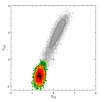
Figure 3: The ${\mbox{\boldmath$\pi$}}_{\rm E}$ contours at 1, 2, 3, and $4\,\sigma$ in black, red, orange, and green, respectively. As a comparison, the gray points show the approximate $3\sigma$ region of Model 4, i.e., with both parallax and orbital motion effects, with the $1\sigma$ contour shown in black. The black cross shows the (0,0) coordinates.

4.4 Orbital motion effects

For the planet orbital motion, we use the formalism of Dong et al. (2009a). The lightcurve is capable of constraining at most two additional orbital parameters that can be interpreted as the instantaneous velocity components in the plane of the sky. They are implemented via two new MCMC parameters $ds/dt$ and $\omega$, which are the uniform expansion rate in binary separation $s$ and the binary rotation rate $\alpha$,

$$s=s_{0}+ds/dt\,(t-t_{0})\\ \alpha=\alpha_{0}+\omega\,(t-t_{0}).$$ (11)

These two effects induce variations in the shape and orientation of the resonant caustic, respectively. To ensure that the resulting orbital characteristics are physically plausible, we can verify for any trial solution that the projected velocity of the planet is not greater than the escape velocity of the system, $v_{\perp}<v_{esc}$ for a given assumed mass and distance, where (Dong et al. 2009a)

$$v_{\perp}=\sqrt{(ds/dt)^{2}+(\omega s)^{2}}D_{l}\theta_{E}$$ (12)

and

$$v_{esc}=\sqrt{\frac{2GM}{r}}\leq v_{esc,\perp}=\sqrt{\frac{2GM}{r_{\perp}}},\qquad r_{\perp}=s\theta_{E}D_{l}.$$ (13)

The configuration with only orbital motion corresponds to the Model 3 of Table 1. The resulting diagram showing the solution for the two orbital parameters $\omega$ and $ds/dt$ is presented in Figure 4. Taking the orbital motion of the planet into account substantially improves the fit ($\Delta\chi^{2}=-67.5$).

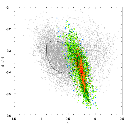
Figure 4: Orbital parameters of solutions at 1, 2, 3, and $4\,\sigma$ in black, red, orange, and green, respectively. As a comparison, the gray points show the $3\sigma$ region of Model 4, i.e., with both parallax and orbital motion effects, with the $1\sigma$ contour shown in black.

4.5 Combined parallax and orbital motion

In this section we model both parallax and orbital motion effects, which is called Model 4 in Table 1. Taking these two effects into account results in only a modest improvement in $\chi^{2}$ compared to the cases for which the effects are considered individually ($\chi^{2}_{both}-\chi^{2}_{orbital}=-9$). The triangle diagram presented in Figure 5 shows the 2-parameter contours between the four MCMC parameters $\pi_{\rm{E,N}}$, $\pi_{\rm{E,E}}$, $\omega$ and $ds/dt$ introduced in Sections 4.3 and 4.4. The best fit is $(\pi_{\rm{E,N}},\pi_{\rm{E,E}})=(2.495,-0.311)$ and $(\omega,ds/dt)=(-0.738,-0.360)$. This would lead to a host star of $0.015\,M_{\odot}$ at a distance $D_{l}=1.11$ kpc and a $0.21$ Jupiter mass planet with a projected separation of $0.32$ AU.

This small improvement in $\chi^{2}$ can be explained by a degeneracy between the north component of ${\mbox{\boldmath$\pi$}}_{\rm E}$ and the orbital parameter $\omega$, as shown in Figure 5. In fact, the actual degeneracy is between $\pi_{\rm{E},\perp}$ and $\omega$, where $\pi_{\rm{E},\perp}$ (described by Gould 2004) is the component of ${\mbox{\boldmath$\pi$}}_{\rm E}$ that is perpendicular to the instantaneous direction of the Earth’s acceleration, i.e., that of the Sun projected on the plane of the sky at the peak of the event. This acceleration direction is $\phi=257.4^{\circ}$ (north through east). Hence, the perpendicular direction is $\phi-90^{\circ}=192.6^{\circ}$, which is quite close to the $195.7^{\circ}$ degeneracy direction in the $\pi_{\rm{E,N}}$ and $\pi_{\rm{E,E}}$ diagram. Since $\pi_{\rm{E,\perp}}$ is very close (only $13^{\circ}$) from north, $\pi_{\rm{E,N}}$ is a good approximation for it.

Indeed, $\pi_{\rm{E,\parallel}}$ generates an asymmetry in the lightcurve because, to the extent that the source-lens motion is in the direction of the Sun-Earth axis, the event rises faster than it falls (or vice versa). This effect is relatively easy to detect. But to the extent that the motion is perpendicular to this axis, the Sun’s acceleration induces a parabolic deviation in the trajectory. To lowest order, this produces exactly the same effect as rotation of the lens geometry (which is a circular deviation). Hence, the degeneracy between $\pi_{\rm{E,\perp}}$ and $\omega$ can only be broken at higher order. This degeneracy was discussed in the context of point lenses in Gould, Miralda-Escude & Bahcall (1994), Smith, Mao & Paczyński (2003a), and Gould (2004). In the point-lens case, the $\pi_{\rm{E,\perp}}$ degeneracy appears nakedly (because the lens system is invariant under rotation). In the present case, the rotational symmetry is broken. In case orbital motion is ignored, it thus may appear that parallax is measured more easily in binary events, as originally suggested by An & Gould (2001). But in fact, as shown in the present case, once the caustic is allowed to “rotate” (lowest order representation of orbital motion), then the $\pi_{\rm{E,\perp}}$ degeneracy is restored.

4.6 Limb-darkening implementation

Most of the calculations in this paper are done using Stokes’ theorem, which greatly speeds up the computations by reducing a 2-dimensional integral to one dimension. However, this method implicitly assumes that the source has uniform surface brightness, whereas real sources are limb darkened. In the linear approximation, the normalized surface brightness can be written

$$W(z;\Gamma)=1-\Gamma\biggl{(}1-\frac{3}{2}\sqrt{1-z^{2}}\biggr{)},$$ (14)

where $\Gamma$ is the limb-darkening coefficient depending on the considered wavelength, and $z$ is the position on the source divided by the source radius.

We adopt this approach because we expect that the solutions with and without limb darkening will be nearly identical, except that the uniform source should appear smaller by approximately a factor

$${\rho_{\rm uni}\over\rho_{\rm ld}}\simeq\sqrt{\int dz^{2}z^{2}W(z:\Gamma)\bigg{/}\int dz^{2}z^{2}}=\sqrt{1-{\Gamma\over 5}}$$ (15)

because this ratio preserves the rms radial distribution of light.

To test this conjecture, we approximate the surface as a set of 20 equal-area rings, with the magnification of each ring still computed by Stokes’ method. The surface brightness of the $i$th ring is simply $W(z_{i})$ where $z_{i}$ is the middle of the ring. The limb-darkening coefficients for the unfiltered data have been determined by interpolation, from $V$, $R$, $I$ and $H$ limb-darkening coefficients. We find from the CMD that the source star has $(V-I)_{0}=0.82$, so roughly a G7 dwarf or slightly cooler. We adopt a temperature of $T=5500$ K. We thus obtain the following limb-darkening parameters $(u_{V},u_{R},u_{I},u_{H})=(0.7117,0.6353,0.5507,0.3659)$, where $u=3\Gamma/(\Gamma+2)$ (Afonso et al. 2000). Then $(\Gamma_{V},\Gamma_{R},\Gamma_{I},\Gamma_{H})=(0.6220,0.5373,0.4497,0.2778)$. For a given observatory/filter (or possibly unfiltered), we then compare $(R_{observed}-I_{CTIO})$ to $(V_{CTIO}-I_{CTIO})$, considering that $I_{CTIO}=0.07V+0.93I$ and that approximately $V=2R-I$ and deduce empirical expression for the corresponding $\Gamma$ coefficients. The $\Gamma$ coefficients for all the observatories then become $(\Gamma_{MOA},\Gamma_{SAAO},\Gamma_{FCO},\Gamma_{AO},\Gamma_{Danish},\Gamma_{Bronberg},\Gamma_{Wise})=(0.493,0.45,0.52,0.51,0.45,0.53,0.49)$. Substituting, a mean $\Gamma\sim 0.47$ into Eq. (15), we expect $\rho$ to be $\sim 5\%$ larger when limb-darkening is included.

4.7 Results summary

We summarize the best-fit results for the five different models presented in Section 4 in Table 1. The five models are Model 1: Finite-source binary-lens model with neither parallax nor orbital motion effects; Model 2: Finite-source binary-lens model with parallax effects only; Model 3: Finite-source binary-lens model with orbital motion effects only; Model 4: Finite-source binary-lens model with both parallax and orbital motion effects; and Model 5: Finite-source binary-lens model with both parallax and orbital motion effects and limb-darkening.

Note in particular that Models 4 and 5 agree within $\sim 1\,\sigma$ for all parameters, except that $\rho$ is $\sim 7\%$ greater in the limb-darkened case (Model 5).

5 Bayesian analysis

The Markov Chain used to find the solutions illustrated in Figure 5 is constructed (as usual) by taking trial steps that are uniform in the MCMC variables, including $t_{0}$, $u_{0}$, and $t_{\rm E}$. This amounts to assuming a uniform prior in each of these variables. In the case of the three variables $t_{0}$, $u_{0}$, and $t_{\rm E}$, the solution is extremely well constrained, so it makes hardly any difference which prior is assumed. Whenever this is the case, Bayesian and frequentist orientations lead to essentially the same results. However, as shown in Figure 5, $\@vec{\pi}_{\rm E}$ is quite poorly constrained: at the $2\sigma$ level, the magnitude of $\pi_{\rm E}$ varies by more than an order of magnitude. Since the lens distance is related to the microlens parallax by $D_{l}={\rm AU}/(\theta_{\rm E}\pi_{\rm E}+\pi_{S})$, where $\pi_{S}={\rm AU}/D_{s}$, this amounts to giving equal prior weight to a tiny range of distances nearby and a huge range of distances far away. But the actual weighting should have the reverse sign, primarily because a fixed distance range corresponds to far more volume at large than small distances. In fact, a Galactic model should be used to predict the a priori expected rate of microlensing events, which depends not only on the correct volume element but also on the density and velocity distributions of the lens and the source as well.

Similarly, a Keplerian orbit can be equally well characterized by specifying the seven standard Kepler parameters or six phase-space coordinates at a given instant of time, plus the host mass. The latter parametrization is more convenient from a microlensing perspective because microlensing most robustly measures the two in-sky-plane Cartesian spatial coordinates ($s\cos\alpha$ and $s\sin\alpha$) and the two in-plane Cartesian velocity coordinates ($ds/dt$ and $s\omega$), while the mass is directly given by microlens variables $M=\theta_{\rm E}/\kappa\pi_{\rm E}$. However, the former (Kepler) variables have simple well-established priors. By stepping equally in microlens parameters, one is effectively assuming uniform priors in these variables, whereas one should establish the priors according to the Kepler parameters.

In principle, one would simultaneously incorporate both sets of priors (Galactic and Kepler), and we do ultimately adopt this approach. However, it is instructive to first apply them separately to determine whether these two sets of priors are basically compatible or are relatively inconsistent.

Figure 5: Parallax and orbital motion parameters of solutions contours at 1, 2, 3, and $4\,\sigma$. The black crosses show the (0,0) coordinates.

Table 1. Fit parameters for finite-source binary-lens models
Model	$t_{0}$	$u_{0}$	$t_{E}$	$s$	$q$	$\alpha$	$\rho$	$\pi_{E,N}$	$\pi_{E,E}$	$\omega$	$ds/dt$
$\chi^{2}$	Error bars
Model 1	5042.34	0.0683	48.7	0.9152	0.01073	4.3074	0.00149	-	-	-	-
1100	0.01	0.0005	0.4	0.0002	0.00015	0.0025	0.00002	-	-	-	-
Model 2	5042.38	0.0770	43.9	0.9137	0.01230	4.3063	0.00174	-1.38	0.60	-	-
1048	0.02	0.0015	0.5	0.0004	0.00030	0.0030	0.00005	0.25	0.07	-	-
Model 3	5042.32	0.0902	38.4	0.9137	0.0135	4.302	0.00197	-	-	-0.252	-0.409
1032.5	0.02	0.002	0.6	0.0003	0.0002	0.002	0.00005	-	-	0.1	0.04
Model 4	5042.366	0.0890	40.1	0.9134	0.0135	4.3095	0.00195	2.5	-0.31	-0.74	-0.36
1024.5	0.015	0.0010	0.5	0.0002	0.0002	0.0025	0.00003	1	0.3	0.2	0.05
Model 5	5042.36	0.0881	40.0	0.9136	0.0132	4.3099	0.00202	1.7	-0.15	-0.51	-0.37
1029.2	0.02	0.0010	0.5	0.0003	0.0002	0.0025	0.00003	1	0.5	0.3	0.05

Formally, we can evaluate the posterior distribution $f(X\mid D)$, including both prior expectations from (Galactic and/or Keplerian) models and posterior observational data using Bayes’ Theorem :

$$f(X\mid D)=\frac{f(D\mid X)f(X)}{f(D)}.$$ (16)

Here $f(D\mid X)$ is the likelihood function over the data $D$ for a given model $X$, $f(X)$ is the prior distribution containing all ex ante information about the parameters $X$ available before observing the data, and $f(D)=\int_{X}f(D\mid X)f(X)dX$. In the present context, this standard Bayes formula is interpreted as follows: the density of links on the MCMC chain directly gives $f(D\mid X)$, while $f(X)$ encapsulates the parameter priors, including both the underlying rate of events in a “natural physical coordinate system” in which these priors assume a simple form and the Jacobian of the transformation from this “physical” system to the “natural microlensing parameters” that are directly modeled in the lightcurve analysis.

It is not obvious, but we find below that the coordinate transformations for Galactic and Kepler models actually factor, so we can consider them independently.

5.1 Galactic model

Applying the generic rate formula $\Gamma=n\sigma v$ to microlensing rates as a function of the independent physical variables $(M,D_{l},{\mbox{\boldmath$\mu$}})$, yields

$$f_{\rm Gal}(X)\propto\frac{d^{4}\Gamma}{dD_{L}\,dM\,d^{2}\mu}=\nu(x,y,z)(2R_{\rm E})v_{\rm{rel}}f({\mbox{\boldmath$\mu$}})g(M),$$ (17)

where the spatial positions $(x,y,z)$, the physical Einstein radius $R_{\rm E}$, and the lens velocity relative to the observer-source line of sight $v_{\rm{rel}}$ are all regarded as dependent variables of the four variables shown on the l.h.s., plus the two angular coordinates. Here $\nu(x,y,z)$ is the local density of lenses, $g(M)$ is the mass function [we will eventually adopt $g(M)\propto M^{-1}$], and $f({\mbox{\boldmath$\mu$}})$ is the two-dimensional probability function for a given source-lens relative proper motion, $\mu$. Since $v_{\rm{rel}}=\mu D_{l}$ and $R_{\rm E}=D_{l}\theta_{\rm E}$, this can be rewritten in terms of microlensing variables,

$${d^{4}\Gamma\over dt_{\rm E}\,d\theta_{\rm E}\,d^{2}\pi_{\rm E}}={d^{4}\Gamma\over dD_{L}\,dM\,d^{2}\mu}\,\times{\mu\over\pi_{\rm E}}\bigg{|}{\partial(D_{L},M,\mu)\over\partial(t_{\rm E},\theta_{\rm E},\pi_{\rm E})}\bigg{|}$$

$$=2D_{l}^{2}\theta_{\rm E}\mu\nu(x,y,z)f({\mbox{\boldmath$\mu$}})g(M)\times{2\over{\rm AU}}D_{l}^{2}{M\,\pi_{\rm{rel}}\,\mu^{2}\over t_{\rm E}\theta_{\rm E}\pi_{\rm E}^{2}},$$

where $M=\theta_{\rm E}/\kappa\pi_{\rm E}$, $D_{l}={\rm AU}/(\pi_{\rm{rel}}+\pi_{s})$, $\pi_{\rm{rel}}=\theta_{\rm E}\pi_{\rm E}$, and $\mu=\theta_{\rm E}/t_{\rm E}$ are now regarded as dependent variables. We note that

$${\partial(D_{L},M,\mu)\over\partial(t_{\rm E},\theta_{\rm E},\pi_{\rm E})}={\partial(\pi_{\rm{rel}},M,\mu)\over\partial(t_{\rm E},\theta_{\rm E},\pi_{\rm E})}{dD_{L}\over d\pi_{\rm{rel}}}={2\pi_{\rm{rel}}\,M\,\mu\over t_{E}\,\theta_{\rm E}\,\pi_{\rm E}}{D_{L}^{2}\over{\rm AU}},$$

where the last evaluation follows from the general theorem:

$$y_{i}=\prod_{j}x_{j}^{\alpha_{ij}}\Longrightarrow{\partial(y_{i})\over\partial(x_{j})}={\partial(\ln y_{i})\over\partial(\ln x_{j})}{\prod_{i}y_{i}\over\prod_{j}x_{j}}=|\alpha|{\prod_{i}y_{i}\over\prod_{j}x_{j}}.$$

Finally, Eq. (17) reduces to

$${d^{4}\Gamma\over dt_{\rm E}\,d\theta_{\rm E}\,d^{2}\pi_{\rm E}}={4\over\rm AU}\nu(x,y,z)f({\mbox{\boldmath$\mu$}})[g(M)M]{D_{l}^{4}\mu^{4}\over\pi_{\rm E}}.$$ (18)

The variables on the l.h.s. of Eq. (18) are essentially the Markov chain variables in the microlensing fit procedure. The distribution of MCMC links applied to the data can be thought of as the posterior probability distribution of the Markov-chain variables under the assumption that the prior probability distribution in these variables is uniform. In our case, the prior distribution is not uniform, but is instead given by the r.h.s. of Eq. (18). We therefore must weight the output of the MCMC by this quantity, which is the specific evaluation of $f(X)$ in Eqs. (16) and (17).

As mentioned above, we adopt $g(M)\propto M^{-1}$, so the term in square brackets disappears. We evaluate $\nu(x,y,z)$ and $f({\mbox{\boldmath$\mu$}})$ as follows.

5.1.1 Lens-source relative proper motion distribution $f({\mbox{\boldmath$\mu$}})$

To compute the relative proper motion probability, we assume that the velocity distributions of the lenses and sources are Gaussian $f(v_{y},v_{z})=f(v_{y})f(v_{z})$ where

$$f(\mu_{y})=f(v_{y})\frac{dv_{y}}{d\mu_{y}}=D_{L}\frac{1}{\sqrt{2\pi\sigma_{y}^{2}}}\rm{exp}\bigg{[}-\frac{(v_{y}-\tilde{v}_{y})^{2}}{2\tilde{\sigma_{y}}^{2}}\bigg{]}$$ (19)

and a similar distribution for $f(\mu_{z})$. Here $v_{y}$ and $v_{z}$ are components of the projected velocity $\@vec{v}$ derived from the MCMC fit, which is expressed by $\@vec{v}=\@vec{\mu}D_{l}$, where

$$\@vec{\mu}=\frac{\@vec{\pi_{E}}}{\pi_{E}}\frac{\theta_{E}}{t_{E}}.$$ (20)

The expected projected velocity which appears in Eq.19 is defined as

$$\mbox{\boldmath$\tilde{v}$}=\mbox{\boldmath$v_{l}$}-\Bigg{[}\mbox{\boldmath$v_{s}$}\frac{D_{l}}{D_{s}}+\mbox{\boldmath$v_{o}$}\frac{D_{ls}}{D_{s}}\Bigg{]}$$ (21)

where $D_{l}$, $D_{s}$ are respectively the lens and source distances from the observer and $D_{ls}$ the lens-source distance. The velocity is expressed in the $(x,y,z)$ coordinate system, centered on the center of the Galaxy, where $x$ and $z$ axes point to the Earth and the North Galactic pole, respectively. As given in Han & Gould (1995), we adopt $\@vec{v}_{z,disk}=\@vec{v}_{z,bulge}=0$ and $\sigma_{z,disk}=20\,\rm{km.s}^{-1}$, $\sigma_{z,bulge}=100\,\rm{km.s}^{-1}$ for the $z$ component of the velocity. For the $y$ direction, $\@vec{v}_{y,disk}=220\,\rm{km.s}^{-1}$, $\@vec{v}_{y,bulge}=0$ and $\sigma_{y,disk}=30\,\rm{km.s}^{-1}$, $\sigma_{y,bulge}=100\,\rm{km.s}^{-1}$ depending on whether the lens is situated in the disk or in the bulge. We also consider the asymmetric drift of the disk stars by subtracting $10\,\rm{km.s}^{-1}$ from $\@vec{v}_{y,disk}$. The celestial north and east velocities of the Earth seen by the Sun at the time of the event are $\@vec{v}_{E}=(v_{E,E},v_{E,N})=(+22.95,-3.60)\,\rm{km.s}^{-1}$. In the Galactic frame, the galactic north and east components of the Earth velocity become

$$v_{\rm E,North\,Gal}=v_{E,N}\cos{59.7^{\circ}}-v_{E,E}\sin{59.7^{\circ}},$$ (22)

$$v_{\rm E,East\,Gal}=v_{E,N}\sin{59.7^{\circ}}+v_{E,E}\cos{59.7^{\circ}}.$$ (23)

The velocity of the Sun in the Galactic frame is $\@vec{v}_{\odot}=(7,12)\,\rm{km.s}^{-1}+(0,v_{\rm{circ}})$, where $v_{\rm{circ}}=220\,\rm{km.s}^{-1}$, from which we deduce the velocity $v_{o}$ of the observer in the Galactic frame by adding the Earth velocity from Eq. (22).

5.1.2 Density distribution $\nu(x,y,z)$

The density distribution, $\nu(x,y,z)$, is given at the lens coordinates (x,y,z) in the Galactic frame. For this distribution, we adopt the model of Han & Gould (2003), which is based primarily on star counts, and, without any adjustment, reproduces the microlensing optical depth measured toward Baade’s window. The density models are given in Table 5.3. The disk parameters are $H=2.75\,$kpc, $h_{1}=156\,$pc, $h_{2}=439\,$pc, and $\beta=0.381$, where $R\equiv(x^{2}+y^{2})^{1/2}$. For the barred (anisotropic) bulge model, $r_{s}=\big{(}[(x^{\prime}/x_{0})^{2}+(y^{\prime}/y_{0})^{2}]^{2}+(z^{\prime}/z_{0})^{4}\big{)}^{1/4}$. Here the coordinates $(x^{\prime},y^{\prime},z^{\prime})$ have their center at the Galactic center, the longest axis is the $x^{\prime}$, which is rotated $20^{\circ}$ from the Sun-GC axis toward positive longitude, and the shortest axis is the $z^{\prime}$ axis. The values of the scale lengths are $x_{0}=1.58$ kpc, $y_{0}=0.62$ kpc and $z_{0}=0.43$ kpc respectively. For the bulge, Han & Gould (2003) normalize the “G2” K-band integrated-light-based bar model of Dwek et al. (1995) using star counts toward Baade’s window from Holtzman et al. (1998) and Zoccali et al. (2000). For the disk, they incorporate the model of Zheng et al. (2001), which is a fit to star counts.

In the calculation, we sum the probabilities of disk and bulge locations for the lens. We set the limits of the disk range to be $[0,7]$ kpc from us and $[5,11]$ kpc for the bulge range. We also apply the bulge density distribution to the source, in the $[6.5,11]$ kpc range. Rigorously, because we already know the dereddened flux of the source, we should have derived a distribution of sources from the luminosity distribution of bulge stars combined with their distance. However, as we do not know the precise distribution of bulge luminosities at fixed color, we only consider the density distribution of sources as a function of their position in the bulge only. Because the stellar density drops off very rapidly from the peak, the source is effectively localized as being close to the Galactocentric distance.

5.2 Orbital motion model

In addition to the Galactic model, we build a Keplerian model to put priors on the orbital motion of the planet. To extract the orbital parameters from the microlensing parameters, we refer to the appendix of Dong et al. (2009a). Given that from the light curve of the event we have access to the instantaneous projected velocity and position of the planet for only a short time, we consider a circular orbit to model the planet motion. The distortions of the light curve are modeled by $\omega$ and $ds/dt$, which then specify the variations in orientation and shape of the resonant caustic, respectively. These quantities are defined in Section 4.4. Since $r_{\perp}=D_{l}\theta_{E}d$ is the projected star-planet separation, we evaluate the instantaneous planet velocity in the sky plane, with $r_{\perp}\gamma_{\perp}=r_{\perp}\omega$ the velocity perpendicular to the planet-star axis and $r_{\perp}\gamma_{\parallel}=r_{\perp}(ds/dt)/s$ the velocity parallel to this axis. We define the $\hat{i},\hat{j},\hat{k}$ directions as the instantaneous star-planet axis on the sky plane, the direction into the sky, and $\hat{k}=\hat{i}\times\hat{j}$. In this frame, the planet is moving among two directions, defined by the angles $\theta$ and $\phi$, which are effectively a (complement to a) polar angle and an azimuthal angle, respectively. Specifically, $\phi$ is the angle between the star-planet-observer ($r_{\perp}=a\sin\phi$), and $\theta$ characterizes the motion in the direction of the velocity along $\hat{k}$. Then the instantaneous velocity of the planet is

$$v=\sqrt{\frac{GM}{a}}[\cos\theta\hat{k}+\sin\theta(\cos\phi\hat{i}-\sin\phi\hat{j})]$$ (24)

where $a$ is the semimajor axis. Thus we obtain $\gamma_{\perp}=\sqrt{\frac{GM}{a^{3}}}\frac{\cos\theta}{\sin\phi}$ and $\gamma_{\parallel}=\sqrt{\frac{GM}{a^{3}}}\sin\theta\cot\phi$. The Jacobian expression to transform from $P(s,\gamma_{\perp},\gamma_{\parallel})$ to $P(a,\phi,\theta)$ is

$$J={\partial(a,\phi,\theta)\over\partial(s,\gamma_{\perp},\gamma_{\parallel})}={a^{3}\over GM}\tan^{2}\phi\big{(}\frac{1}{2}-\sin^{2}\theta\tan^{2}\phi\big{)}^{-1}R_{\rm E}$$ (25)

As explained in Dong et al. (2009a), for one set of microlensing parameters, there are two degenerate solutions in physical space. In the orbital model, we consider the two solutions to constrain the light curve fit, each with its own separate probability.

From the definition of the two angles, the transformation of the polar system $(a,\pi/2-\theta,\phi)$ contains the quantity $\sin\theta$ and so the Jacobian includes the factor $\cos\theta$ from $d(\sin\theta)d\phi=d\theta d\phi\cos\theta$. Moreover, we adopt a flat distribution on $\ln(a)$, implying the factor $1/a$ in the Jacobian expression. Then,

$$J=\frac{\partial(\ln(a),\phi,\sin\theta)}{\partial(s,\gamma_{\perp},\gamma_{\parallel})}=\frac{r^{2}_{\perp}}{GM}\frac{\cos\theta}{\cos^{2}\phi}\big{(}\frac{1}{2}-\sin^{2}\theta\tan^{2}\phi\big{)}^{-1}R_{\rm E}$$ (26)

Note that the terms $\sin\theta$ and $\cos\theta$ in the denominators of Eq. (26) correct an error in Dong et al. (2009a).

5.3 Constraints from VLT

As foreshadowed in Section 2.1, the VLT NACO flux measurement places upper limits on the flux from the lens, hence on its mass (assuming it is not a white dwarf). However, we begin by assuming that the excess light is caused by the lens. We do so for two reasons. First, this is actually the most precise way to enforce an upper limit on the lens flux. Second, it is of some interest to see what mass range is “picked out” by this measurement, assuming the excess flux is due to the lens.

The first point to note is that, if the lens contributes any significant flux, then it lies behind most or all of the dust seen toward the source. For example, if the lens mass is just $M=0.15\,M_{\odot}$ (which would make it quite dim, $M_{H}>8$), then it would lie at distance $D_{L}={\rm AU}/(\theta_{\rm E}^{2}/\kappa M+{\rm AU}/D_{S})=4.9\,$kpc, where we have adopted the central values $\theta_{\rm E}=0.31\,$mas and $D_{S}=8.7\,$kpc for this exercise. More massive lenses would be farther.

Next we estimate $A_{H}=0.4$ from the measured clump color $(V-I)_{\rm cl}=2.10$, assuming an intrinsic color of the red giant clump of $(V-I)_{0,\rm cl}=1.08$ (Bensby et al. 2010) and adopting for this line of sight $A_{H}/E(V-I)=0.40$.

Finally, for the relation between $M$ and $M_{H}$, we consult the library of empirically-calibrated isochrones of An et al. (2007). We adopt the oldest isochrones available (4 Gyr), since there is virtually no evolution after this age for the mass range that will prove to be of interest $M<0.7\,M_{\odot}$. Moreover, in this mass range, the isochrones hardly depend on metallicity within the range explored ($-0.3<{\rm[Fe/H]}<+0.2$).

Table 2. Density distribution for the bulge and disk models
Location	Model	Distribution (in $M_{\odot}\,{\rm pc}^{-3}$)
Bulge	Dwek	$\nu(r_{s})=1.23\exp(-0.5r^{2}_{s})$
Disk	Zheng	$\nu(R,\,z)=1.07\,\exp(-R/H)[(1-\beta)(-|z|/h_{1})+\beta\exp(-z/h_{2})]$

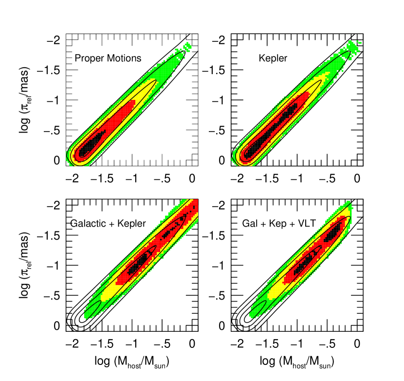
Figure 6: Bayesian analysis results. Each panel shows host mass $M$ versus lens-source relative parallax $\pi_{\rm rel}$, with 1, 2, 3, and $4\,\sigma$ contours under two different conditions. The solid black contours are derived from the light curve alone, without any priors. The colored symbols show contour levels after applying various priors, respectively Galactic proper motion only, Kepler only, full Galactic and Kepler priors, and full Galactic and Kepler priors, plus VLT imaging constraints. The proper-motion and Kepler priors are fully consistent with the light curve, but there is strong tension between between the distance-related priors and the lightcurve, with the former favoring high masses and small lens-source separations. The highest part of this disputed mass range, $M>0.7\,M_{\odot}$, is essentially ruled out by the VLT imaging constraint (lower right).

For each mass and distance considered below, we then calculate $H_{L}=M_{H}+A_{H}+5\log(D_{L}/10\,{\rm pc})$ and combine the corresponding flux with $H_{S}=18.35$ to obtain $H_{\rm pred}$. We then calculate a likelihood factor $L_{H}=\exp[-(H_{\rm pred}-H_{\rm obs})^{2}/2\sigma_{H}^{2}]$, where $H_{\rm obs}=18.25$ and $\sigma_{H}=0.07$, as discussed in Section 2.1.

For fiducial values $D_{S}=8.7\,$kpc and $\theta_{\rm E}=0.31\,$mas, this likelihood peaks at $M=0.42\,M_{\odot}$, but it does so very gently. The suppression factor is just $L_{H}\sim 0.7$ at $M=0.21\,M_{\odot}$ and $M=0.52\,M_{\odot}$. At lower masses, even if there were zero flux, the suppression would never get lower than $L_{H}=0.36$, simply because the excess-flux measurement is consistent with zero at $1.4\,\sigma$. But at higher mass, the expected flux quickly becomes inconsistent. For example, $L_{H}(0.65\,M_{\odot})=0.07$.

Hence, by treating the flux measurement as an excess-flux “detection”, we impose the “upper limit” on mass in a graceful manner. Moreover, as regards the upper limit, this approach remains valid when we relax the assumption that the excess flux is solely due to the lens. That is, even if there are other contributors, the likelihood of a given high-mass lens being compatible with the flux measurement can only go down.

However, the same reasoning does not apply at the low-mass limit. For example, if the excess flux came from a source companion or an ambient star, then a brown-dwarf lens would be fully compatible with the flux measurement. Nevertheless, this is quite a minor effect because, in any event, the suppression factor would not fall below 0.36. To account for other potential sources of light, we impose a minimum suppression factor $L_{H,{\rm min}}=0.5$ at the low-mass end.

5.4 Combining Galactic and Kepler priors and adding VLT constraints

In this section, we impose the priors from the Galactic and Kepler models and add the constraints from the VLT flux measurement. We defer the VLT constraints to the end because they do not apply to the special case of white-dwarf lenses.

We begin by examining the role of the various priors separately to determine the level of “tension” between these and the $\chi^{2}$ derived from the light curve alone. We do so because each prior involves different physical assumptions, and tension with the light curve may reveal shortcomings in these assumptions.

The Kepler priors involve two assumptions, first that the planetary system is viewed at a random orientation (which is almost certainly correct) and second that the orbit is circular (which is almost certainly not correct). We will argue further below that the assumption of circular orbits has a modest impact. In any event, we want to implement the Kepler priors by themselves.

The Galactic priors really involve two sets of assumptions. The more sweeping assumption is that planetary systems are distributed with the same physical-location distribution and host-mass distribution as are stars in the Galaxy. We really have no idea whether this assumption is true or not. For example, it could be that bulge stars do not host planets. The assumptions about host mass and physical location are linked extremely strongly in a mathematical sense (even if they prove to be unrelated physically) because $\theta_{\rm E}$ is well-measured, and $\theta_{\rm E}^{2}=\kappa M\,\pi_{\rm rel}$. Thus, we must be cautious about this entire set of assumptions.

However, the Galactic priors also contain another factor $f({\mbox{\boldmath$\mu$}})$, in which we can have greater a priori confidence. This prior basically assumes that planetary systems at a given distance (regardless of how common they are at that distance) will have similar kinematics to the general stellar population at the same distance. The scenarios in which this assumption would be strongly violated, while not impossible, are fairly extreme.

Therefore we begin by imposing proper-motion-only and Kepler-only priors in the top two panels of Figure 6, which plots host mass $M$ versus lens-source relative parallax $\pi_{\rm rel}$. We choose to plot $\pi_{\rm rel}$ rather than $D_{L}$ because it is given directly by microlensing parameters $\pi_{\rm rel}=\pi_{\rm E}\theta_{\rm E}$. The 1, 2, 3, and 4 $\sigma$ contours from the $\chi^{2}$ based on the light curve only are shown in black. Each of these priors is consistent with the light curve at the $1\,\sigma$ level, so we combine them and find that they still display good consistency. In the lower left panel, we combine the full Galactic and Kepler priors. These tend to favor much heavier, more distant lenses, which are strongly disfavored by the lightcurve, primarily because of the factor $D_{l}^{4}/\pi_{\rm rel}$ in Eq. (18). Indeed masses $M>0.7\,M_{\odot}$ will be effectively ruled out by high-resolution VLT imaging, further below.

When combining Galactic and Kepler priors, we simply weight the output of the MCMC by the product of the factors corresponding to each. This is appropriate because, while the $6\times 6$ matrix, transforming the full set of microlensing parameters $(s,\gamma_{\perp},\gamma_{\parallel},t_{E},\theta_{E},\pi_{E})$ to the full set of physical parameters $(a,\phi,\theta,M,D_{L},\mu)$, is not block diagonal, the Jacobian nevertheless factors as

$$\frac{\partial(a,\phi,\theta,M,D_{L},\mu)}{\partial(s,\gamma_{\perp},\gamma_{\parallel},t_{E},\theta_{E},\pi_{E})}=\frac{\partial(a,\phi,\theta)}{\partial(s,\gamma_{\perp},\gamma_{\parallel})}\times\frac{\partial(M,D_{L},\mu)}{\partial(t_{E},\theta_{E},\pi_{E})}.$$

Hence, the full weight, $f(X)$ in Eq. (16) is simply the product of the two found separately for the Galactic and orbital priors.

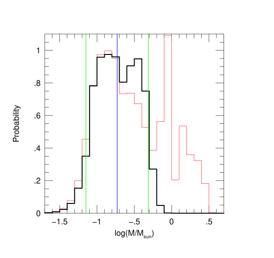
Figure 7: Probability as a function of host mass after applying the Galactic and Kepler priors (red) and then adding the constraints from VLT observations (black).

Figure 7 shows the host-mass probability distribution before (red) and after (black) applying the constraint from VLT imaging to the previous analysis incorporating both Galactic and Kepler priors. The 90% confidence interval is marked. The high mass solutions toward the right are strongly disfavored by the lightcurve (see Figure 6), but the Galactic prior for them is so strong that they have substantial posterior probability. However, these solutions are heavily suppressed by the VLT flux limits. The hsot is most likely to be an M dwarf. The lower right panel of Figure 6 shows the 2-dimensional $(M,\pi_{\rm rel})$ probability distribution for direct comparison with the results from applying various combinations of priors.

5.5 Bayesian results for physical parameters

Table 3 shows the median estimates and 90% confidence intervals for six physical parameters (plus one physical diagnostic) as more priors and constraints are applied. The bottom row, which includes full Galactic and Kepler priors, plus constraints from VLT photometry shows our adopted results. The six physical parameters are the host mass $M$, the planet mass $m_{p}$, the distance of the system $D_{L}$, the period $P$, the semi-major axis $a$, and the orbital inclination $i$. The last three assume a circular orbit. For rows 2 and 4 (which do not apply Kepler constraints), the values shown for $(P,a,i)$ summarize the results restricted to links in the chain that are consistent with a circular orbit, while the first four columns summarize all links in the chain. The key results are

$$0.071\,M_{\odot}<M_{\rm host}<0.49\,M_{\odot}\qquad(90\%\ \rm confidence)$$ (27)

and corresponding to this, $m_{p}=qM$, where $q=0.00132\pm 0.00002$, i.e.,

$$1.0\,M_{\rm Jup}<m_{p}<6.7\,M_{\rm Jup}\qquad(90\%\ \rm confidence),$$ (28)

$$3.8\,{\rm yr}<P<7.6\,{\rm yr}\qquad(90\%\ \rm confidence)$$ (29)

$$1.1\,{\rm AU}<a<2.7\,{\rm AU}\qquad(90\%\ \rm confidence)$$ (30)

with the medians at $M=0.19\,M_{\odot}$, $m_{p}=2.6\,M_{\rm Jup}$, $P=5.4\,$yr, $a=1.8\,$AU. That is, the host is an M dwarf with a super-Jovian massive planetary companion. For completeness, we note that in obtaining these results, we have implicitly assumed that the probability of a star having a planet with a given planet-star mass ratio $q$ and semi-major axis $a$ is independent of the host mass and distance.

5.6 White dwarf host?

When we applied the VLT flux constraint, we noticed that it would not apply to white-dwarf hosts. Is such a host otherwise permitted? In principle, the answer is “yes”, but as we now show, it is rather unlikely. The WD mass function peaks at about $M\sim 0.6\,M_{\odot}$, which corresponds to an $M_{\rm prog}\sim 2\,M_{\odot}$ progenitor. If the progenitor had a planet, it would have increased its semi-major axis by a factor $a/a_{\rm init}=M_{\rm prog}/M\sim 3.3$ as the host adiabatically expelled its envelope. We find that, for $M=0.6\,M_{\odot}$, the orbital semi-major axis is fairly tightly constrained to $a=2.3\pm 0.3\,$AU, implying $a_{\rm init}=0.7\pm 0.1\,$AU. It is unlikely that such a close planet would survive the AGB phase of stellar evolution. Of course, a white dwarf need not be right at the peak. For lower mass progenitors, the ratio of initial to final masses is lower, which would enhance the probability of survival. But it is also the case that such white dwarfs are rarer.

5.7 Physical consistency checks of bayesian analysis

The results reported here have been derived with the aid of fairly complicated machinery, both in fitting the light curves and in transforming from microlensing to physical parameters. In particular, we have identified a strong mathematical degeneracy between the parameters $\pi_{\rm E,N}$ and $\omega$, which arise from orbital motion of the Earth and the planet, respectively. When considering “MCMC-only” solutions, this degeneracy led to extremely large errors in $\pi_{\rm E,N}$ in Figure 5, which are then reflected in similarly large errors in the “light-curve-only” contours for host mass and lens-source relative parallax in Figure 6. Nevertheless, these large errors gradually shrink when the priors are applied in Figure 6, and more so when the constraints from VLT observations are added in Figure 7.

We have emphasized that the high-$\pi_{\rm E}$ (so low-$D_{L}$, low-$M$) solutions are very strongly, and improperly, favored by the MCMC when it is cast in microlensing parameters, and that the Galactic prior (Eq. 18) properly compensates for this. But is this really true? The best-fit distance for the Galactic-prior model is four times larger than for the MCMC-only model, meaning that the term $D_{\rm L}^{4}/\pi_{\rm rel}$ favors the Galactic model by a factor $\sim 2500$. Thus, even if the light curve strongly favored the nearby model, the Galactic prior could “trump” the light curve and enforce a larger distance. Indeed, this would be an issue if the Galactic prior were operating by itself. In fact, however, Figure 6 shows that the finally adopted solution (including the VLT flux constraint) is disfavored by the light curve alone by just $\Delta\chi^{2}\sim 3$, so, in the end there is no strong tension.

A second issue is that both parallax and orbital motion are fairly subtle effects that could, in principle, be affected by systematics. If this were the case, the principal lensing parameters, such as $q$ and $s$, would remain secure, but most of the “higher order” information, such as lens mass, distance, and orbital motion would be compromised. It is always difficult to test for systematics, particularly in this case for which there are two effects that are degenerate with each other and in combination are detected at only $\Delta\chi^{2}<100$.

Table 3. Physical parameters
Model	$M$	$m_{p}$	$D_{L}$	$E_{\rm kin}/E_{\rm pot}$	$P$	$a$	$i$
	$M_{\odot}$	$M_{\rm Jup}$	kpc		yr	AU	deg
Kepler	0.04	0.51	2.29	0.34	2.92	1.39	39
90% conf	$(0.01,0.12)$	$(0.19,1.69)$	$(0.98,4.79)$	$(0.07,0.44)$	$(1.37,5.42)$	$(0.18,2.10)$	$(24,74)$
Galactic	0.31	4.38	6.83	0.54	3.73	2.12	60
90% conf	$(0.07,6.37)$	$(1.03,89.61)$	$(3.65,9.37)$	$(0.06,1.81)$	$(1.37,6.26)$	$(1.06,3.01)$	$(40,79)$
Gal+Kep	0.28	3.82	6.44	0.28	4.99	2.04	50
90% conf	$(0.07,2.22)$	$(1.00,30.82)$	$(3.59,9.38)$	$(0.09,0.37)$	$(2.68,7.27)$	$(1.11,3.04)$	$(38,72)$
Gal+VLT	0.25	3.55	6.42	0.69	4.90	1.62	58
90% conf	$(0.07,0.53)$	$(1.04,7.52)$	$(3.62,8.34)$	$(0.12,1.99)$	$(3.50,6.79)$	$(0.98,2.45)$	$(42,84)$
G+K+VLT	0.19	2.56	5.69	0.27	5.43	1.82	52
90% conf	$(0.07,0.49)$	$(0.98,6.71)$	$(3.50,7.87)$	$(0.10,0.36)$	$(3.82,7.58)$	$(1.09,2.68)$	$(40,72)$

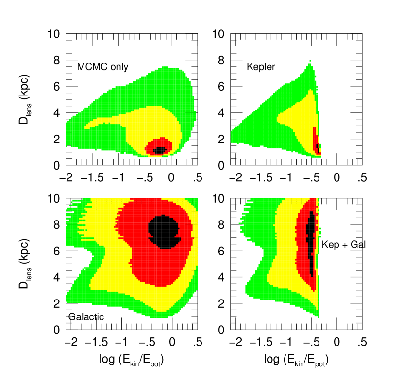
Figure 8: Physical test of Bayesian results: physicality diagnostic $\beta=E_{{\rm kin},\perp}/E_{{\rm pot},\perp}$ is plotted against host distance. Bound orbits must have $\beta<1$, and we expect a priori $0.1<\beta<0.5$.

However, we can in fact test for such systematics using the diagnostic

$$\beta\equiv{v_{\perp}^{2}\over v_{{\rm esc},\perp}^{2}}={E_{{\rm kin},\perp}\over E_{{\rm pot},\perp}},$$ (31)

where $v_{\perp}$ and $v_{{\rm esc},\perp}$ are defined in Eqs. (12) and (13). Bound orbits require $\beta<1$. Circular orbits, if seen face-on, have $\beta=0.5$ and otherwise $\beta<0.5$. Of course, it is possible to have $\beta\ll 1$, but it requires very special configurations to achieve this. For example, if the planet is close to transiting its host, or if the orbit is edge-on and the phase is near quadrature. Thus, a clear signature of systematics would be $\beta>1$ for all light-curve solutions with reasonable $\chi^{2}$. And if $\beta\la 0.1$, one should be concerned about systematics, although this condition would certainly not be proof of systematics. With these considerations in mind, we plot $D_{\rm L}$ vs. $\beta$ in Figure 8.

The key point is that the $1\,\sigma$ region of the Galactic-prior panel straddles the region $\beta\la 0.5$ ($\log\beta\la-0.7$), which is characteristic of approximately circular, approximately face-on orbits. It is important to emphasize that no selection or weighting by orbital characteristics has gone into construction of this panel. This is a test which could easily have been failed if the orbital parameters were seriously influenced by systematics: $\beta$ could have taken literally on any value.

Finally, we turn to the two righthand panels, which incorporate the orbital constraints. Since these assume circular orbits, they naturally eliminate all solutions with $\beta>0.5$, and some smaller-$\beta$ solutions as well, because when $ds/dt\not=0$, it is impossible to accommodate a $\beta=0.5$ circular orbit. While this radical censoring of the high-$\beta$ solutions is the most dramatic aspect of these plots, there is also the very interesting effect that low-$\beta$ solutions are also suppressed (though more gently). This is because, as mentioned above, these require special configurations and so are disfavored by the Kepler Jacobian, Eq. (25). Of course, radical censorship of $\beta>1$ solutions is entirely appropriate (provided that $\beta<1$ solutions exist at reasonable $\chi^{2}$), but what about $0.5\la\beta<1$? A more sophisticated approach would permit non-circular orbits and then suppress these solutions “more gently” using a Jacobian (as is already being for done low-$\beta$ solutions). However, as we have emphasized, the limited sensitivity of this event to additional orbital parameters does not warrant such an approach. Hence, radical truncation is a reasonable proxy in the present case for the “gentler” and more sophisticated approach.

Moreover, one can see by comparing Rows 2 and 3 of Table 3 that the addition of Kepler priors does not markedly alter the Galactic-prior solutions.

6 Conclusions

We report the discovery of the planetary event MOA-2009-BLG-387Lb. The planet/star mass ratio is very well-determined, $q=0.0132\pm 0.0003$. We constrain the host mass to lie in the interval. $0.07<M_{\rm host}/M_{\odot}<0.49$ at 90% confidence, which corresponds to the full range of M dwarfs. The planet mass therefore lies in the range $1.0<m_{p}/M_{\rm Jup}<6.7$ , with its uncertainty almost entirely due to the uncertainty in the host mass. The host mass is determined from two “higher-order” microlensing parameters, $\theta_{\rm E}$ and ${\mbox{\boldmath$\pi$}}_{\rm E}$, (i.e., $M=\theta_{\rm E}/\kappa\pi_{\rm E}$).

The first of these, the angular Einstein radius is actually quite well measured, $\theta_{\rm E}=0.31\pm 0.03\,$mas, from four separate caustic-crossings by the source during the event. On the other hand, from the light-curve analysis alone, the microlensing parallax vector ${\mbox{\boldmath$\pi$}}_{\rm E}$ is poorly constrained because one of its components is degenerate with a parameter describing orbital motion of the lens. That is, effects of the orbital motion of our planet (Earth) and the lens planet have a similar impact on the light curve and are difficult to disentangle.

Nevertheless, the closest-lens (and so also lowest-lens-mass) solutions permitted by the light curve are strongly disfavored by the Galactic model simply because there are relatively few extreme-foreground lenses that can reproduce the observed light-curve parameters. Of course, we cannot absolutely rule out the possibility that we are victims of chance, so in principle it is possible that the host is an extremely low-mass brown dwarf, or even a planet, with a lunar companion.

On the other hand, the arguments against a higher mass lens rest on directly observed features of the light curve. That is, as mentioned above, $\theta_{\rm E}$ is measured accurately from the four observed caustic crossings. And one component of ${\mbox{\boldmath$\pi$}}_{\rm E}$, the one in the projected direction of the Sun, is also reasonably well measured from the observed asymmetry in the light curve outside the caustic region. This places a lower limit on $\pi_{\rm E}$, hence an upper limit on the mass.

However, for the latter parameter, the very strong prior from the Galactic model favoring more distant lenses would, by itself, “overpower” the lightcurve and impose solutions with $M>1\,M_{\odot}$, which are disfavored by the lightcurve at $>3\,\sigma$. It is only because these high-mass solutions are ruled out by flux limits from VLT imaging that the lightcurve-only $\chi^{2}$ is quite compatible with the final, posterior-probability solution.

The relatively high planet/star mass ratio (implying a Jupiter-mass planet for the case of a very late M-dwarf host) is then difficult to explain within the context of the standard core-accretion paradigm.

The 12-day duration of the planetary perturbation, one of the longest seen for a planetary microlensing event, enabled us to detect two components of the orbital motion, basically the projected velocity in the plane of the sky perpendicular and parallel to the star-planet separation vector. While the first of these is strongly degenerate with the microlens parallax (as mentioned above), the second one (which induces a changing shape of the caustic) is reasonably well constrained by the two sets of well-separated double caustic crossings. Moreover, once the Galactic-model prior constrained the microlensing parallax, its correlated orbital parameter was implicitly constrained as well. With two orbital parameters, plus two position parameters from the basic microlensing fit (projected separation $s$, and orientation of the binary axis relative to the source motion $\alpha$) plus the lens mass, there is enough information to specify an orbit, if the orbit is assumed circular. We are thus able to estimate a semi-major axis $a=1.8\,$AU and period $5.4\,$ years.

We recognized that inferences derived from such subtle light curve effects could in principle be compromised by systematics. We therefore tested whether the derived ratio of orbital kinetic to potential energy was in the expected range, before imposing any orbital constraints. If the measurements were strongly influenced by systematic errors, this ratio could have taken on any value. In fact, it fell right in the expected range.