Abstract

We study the dynamics of quenched fundamental matter in $\mathcal{N}=2^{\ast}$ supersymmetric large $N$ $SU(N)$ Yang–Mills theory at zero temperature. Our tools for this study are probe D7–branes in the holographically dual $\mathcal{N}=2^{\ast}$ Pilch–Warner gravitational background. Previous work using D3–brane probes of this geometry has shown that it captures the physics of a special slice of the Coulomb branch moduli space of the gauge theory, where the $N$ constituent D3–branes form a dense one dimensional locus known as the enhançon, located deep in the infrared. Our present work shows how this physics is supplemented by the physics of dynamical flavours, revealed by the D7–branes embeddings we find. The Pilch–Warner background introduces new divergences into the D7–branes free energy, which we are able to remove with a single counterterm. We find a family of D7–brane embeddings in the geometry and discuss their properties. We study the physics of the quark condensate, constituent quark mass, and part of the meson spectrum. Notably, there is a special zero mass embedding that ends on the enhançon, which shows that while the geometry acts repulsively on the D7–branes, it does not do so in a way that produces spontaneous chiral symmetry breaking.

1 Introduction

Gauge/string dualities have emerged as powerful tools for studying the dynamics of strongly coupled gauge theories in various regimes, some with direct experimental interest. Some of the most striking results have come from quite simple models such as the prototype AdS/CFT correspondence [1, 2, 3], where the gauge theory is ${\cal N}=4$ supersymmetric $SU(N)$ Yang–Mills theory at large $N$, with dual string (gravity) background geometry AdS${}_{5}\times S^{5}$. Despite the special simplifying properties of this theory, studying it at finite temperature using the gauge/gravity duality has proven (as anticipated[4]) a fruitful point of contact with heavy ion collisions experiments at RHIC in Brookhaven. (For a brief survey of these matters, see refs.[6, 7, 8]. For a longer review, see for example ref.[9].).

All of this should be regarded as a rough draft of the connection between string theory studies and these kinds of experimental efforts (albeit already an impressive and fruitful one), and if we are to fill in more detail, much must be learned about what the essential features are, issues of universality, and the ranges of applicability of various computational results. The ultimate goal would be to to capture as much of the key features of the physics in as simple a model as possible. Among the important aspects to study is the fact that the parent model is not conformally invariant once finite temperature or density are dialed away. To capture this on the gravity side, we must start with a model that is more complicated than the ${\cal N}=4$ Yang Mills when at $T=0$. Such a model is the ${\cal N}=2^{\ast}$ Yang Mills model which can be obtained from the ${\cal N}=4$ explicitly by giving a mass to two of its adjoint scalars.

While work has been done to study the properties of the finite temperature $\mathcal{N}=2^{\ast}$ theory, generalizing results obtained for the finite temperature ${\cal N}=4$ Yang–Mills theory (see e.g. refs. [10, 11, 12, 13]), there are no results for the dynamics of fundamental flavours in this model. This is the focus of the present paper. We begin the understanding of the dynamics of fundamental quark flavours in this model, with our eye on the issue of capturing important physical phenomena for this sector, such as the meson spectrum and possible thermal and chemical potential phase structure, and response to external probes such as electromagnetic fields. This paper will focus on the warm–up case of zero temperature, which is already very interesting due to the complexity of the dual geometry.

The $\mathcal{N}=2^{\ast}$ supersymmetric Yang–Mills theory is realized by giving equal masses to two chiral multiplets. In terms of the $\mathcal{N}=4$ theory, the deformation involves two operators, a bosonic one of dimension two, and a fermionic one of dimension three. This is captured holographically by the Pilch–Warner (PW) flow of ref. [14], where the massive deformation is captured in the holographic dual by two scalar fields $\alpha$ (dual to the $\Delta=2$ operator) and $\chi$ (dual to the $\Delta=3$ operator) in five dimensional, gauged $\mathcal{N}=8$ supergravity. It was shown in refs. [15, 16], using a D3–brane analysis, that this flow geometry captures a very specific point of the Coulomb branch moduli space. It is a particularly clear example of how the enhançon mechanism [17] resolves physics that appears singular in supergravity. The complete physics is established using the physics of the probes, and is consistent with known gauge theory phenomena: the enhançon itself is a large $N$ manifestation of the Seiberg–Witten [18, 19] locus at the origin of the Coulomb branch, where the constituent branes of the geometry have spread into a dense one dimensional locus of points of length set by the ${\cal N}=4$ breaking mass.

Adding fundamental matter corresponds to introducing D7–branes to the background [20], which is dual to introducing a $\Delta=3$ operator on the field theory side. Our D7–branes will only be probes, meaning that the D7–branes do not back–react on the gravity background formed by the D3–branes, which corresponds to the fundamental matter being in the “quenched” limit. This is accomplished by having the number of D7–branes $N_{f}$ be much less than the number $(N)$ of D3–branes. In fact, we will take $N_{f}=1$.

Even though we restrict ourselves in this work to zero temperature, the D7–brane embeddings are non–trivial and reveal some interesting physics. Since the background contains a dilaton, axion, and NS–NS and R–R forms (we review the gravity background in sections 2.2 and 2.3), the D7–brane action is quite involved. In section 3, we find a consistent ansatz for the transverse fields to the D7–brane that allows us to restrict our analysis to the Dirac–Born–Infeld (DBI) action for the D7–brane with only the dilaton turned on. Even with this much simplified scenario, we show a new ultraviolet (UV) divergence in the action of the D7–brane, and we propose a counterterm to eliminate it. We show analytically that with this counterterm, the condensate as a function of bare quark mass behaves as expected for large mass (i.e. it vanishes), suggesting that this is indeed the correct counterterm. We then numerically study the condensate (vev of the operator) as a function of bare quark and show that it scales as it should in terms of the mass of the massive deformation of the underlying theory. Section 4 presents our study of the constituent quark mass, and in section 5 we study the fluctuation of one of the transverse directions of the D7–brane (this is dual to calculating the meson spectrum [21]), showing that the mass of the dual meson is above that of mesons of $\mathcal{N}=4$ supersymmetric Yang–Mills. Our meson spectrum analysis is not complete as we do not calculate the fluctuations along the other transverse direction, but the form of the $C_{(6)}$ and $C_{(8)}$ is not known and hence makes this analysis not possible at this time. We conclude in section 6.

2 Review

2.1 Gauge Theory

The matter content of the $\mathcal{N}=4$ supersymmetric Yang–Mills theory consists of a gauge multiplet containing the bosonic fields $(A_{\mu},X_{j})$, $j=1,\dots,6$, where $X_{j}$ are real scalars transforming as the $\mathbf{6}$ of $SO(6)$, and the fermionic fields $(\lambda_{j})$, $j=1,\dots,4$, which transform as the $\mathbf{4}$ of $SU(4)$. Writing this matter content in terms of $\mathcal{N}=1$ superfields, the theory has one vector supermultiplet $(A_{\mu},\lambda_{4})$ and three chiral multiplets $\Phi_{j}=(\lambda_{j},\phi_{j}=X_{2j-1}+iX_{2j})$, $j=1,\dots,3$.

We can make two of the chiral multiplets massive (with equal mass), preserving only an ${\cal N}=2$:

$$\mathcal{L}_{\mathcal{N}=2}=\mathcal{L}_{\mathcal{N}=4}+\int d^{2}\theta\left(\frac{1}{2}m\Phi_{1}^{2}+\frac{1}{2}m\Phi_{2}^{2}\right)\ .$$ (1)

This choice preserves an $SU(2)\times U(1)$ subgroup of the original $SO(6)$ $R$–symmetry. For us, we focus on a very specific combination of the fields that will be massive:

$$\alpha: \sum_{i=1}^{4}\mathrm{Tr}(X_{i}X_{i})-2\sum_{i=5}^{6}\mathrm{Tr}(X_{i}X_{i})\ ,$$ (2)

$$\chi: \mathrm{Tr}(\lambda_{1}\lambda_{1}+\lambda_{2}\lambda_{2})+\mathrm{h.c.}\ .$$ (3)

In the dual gravity picture, this will correspond to turning on two real scalars $\alpha$ and $\chi$ with conformal dimension $\Delta_{\alpha}=2$ and $\Delta_{\chi}=3$ respectively. The theory described by the resulting flow to the infrared (IR) is called the ${\cal N}=2^{\ast}$ theory.

Giving a vacuum expectation value for $\phi_{3}$ sets the potential $[\phi_{3},\phi_{3}^{\dagger}]^{2}$ to zero, and corresponds to moving on the accessible part of the Coulomb branch moduli space of vacua, where the $SU(N)$ gauge theory is broken to $U(1)^{N-1}$. The moduli space is an $N-1$ complex dimensional space, in general, although in the gravity dual, only a single complex dimensional subspace is explicit, as we will review below[15, 16].

2.2 Five–Dimensional Supergravity Solution

In this section, we briefly review the construction of the Pilch–Warner background, starting with a solution to $\mathcal{N}=8$ five dimensional gauged supergravity. The lift to ten dimensions will be discussed in the next section.

The relevant part of the five dimensional gauged supergravity action is given by:

$$S_{5d}=\frac{1}{16\pi G_{5}}\int d^{5}x\sqrt{-G}\left(\mathcal{R}-12\left(\partial\alpha\right)^{2}-4\left(\partial\chi\right)^{2}-4\mathcal{P}\right)\ ,$$ (4)

where the potential $\mathcal{P}$ for the scalars $\chi$ and $\alpha$ is given by:

$$\mathcal{P}=\frac{g^{2}}{16}\left[\frac{1}{3}\left(\frac{\partial W}{\partial\alpha}\right)^{2}+\left(\frac{\partial W}{\partial\chi}\right)^{2}\right]-\frac{g^{2}}{3}W^{2}\ .$$ (5)

The constant $g$ is related to the AdS radius $R$, $g^{2}=4/R^{2}$, and the superpotential $W$ is given by:

$$W=-e^{-2\alpha}-\frac{1}{2}e^{4\alpha}\cosh\left(2\chi\right)\ .$$ (6)

The equations of motion derived from this action are given by:

$$\mathcal{R}_{\mu\nu}-12\partial_{\mu}\alpha\partial_{\nu}\alpha-4\partial_{\mu}\chi\partial_{\nu}\chi-\frac{4}{3}G_{\mu\nu}\mathcal{P}=0\ ,$$

$$\frac{1}{\sqrt{-G}}\partial_{\mu}\left(\sqrt{-G}G^{\mu\nu}\partial_{\nu}\alpha\right)-\frac{1}{6}\frac{\partial\mathcal{P}}{\partial\alpha}=0\ ,\quad\frac{1}{\sqrt{-G}}\partial_{\mu}\left(\sqrt{-G}G^{\mu\nu}\partial_{\nu}\chi\right)-\frac{1}{2}\frac{\partial\mathcal{P}}{\partial\chi}=0\ ,$$ (7)

where we have used that the Ricci scalar is given by:

$$\mathcal{R}=4\left(\frac{5}{3}\mathcal{P}+3\left(\partial\alpha\right)^{2}+\left(\partial\chi\right)^{2}\right)\ .$$ (8)

We consider a metric ansatz of the form:

$$ds_{5}^{2}=e^{2A}\left(-dt^{2}+d\vec{x}^{2}\right)+dr^{2}\ ,$$ (9)

and for a supersymmetric solution, the problem of solving for $\chi(r)$, $\alpha(r)$ and $A(r)$ reduces to solving the following first order equations [14]:

$$\frac{d\rho}{dr} = \frac{\rho}{3R}\left(\frac{1}{\rho^{2}}-\rho^{4}\cosh(2\chi)\right)\ ,$$

$$\frac{dA}{dr} = \frac{2}{3R}\left(\frac{1}{\rho^{2}}+\frac{1}{2}\rho^{4}\cosh(2\chi)\right)\ ,$$

$$\frac{d\chi}{dr} = -\frac{1}{2R}\rho^{4}\sinh(2\chi)\ ,$$ (10)

where $\alpha(r)=\ln\rho(r)$. Partial solutions are given by [14]:

$$e^{A}=\frac{k\rho^{2}}{\sinh(2\chi)}\ ,\quad\rho^{6}=\cosh(2\chi)+\sinh^{2}(2\chi)\left(\ln\left(\tanh(\chi)\right)+\gamma\right)\ ,$$ (11)

where $k=mR$, the mass of the chiral multiplets dual to the fields $\alpha$ and $\chi$, and $\gamma$ is a constant, which we choose to be less than or equal to zero for the duration of our work. Different values for $\gamma\leq 0$ correspond to different slices through the moduli space of $\mathcal{N}=2^{\ast}$ in the IR, with $\gamma=0$ describing a singular point [14, 22], the physics of which was uncovered in refs.[15, 16], as we will review below. We can solve for $\chi$ numerically, and it is convenient to do so in a coordinate system given by:

$$\frac{z}{R}=\hat{z}=e^{-r/R}\ .$$ (12)

We will restrict the “hat” coordinates to be dimensionless coordinates. Near the AdS boundary, the fields have an expansion given by:

$$\chi = k\hat{z}\left[1+k^{2}\hat{z}^{2}\left(\frac{1}{3}(1+4\gamma)+\frac{4}{3}\ln(k\hat{z})\right)+k^{4}\hat{z}^{4}\left(\frac{1}{90}(-7+300\gamma+200\gamma^{2})+\frac{10}{9}(3+4\gamma)\ln(k\hat{z})\right.\right.$$

$$\left.\left.+\frac{20}{9}\ln(k\hat{z})^{2}\right)+\mathcal{O}(k^{6}\hat{z}^{6}\ln(k\hat{z})^{3})\right]\ ,$$

$$\rho = 1+k^{2}\hat{z}^{2}\left(\frac{1}{3}(1+2\gamma)+\frac{2}{3}\ln(k\hat{z})\right)+k^{4}\hat{z}^{4}\left(\frac{1}{18}(1+3\gamma+12\gamma^{2})+(2+\frac{4}{3}\gamma)\ln(k\hat{z})\right.$$

$$\left.+\frac{2}{3}\ln(k\hat{z})^{2}\right)+\mathcal{O}(k^{6}\hat{z}^{6}\ln(k\hat{z})^{3})\ ,$$

$$A = -\ln(2\hat{z})-\frac{1}{3}k^{2}\hat{z}^{2}-k^{4}\hat{z}^{4}\left(\frac{2}{9}\left(1+5\gamma+2\gamma^{2}\right)+\frac{2}{9}\left(5+4\gamma\right)\ln(k\hat{z})+\frac{4}{9}\ln(k\hat{z})^{2}\right)$$

$$+\mathcal{O}(k^{6}\hat{z}^{6}\ln(k\hat{z})^{3})\ .$$

For $\gamma=0$, in the IR at $\hat{z}=\infty$, $\chi$ diverges and $\rho$ vanishes. For $\gamma<0$, $\chi$ remains finite and $\rho$ vanishes at $\hat{z}=\infty$. To analyze the behavior near $\hat{z}=\infty$, it is convenient to make the following coordinate change:

$$r^{\prime}=R\sqrt{\frac{c+1}{c-1}}\ ,$$ (14)

where $c=\cosh(2\chi)$. The coordinate $r^{\prime}$ ranges from $r_{0}^{\prime}$ (the IR) to infinity (the UV), where for $\gamma=0$, $r_{0}^{\prime}=R$ while for $\gamma<0$, $r_{0}^{\prime}>R$. We will sometimes refer to the radius $r_{0}^{\prime}$ as the “singular locus”.

2.3 Ten Dimensional Supergravity Uplift

Solutions of the five dimensional truncation of the previous section may be uplifted or oxidized to give a solution of type IIB supergravity [14], with the ten dimensional metric (in Einstein frame) given by:

$$ds_{10}^{2}=\Omega^{2}ds_{5}^{2}+\frac{a^{2}}{2}\frac{\Omega^{2}}{\rho^{2}}\left(c^{-1}d\theta^{2}+\rho^{6}\cos^{2}\theta\left(\frac{\sigma_{1}^{2}}{cX_{2}}+\frac{\sigma_{2}^{2}+\sigma_{3}^{2}}{X_{1}}\right)+\sin^{2}\theta\frac{d\phi^{2}}{X_{2}}\right)\ ,$$ (15)

where:

$$\begin{array}[]{rcl}X_{1}(r,\theta)&=&\cos^{2}\theta+\rho(r)^{6}\cosh(2\chi(r))\sin^{2}\theta\ ,\\ X_{2}(r,\theta)&=&\cosh(2\chi(r))\cos^{2}\theta+\rho(r)^{6}\sin^{2}\theta\ ,\\ \Omega^{2}&=&\frac{\left(cX_{1}X_{2}\right)^{1/4}}{\rho}\ ,\quad a^{2}=\frac{8}{g^{2}}=2R^{2}\ ,\\ c&=&\cosh(2\chi)\ ,\quad\rho=e^{\alpha}\ ,\end{array}$$ (16)

and there is a deformed $S^{3}$ with $SU(2)$ invariant 1–forms

$$\begin{array}[]{rcl}\sigma_{1}&=&\frac{1}{2}\left(d\alpha+\cos\psi d\beta\right)\ ,\\ \sigma_{2}&=&\frac{1}{2}\left(-\sin\alpha d\psi+\cos\alpha\sin\psi d\beta\right)\ ,\\ {\rm and}\quad\sigma_{3}&=&\frac{1}{2}\left(\cos\alpha d\psi+\sin\alpha\sin\psi d\beta\right)\ .\end{array}$$ (17)

Using the conventions of ref. [15] for the ten dimensional fields, the dilaton and axion field are encoded in a complex function $B$ given by:

$$C_{(0)}+ie^{-\Phi}=i\frac{1+B}{1-B}\ .$$ (18)

The NS–NS two form and the RR two–form are encoded in a single complex two–form $A_{(2)}$ given by:

$$A_{(2)}=C_{(2)}+iB_{(2)}\ .$$ (19)

The solutions in terms of these complex fields is given by:

$$B=e^{2i\phi}\frac{\sqrt{cX_{1}}-\sqrt{X_{2}}}{\sqrt{cX_{1}}+\sqrt{X_{2}}}\ ,$$ (20)

and:

$$A_{(2)}=e^{i\phi}\left(-ia_{1}d\theta\wedge\sigma_{1}+ia_{2}\sigma_{2}\wedge\sigma_{3}+a_{3}\sigma_{1}\wedge d\phi\right)\ ,$$ (21)

with

$$a_{1} = \frac{4}{g^{2}}\tanh(2\chi)\cos\theta\ ,$$

$$a_{2} = \frac{4}{g^{2}}\frac{\rho^{6}\sinh(2\chi)}{X_{1}}\sin\theta\cos^{2}\theta\ ,$$

$${\rm and}\quad a_{3} = \frac{4}{g^{2}}\frac{\sinh(2\chi)}{X_{2}}\sin\theta\cos^{2}\theta\ .$$ (22)

Therefore, extracting the real fields of ten dimensional supergravity, we have:

$$C_{(0)}=-\frac{\sin\phi\cos\phi(cX_{1}-X_{2})}{cX_{1}\sin^{2}\phi+X_{2}\cos^{2}\phi}\ ,\quad e^{-\Phi}=\frac{\sqrt{cX_{1}X_{2}}}{cX_{1}\sin^{2}\phi+X_{2}\cos^{2}\phi}\ ,$$ (23)

and

$$B_{(2)} = -\cos\phi a_{1}d\theta\wedge\sigma_{1}+\cos\phi a_{2}\sigma_{2}\wedge\sigma_{3}+\sin\phi a_{3}\sigma_{1}\wedge d\phi\ ,$$ (24)

$$C_{(2)} = \sin\phi a_{1}d\theta\wedge\sigma_{1}-\sin\phi a_{2}\sigma_{2}\wedge\sigma_{3}+\cos\phi a_{3}\sigma_{1}\wedge d\phi\ .$$ (25)

The antisymmetric 5–form tensor field strength is given by:

$$F_{(5)}=\mathcal{F}+\ast\mathcal{F}\ ,$$ (26)

where

$$\mathcal{F}=4dx^{0}\wedge dx^{1}\wedge dx^{2}\wedge dx^{3}\wedge dw\ .$$ (27)

and

$$w=\frac{k^{4}}{4g_{s}}\left(\frac{\rho^{6}X_{1}}{\sinh^{4}(2\chi)}\right)\ .$$ (28)

Using that $F_{(5)}=dC_{(4)}+C_{(2)}\wedge dB_{(2)}$, we can write the four–form potential as:

$$C_{(4)}=4wdx^{0}\wedge dx^{1}\wedge dx^{2}\wedge dx^{3}+\alpha_{4}\ ,$$ (29)

where $\alpha_{4}$ is a 4–form with legs in the 6 transverse dimensions, satisfying:

$$\ast\left(4dw\wedge dx^{0}\wedge dx^{1}\wedge dx^{2}\wedge dx^{3}\right)=d\alpha_{4}+C_{(2)}\wedge dB_{(2)}\ .$$ (30)

Since we have non–zero $C_{(0)}$ and $C_{(2)}$, there is a non–zero $C_{(6)}$ and $C_{(8)}$. These can be calculated via:

$$\ast dC_{(0)}=dC_{(8)}+C_{(6)}\wedge dB_{(2)}\ ,\quad\ast\left(dC_{(2)}+C_{(0)}dB_{(2)}\right)=-\left(dC_{(6)}+C_{(4)}\wedge dB_{(2)}\right)\ .$$ (31)

We do not have analytic forms for these expressions, but it will be important for us to calculate the $\phi$ dependence of these two terms. First, we write:

$$B_{(2)}=\cos\phi\ b_{2}+\sin\phi\ d\phi\wedge b_{1}\ ,\quad C_{(2)}=\sin\phi\ c_{2}+\cos\phi\ d\phi\wedge c_{1}\ ,$$ (32)

$$dB_{(2)}=\sin\phi\ d\phi\wedge h_{2}+\cos\phi\ h_{3}\ ,$$ (33)

where $(b_{1},c_{1})$, $(b_{2},c_{2},h_{2})$ and $h_{3}$ are one–forms, two–forms, and a three form respectively with no legs along $\phi$. Also:

$$\ast dC_{(2)}=\cos\phi\ g_{7}+\sin\phi\ d\phi\wedge g_{6}\ ,$$ (34)

where $g_{7}$ is a seven–form with no legs along $\phi$ and $g_{6}$ is a six–form with a leg along $\phi$. Also, we have:

$$\ast dC_{(0)}=\frac{X_{2}\cos^{2}\phi-cX_{1}\sin^{2}\phi}{\left(cX_{1}\sin^{2}\phi+X_{2}\cos^{2}\phi\right)^{2}}g_{9}+\left(\frac{\sin\phi\cos\phi}{cX_{1}\sin^{2}\phi+X_{2}\cos^{2}\phi}\right)d\phi\wedge g_{8}\ ,$$ (35)

$$\ast C_{(0)}dB_{(2)}=\frac{\sin\phi\cos\phi}{cX_{1}\sin^{2}\phi+X_{2}\cos^{2}\phi}\left(\sin\phi\ h_{7}+\cos\phi\ d\phi\wedge h_{6}\right)\ .$$ (36)

Using that $\alpha_{4}\wedge dB_{(2)}=0$, we can write:

$$dC_{(6)}=\sin\phi\ d\phi\wedge f_{6}+\cos\phi\ f_{7}-\frac{\sin\phi\cos\phi}{cX_{1}\sin^{2}\phi+X_{2}\cos^{2}\phi}\left(\sin\phi\ h_{7}+\cos\phi\ d\phi\wedge h_{6}\right)\ .$$ (37)

In principle, we can write a general form for $C_{(6)}$ as follows [15]:

$$C_{(6)}=\left[f_{2}(x)+f_{1}(x)\wedge d\phi\right]\wedge dx^{0}\wedge dx^{1}\wedge dx^{2}\wedge dx^{3}\ ,$$ (38)

where $f_{2}$ and $f_{1}$ do not have legs along $\phi$ but may depend on $\phi$. From the form of equation (37), $f_{2}(x)$ must depend on $\phi$. Furthermore, it is not difficult to see from equation (37) that $f_{2}(x)$ will be proportional to $\cos\phi$ or a function $F(\cos\phi)$ that vanishes at $\cos\phi=0$.

Finally, let us consider $C_{(8)}$. Its equation can be written in the form:

$$dC_{(8)} = \frac{X_{2}\cos^{2}\phi-cX_{1}\sin^{2}\phi}{\left(cX_{1}\sin^{2}\phi+X_{2}\cos^{2}\phi\right)^{2}}g_{9}+\left(\frac{\sin\phi\cos\phi}{cX_{1}\sin^{2}\phi+X_{2}\cos^{2}\phi}\right)d\phi\wedge g_{8}$$ (40)

$$+\left(\sin\phi f_{2}\wedge d\phi\wedge h_{2}+\cos\phi f_{2}\wedge h_{3}+\cos\phi f_{1}\wedge d\phi\wedge h_{3}\right)\wedge(dx)^{4}\ .$$

Again, we can write the most general form for $C_{(8)}$ as:

$$C_{(8)}=\left[f_{4}(x)+f_{3}(x)\wedge d\phi\right]\wedge dx^{0}\wedge dx^{1}\wedge dx^{2}\wedge dx^{3}\ ,$$ (41)

where $f_{4}$ and $f_{3}$ do not have legs along $\phi$ but may depend on $\phi$. As before, $f_{4}(x)$ must depend on $\phi$ based on equation (40). In particular, what will be of use to us later is the remark that $\delta_{\phi}f_{4}\propto\cos\phi$ and/or a function $G(\cos\phi)$ that vanishes at $\cos\phi=0$. Furthermore, $f_{3}$ is proportional to $\cos\phi$ or a function $H(\cos\phi)$ that vanishes at $\cos\phi=0$.

2.4 Probe D3–branes and the Coulomb Branch

Let us briefly review some of the physics uncovered in refs. [15, 16]. The authors probed the ten dimensional supergravity background with a D3–brane extended along the $(t,x_{1},x_{2},x_{3})$ directions. This probe can explore only a single complex dimensional subspace of the gauge theory’s moduli space (of the Coulomb branch), and this corresponding to the plane $(r^{\prime},\phi)$ at $\theta=\pi/2$. Moving the probe out of this plane results in a non–zero potential. Despite the supergravity background being singular at $r^{\prime}=r^{\prime}_{0}$, the metric on the D3–brane probe is regular. For $\gamma=0$, the tension of the D3–brane vanishes at $r^{\prime}_{0}=r^{\prime}_{e}$. This locus of points on the Coulomb branch is called the enhançon[17], and this is where new physics, not visible in supergravity analysis alone, appears. The $N$ constituent D3–branes of the supergravity solution are tensionless there and delocalize, spreading out into a dense locus of points: the $\theta=\pi/2$ circle at $r^{\prime}=r^{\prime}_{e}$ in the $(r^{\prime},\phi)$ plane. The spacetime ends at $r^{\prime}=r^{\prime}_{e}$. In fact, in variables chosen so as to normalize the probe theory’s kinetic terms appropriately[15], the circle becomes a cut running from $-k$ to $k$, where $k=mR$. This is a large $N$ Seiberg–Witten locus, with its size set by the natural scale $m$, the mass of the adjoint scalars that break ${\cal N}=4$ to ${\cal N}=2$. For $\gamma<0$, the tension remains finite at $r^{\prime}_{0}(>r^{\prime}_{e})$ and is associated with the dyons having a finite mass. For $\gamma>0$, the tension is negative at $r^{\prime}_{0}(<r^{\prime}_{e})$ suggesting that the supergravity background with $\gamma>0$ are unphysical.

3 Fundamental Flavours and D7–Branes

3.1 A Consistent Embedding

Let us now introduce fundamental matter into the $\mathcal{N}=2^{\ast}$ gauge theory. This is done by introducing D7–branes into the dual gravity background [20]. In the field theory, this amounts to introducing an operator $\mathcal{O}_{q}$ with source $m_{q}$ given by [23]:

$$\mathcal{O}_{q}=i\tilde{\psi}\psi+\tilde{q}\left(m_{q}+\sqrt{2}\phi_{3}\right)\tilde{q}^{\dagger}+q^{\dagger}\left(m_{q}+\sqrt{2}\phi_{3}\right)q+\mathrm{h.c.}\ .$$ (42)

The D7–brane action is given by:

$$S_{D7}=-\mu_{7}\int_{\mathcal{M}_{8}}d^{8}\xi\ e^{-\Phi}\sqrt{-\det\left(P\left[G^{(s)}+B\right]_{ab}+2\pi\alpha^{\prime}F_{ab}\right)}+\mu_{7}\int_{\mathcal{M}_{8}}P\left[e^{2\pi\alpha^{\prime}F+B}\wedge\oplus_{n}C_{n}\right]\ ,$$ (43)

where $G^{(s)}_{\mu\nu}$ is the string frame metric. Note that for the general Pilch–Warner solution, the Wess–Zumino (WZ) sector will include terms containing the $C_{(4)}$ potential, the $C_{6}$ potential, the 2–form $B$ field, and the $C_{(8)}$ potential:

$$\int\left(P\left[B_{(2)}\right]+2\pi\alpha^{\prime}F\right)^{2}\wedge C_{(4)}\ ,\quad\int\left(P\left[B_{(2)}\right]+2\pi\alpha^{\prime}F\right)\wedge P\left[C_{(6)}\right]\ ,\quad\int P\left[C_{(8)}\right]\ .$$ (44)

We wish to consider a D7–brane embedding in static gauge, with four coordinates in the D3–brane “gauge theory directions” ($x^{0},\ldots,x^{3}$), three wrapped on the (deformed) $S^{3}$, and transverse to $\phi$ and $\theta$:

$$\xi^{a}=x^{a}\ ,a=0,\dots,7\ ,\quad\phi\equiv\phi(z)\ ,\quad\theta\equiv\theta(z)\ .$$ (45)

We will argue that there is a consistent choice for $\phi(z)$ where it is a constant. Note that contributions from the WZ terms to the equation of motion for $\phi$ will come from terms like:

$$\begin{array}[]{c}P\left[B_{(2)}\right]\wedge{\delta_{\phi}P\left[B_{(2)}\right]}{}\wedge P\left[C_{(4)}\right]\ ,\quad P\left[B_{(2)}\right]^{2}\wedge{\delta_{\phi}P\left[C_{(4)}\right]}{}\ ,\\ \\ \quad P\left[B_{(2)}\right]\wedge{\delta_{\phi}P\left[C_{(6)}\right]}{}\ ,\quad{\delta_{\phi}P\left[B_{(2)}\right]}{}\wedge P\left[C_{(6)}\right]\ ,\quad{\delta_{\phi}P\left[C_{(8)}\right]}{}\quad etc.\end{array}$$ (46)

We note that $B_{(2)}=0$ for $\phi=(2n+1)\pi/2$. Therefore, all the terms involving $C_{(4)}$ vanish. The first perhaps non–trivial term to check is the one involving ${\delta_{\phi}P\left[B_{(2)}\right]}{}\wedge P\left[C_{(6)}\right]$. From our arguments resulting in equation (38), we can argue that:

$$P\left[C_{(6)}\right]\Big{|}_{\phi=(2n+1)\pi/2}=0\ .$$ (47)

We now need to check whether the last term is zero as well. From our arguments around equation (41), we have that:

$$\delta_{\phi}P\left[C_{(8)}\right]\Big{|}_{\phi=(2n+1)\pi/2}=0\ .$$ (48)

Finally, the variation of the dilaton with respect to $\phi$ will also be proportional to $\sin\phi\cos\phi$ and so its contribution to the equation of motion will be zero as well. Therefore, these results suggest that we can consistently take $\phi=(2n+1)\pi/2$. With this choice, we can also consistently take $F=0$ since all the source terms in the equation of motion for $F$ will vanish at this value of $\phi$ (this includes the terms linear in $\alpha^{\prime}$ that appear from expanding the DBI action and from the $F_{(2)}\wedge P[C_{(6)}]$ term). Finally, since $C_{(0)}$ vanishes at this value of $\phi$, so will $C_{(8)}$, and we can write an effective action for the D7–brane embedding with only the transverse field $\theta(z)$ as:

$$S_{D7}=-\mu_{7}\int_{\mathcal{M}_{8}}d^{8}\xi\ e^{\Phi}\sqrt{-\det\left(P\left[G\right]_{ab}\right)}\ ,$$ (49)

where we have converted our metric to Einstein frame and the dilaton is simply given by:

$$e^{\Phi}=\sqrt{\frac{cX_{1}}{X_{2}}}\ .$$ (50)

Substituting everything in, we can write the action as:

$$S_{D7}=-2\pi^{2}R^{3}\mu_{7}\int d^{4}x\int dz\ c(z)\rho(z)^{2}X_{1}(\rho(z),\chi(z),\theta(z))^{1/2}\cos^{3}\theta e^{4A(z)}\sqrt{\frac{R^{2}}{z^{2}}+\frac{R^{2}}{c(z)\rho(z)^{2}}\theta^{\prime}(z)^{2}}\ .$$ (51)

3.2 Regularizing the Action

As is by now standard procedure in the literature (see e.g. refs. [24, 25]), the D7–brane action, UV divergent as one approaches the AdS boundary, must be regularized before physics can be extracted from it. There are standard counterterms that must be added, that appear here, and in addition we find a new one that arises in the case in hand.

It is convenient again to use the dimensionless coordinate $\hat{z}$, defined in equation (12). From our action (51), we can calculate the equation of motion for $\theta(\hat{z})$, which turns out to have asymptotic behaviour given by:

$$\theta(\hat{z})=\hat{z}\left(\theta_{0}+\hat{z}^{2}\theta_{2}-\frac{2}{3}k^{2}\theta_{0}\hat{z}^{2}\ln(\hat{z})+\dots\right)\ .$$ (52)

Notice that the appearance of the logarithmic behavior is striking. It is worth noting that it is not due to a non–zero Ricci scalar in the four dimensional space as in refs. [24, 25]. We will find a new source for this behaviour in this background.

Note that the factor $R\exp(4A(\hat{z}))/\hat{z}$ in equation (51) is simply the square root of the determinant of the metric in the five dimensional picture. It has expansion:

$$\frac{R}{\hat{z}}e^{4A(\hat{z})}=\frac{R}{\hat{z}}\left(\frac{1}{16\hat{z}^{4}}-\frac{k^{2}}{12\hat{z}^{2}}-\frac{k^{4}}{18}\left(5\ln(k\hat{z})+2\ln(k\hat{z})^{2}\right)+\mathcal{O}(\hat{z}^{2})\right)\ .$$ (53)

We can interpret the $c(\hat{z})\rho(\hat{z})^{2}$ and the $X_{1}(\rho,\chi,\theta)^{1/2}$ in equation (51) as new interaction terms. To understand the divergences of this action, we expand the action to $\mathcal{O}(\hat{z}^{4})$:

$$S_{D7} = -2\pi^{2}R^{3}\mu_{7}\int d^{4}x\int d\hat{z}\ \frac{R}{\hat{z}}e^{4A(\hat{z})}\left(1+2\alpha(\hat{z})+2\chi(\hat{z})^{2}+\frac{2}{3}\chi(\hat{z})^{4}+2\alpha(\hat{z})^{2}+4\alpha(\hat{z})\chi(\hat{z})^{2}\right.$$ (54)

$$\left.+\frac{\hat{z}^{2}}{2}\theta^{\prime}(\hat{z})^{2}\left(1-\frac{3}{2}\theta(\hat{z})^{2}\right)-\frac{\hat{z}^{4}}{8}\theta^{\prime}(\hat{z})^{4}-\frac{3}{2}\theta(\hat{z})^{2}+\frac{7}{8}\theta(\hat{z})^{4}-2\chi(\hat{z})^{2}\theta(\hat{z})^{2}\right)\ .$$

Integrating and keeping only divergent terms, we have:

$$S_{D7}=-2\pi^{2}R^{4}\mu_{7}\int d^{4}x\left(\frac{1}{64\hat{\epsilon}^{4}}+\frac{k^{2}}{16\hat{\epsilon}^{2}}+\frac{k^{2}\ln(k\hat{\epsilon})}{24\hat{\epsilon}^{2}}-\frac{7k^{4}\ln(k\hat{\epsilon})^{2}}{36}-\frac{\theta_{0}^{2}}{32\hat{\epsilon}^{2}}+\frac{k^{2}\theta_{0}^{2}\ln(\hat{\epsilon})}{12}+\mathcal{O}(\hat{\epsilon}^{0})\right)\ ,$$ (55)

In particular, the new divergence associated with $\theta_{0}$ comes from the following terms:

$$\int d\hat{z}\ \left(\left(\frac{1}{16\hat{z}^{5}}-\frac{k^{2}}{12\hat{z}^{3}}\right)\frac{\hat{z}^{2}}{2}\theta^{\prime}(\hat{z})^{2}+\frac{1}{16\hat{z}^{5}}\left(-2\chi(\hat{z})^{2}\theta(\hat{z})^{2}\right)-\frac{k^{2}}{12\hat{z}^{3}}\left(-\frac{3}{2}\theta(\hat{z})^{2}\right)\right)\ .$$ (56)

Following refs. [24, 25] and evidence we will present later, we propose the following $\theta$–dependent counterterms:

$$S_{CT}=-2\pi^{2}R^{4}\mu_{7}\int d^{4}x\left(\frac{1}{2}\sqrt{-\gamma_{4}}\theta(\hat{\epsilon})^{2}-\frac{5}{12}\sqrt{-\gamma_{4}}\theta(\hat{\epsilon})^{4}-\frac{2}{3}\sqrt{-\gamma_{4}}\chi(\hat{\epsilon})^{2}\theta(\hat{\epsilon})^{2}\ln(\theta(\hat{\epsilon}))\right)\ ,$$ (57)

where the first two terms are from refs. [24, 25] and the third term is motivated by the logarithm term in ref. [25]. Furthermore, $\gamma_{4}$ is the four dimensional metric at the AdS boundary such that:

$$\sqrt{-\gamma_{4}}=\frac{1}{16\hat{\epsilon}^{4}}-\frac{k^{2}}{12\hat{\epsilon}^{2}}\ .$$ (58)

We emphasize that one has to keep the second divergent term (this is also true to derive the results of ref. [25]).

3.3 Extracting the Condensate

Following ref. [24] to calculate the condensate, we first Euclideanize our action and the (regularized) action is simply the sum of the Euclideanized bare and counterterm actions:

$$I_{R}=I_{D7}+I_{CT}\ ,\quad\mathcal{F}=\frac{I_{R}}{\beta}\ ,$$ (59)

where $\beta$ is the period of the periodic time $\tau=-it$. Then we can calculate the condensate (density) as:

$$\langle\mathcal{O}\rangle=-\frac{1}{V}\frac{\delta\mathcal{F}}{\delta m_{q}}=-\frac{1}{\beta V}\frac{\delta I_{R}}{\delta m_{q}}\ .$$ (60)

Given possible different normalizations of the volume term, we write:

$$\beta V=\hat{\epsilon}^{4}\int d^{4}x\sqrt{\gamma_{4}}\ .$$ (61)

Furthermore, the bare quark mass is associated with the asymptotic separation $L$ of the D7–brane from the stack of D3–branes:

$$m_{q}=\frac{L}{2\pi\alpha^{\prime}}\rightarrow\delta m_{q}=\frac{1}{2\pi\alpha^{\prime}}\delta L\ .$$ (62)

The asymptotic separation is given by

$$L=\lim_{\hat{z}\to 0}\frac{R}{\hat{z}}\sin\theta(\hat{z})=R\ \theta_{0}\ ,$$ (63)

so we have:

$$\delta L=\frac{R}{\hat{\epsilon}}\delta\theta(\hat{\epsilon})\ ,$$ (64)

for a final result of:

$$\langle\mathcal{O}\rangle=-\frac{R}{\hat{\epsilon}^{3}\int d^{4}x\sqrt{\gamma_{4}}}\frac{\delta I_{R}}{\delta\theta(\hat{\epsilon})}=2\pi^{2}R^{5}\mu_{7}\left(-2\theta_{2}+\frac{1}{3}\theta_{0}^{3}-\frac{4}{3}k^{2}\theta_{0}\ln(\theta_{0})\right)\equiv 2\pi^{2}R^{5}\mu_{7}C\ .$$ (65)

The new counterterm we have introduced is not the only term one can write down in order to cancel the UV logarithm divergence in the action. Furthermore, we can write terms that are finite in the UV. However, we find our counterterm is the simplest counterterm we can write that cancels the UV logarithm divergence in the action, has a condensate with no dependence on the UV cutoff $\epsilon$, as well as give the correct condensate asymptotics as we show later.

3.4 Embeddings and the Singular Locus

Consider the volume of the 3–sphere in terms of the coordinate $r^{\prime}$. This volume always vanishes at $\theta=\pi/2$. Away from $\theta=\pi/2$, we find that it is finite at $r_{0}^{\prime}$ (the singular locus) for $\gamma=0$, whereas it vanishes at $r_{0}^{\prime}$ for $\gamma<0$.

Let us study each case separately. For $\gamma=0$, the result that the 3–sphere volume is finite suggests that the embedding given by the simple zero mass embedding solution $\theta(r^{\prime})=0$ which extends from $r^{\prime}=\infty$ to $r^{\prime}=r_{0}^{\prime}=R$ cannot simply end there. If we consider a D7–brane embedding such that $r(\theta)$ is the new transverse direction, $r(\theta)=r_{0}^{\prime}$ is a solution. Connecting this to the previous segment allows us to extend the zero mass embedding up to $\theta=\pi/2$, where the 3–sphere volume shrinks to zero, and the D7–brane can end. We depict this embedding in figure 1, in units where $r^{\prime}_{0}=R=1$. It is the solid curve that runs along the horizontal axis ($\theta=0$) and then follows the $r=1$ arc (the singular locus) to end at $\theta=\pi/2$, the location of the enhançon.

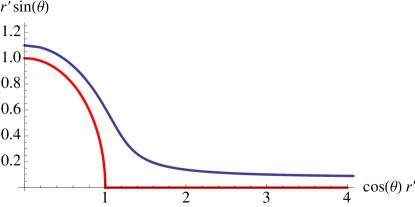
Figure 1: Depiction of zero mass embedding with a finite mass embedding for $\gamma=0$.

Embeddings with non–zero mass start at infinity at some non–zero $\theta_{0}$, run roughly horizontally until deviating North, skirting the singular locus and then ending on the $\theta=\pi/2$ axis. Such trajectories show that the singular locus in the interior of the geometry acts to repel the D7–branes somewhat. However, unlike other cases where repulsion generates a condensate even for the zero mass embedding giving spontaneous chiral symmetry breaking (e.g., background magnetic field [27], see also the examples in refs. [28, 29]) the condensate at zero mass remains vanishing. We depict an example in figure 1. Very high masses give embeddings that are hardly deviated by the singular locus, their behaviour being very similar to that in ordinary AdS.

For $\gamma<0$, since the 3–sphere shrinks to zero size on the singular locus, one might think that no extension is needed, with the D7–brane ending at $r^{\prime}_{0}$ and some value of $\theta$. This would be analogous to the finite temperature case, with the singular locus playing a role similar to the horizon[28, 30, 31]. However, a study of the induced metric on the D7–brane as they approach the singular locus shows that embeddings that end on the singular locus will have a conical singularity. Therefore, for $\gamma<0$, no embeddings can end at $r=r_{0}^{\prime}$, and they must run to some final value of $r^{\prime}$ at $\theta=\pi/2$. An example of such a consistent embedding is shown in figure 2. A direct consequence of this result is that for $\gamma<0$, no zero mass embedding exists. There is in fact a minimum mass embedding, and as $\gamma$ decreases, the minimum mass increases in value. We show this in figure 3, plotting the bare mass against $-\gamma$. (Recall that $\theta_{0}=2\pi\alpha^{\prime}m_{q}/R$.) For a given non–zero $\gamma$, this “gap” in the spectrum of allowed masses is set by the adjoint mass $k=mR$.

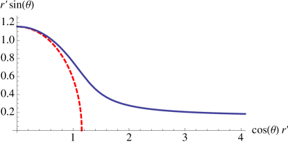
Figure 2: Depiction of lowest mass embedding for $\gamma=-0.002$. The red, dashed line is the singular locus.

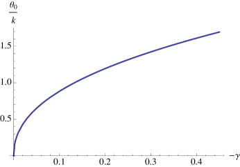
Figure 3: Lowest mass as a function of $\gamma$.

3.5 Some Analytics

Consider solving for the field $\theta(\hat{z})$ analytically as an expansion in small $k$. We proceed by defining a new field:

$$\Phi(\hat{z})=\sin(\theta(\hat{z}))=f_{0}(\hat{z})+k^{2}f_{1}(\hat{z})+\mathcal{O}(k^{4})\ .$$ (66)

Putting this into the equations of motion, and solving for each function $f_{i}(\hat{z})$, we first find the well known solution for pure AdS :

$$f_{0}(\hat{z})=\hat{z}c_{0}\ .$$ (67)

For pure AdS, $c_{0}$ is related to the bare quark mass. The function $f_{1}(\hat{z})$ has solution given by:

$$f_{1}(\hat{z})=\frac{c_{1}\hat{z}+c_{2}\hat{z}^{3}+\frac{1}{3}c_{0}\hat{z}^{3}-c_{0}^{3}\hat{z}^{5}-\frac{2}{3}c_{0}\hat{z}^{3}\ln(\hat{z})-\frac{4}{3}c_{0}^{3}\hat{z}^{5}\ln(k\hat{z})}{1-c_{0}^{2}\hat{z}^{2}}\ ,$$ (68)

where $(c_{1},c_{2})$ are constants. These constants can be chosen based on some dimensional analysis [25] to be:

$$c_{1}=-\frac{1}{3c_{0}}\ ,\quad c_{2}=-\frac{2}{3}c_{0}\ln(c_{0})\ .$$ (69)

Comparing to equation (52), we can extract the asymptotic constants to be given by:

$$\theta_{0}=c_{0}-\frac{k^{2}}{3c_{0}}\ ,\quad\theta_{2}=\frac{c_{0}^{3}}{6}+k^{2}\left(-\frac{c_{0}}{6}-\frac{2}{3}c_{0}\ln(c_{0})\right)\ .$$ (70)

Substituting this into our condensate, we find that:

$$C=0+\mathcal{O}(k^{4})\ .$$ (71)

Now, from dimensional analysis, the condensate should have the following expansion in terms of $m/m_{q}$:

$$C=m_{q}^{3}\left(o_{0}+\left(\frac{m}{m_{q}}\right)^{2}o_{1}+\left(\frac{m}{m_{q}}\right)^{4}o_{2}+\dots\right)\ ,$$ (72)

for constants $o_{i}$. Combining this with our result in equation (71) (recall $k=mR$) tells us that the large mass limit of the condensate is zero.

Another useful result to consider is how the mass and condensate scale. In particular, we note that the background only depends on the combination $k\hat{z}$, and therefore, we can absorb the constant $k$ into a new coordinate $\tilde{z}$. The asymptotic expansion for $\theta(\tilde{z})$ is given by:

$$\theta(\tilde{z})=\tilde{z}\left(\tilde{\theta}_{0}+\tilde{z}^{2}\left(\tilde{\theta}_{2}-\frac{2}{3}\tilde{\theta}_{0}\ln(\tilde{z})\right)\right)\ .$$ (73)

If we introduce the coordinate $\hat{z}$ into this expression, we find that (c.f. equation (52)):

$$\theta_{0}=k\tilde{\theta}_{0}\ ,\quad\theta_{2}=k^{3}\left(\tilde{\theta}_{2}-\frac{2}{3}\tilde{\theta}_{0}\ln(k)\right)\ .$$ (74)

Therefore, we learn that the bare quark mass should scale linearly with $k$. Substituting this result into our expression for the condensate, we find that:

$$C=k^{3}\tilde{C}=k^{3}\left(-2\tilde{\theta}_{2}+\frac{1}{3}\tilde{\theta}_{0}^{3}-\frac{4}{3}\tilde{\theta}_{0}\ln(\tilde{\theta}_{0})\right)\ .$$ (75)

The condensate should scale as $k^{3}$. These results will be very useful, as we shall see later.

3.6 Numerical Regularization

Before physics can be extracted from the numerical solution of the non–linear equations of motion that result from the actions we write, we must remove any systematic numerical effects that can occur in regimes where accuracy is compromised by cancellation among very large or very small numbers. Typically, these manifest themselves at high bare quark mass in the condensate vs. mass curve, since in that regime we are near the AdS boundary, where the conformal factor naturally grows rapidly. We know from the previous section that the condensate should fall to zero in this regime. The raw numerical results plotted in figure 4 show that this is masked by an offset. It is purely numerical and unphysical (it is very similar to the deviation from zero seen for probe D7–branes in pure AdS in global coordinates [25]), and may be consistently subtracted from all subsequent computations. The deviation from zero occurs for all values of $k$, and therefore, in order to isolate the purely numerical piece to use as a regulator, we choose to subtract off the curve for small $k$ (here we use $k=10^{-1}$). After the appropriate rescaling given in equation (75), this curve can be used to extract the physical condensate at higher $k$. We stress again that this subtraction is not physical in the sense that it is not akin to a contribution of an unknown counterterm. We have treated those fully in section 3.2.

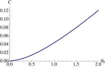
Figure 4: Raw numerical data for the condensate as a function of bare quark mass for $k^{2}=10^{-2}$. The deviation from zero for increasing mass is a numerical artifact, which we subtract in all later computations. Recall that $\theta_{0}=m_{q}\times(2\pi\alpha^{\prime}/R)$.

Using this procedure, we calculate the physical condensate in figure 5(a). It is important to test that we have not damaged the physics, and to that end we rescale each curve according to equation (75) and find they exactly match as shown in figure 5(b). We also present results for $\gamma<0$, where we see that the absence of the states below a minimum mass (see section 3.4) simply removes a piece from the condensate curve (see figure 6).

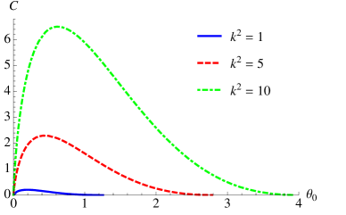
(a) Not scaled

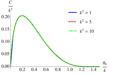
(b) Scaled

Figure 5: Condensate as a function of bare quark mass for $k^{2}=1,5,10$ for $\gamma=0$. Recall that $\theta_{0}/k=m_{q}/m\times(2\pi\alpha^{\prime}/R^{2})$.

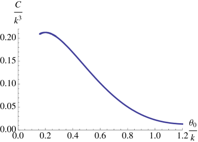
Figure 6: Condensate as a function of bare quark mass for $\gamma=-0.002$. Recall that $\theta_{0}/k=m_{q}/m\times(2\pi\alpha^{\prime}/R^{2})$.

4 Constituent Quark Mass

An important quantity to compute is the constituent quark mass. This is given by the energy of a fundamental string stretching from the D7–brane to the core of the geometry (made of D3–branes), starting at the place the D7–brane ends. This is to be contrasted with the bare quark mass, which is the asymptotic separation of the D7–brane from the D3–branes, extracted in the UV. The two types of mass are readily visualized on figures 1 and 2. Far to the right the vertical distance from embedding to the horizontal axis gives the bare quark mass. Far to the left, on the $\theta=\pi/2$ axis, the vertical distance from where the embedding ends to the singular locus gives the constituent quark mass.

For the constituent quark mass, we calculate the energy of a string that hangs from the point where the $S^{3}$ has shrunk to zero size (let us denote this point as $z_{m}$) to $z=\infty$. In order to do this, we consider the Nambu–Goto action for the fundamental string (in Einstein frame) given by:

$$S=\frac{1}{2\pi\alpha^{\prime}}\int d^{2}\sigma e^{\Phi/2}\sqrt{-h}=\frac{1}{2\pi\alpha^{\prime}}\int d^{2}\sigma\mathcal{L}\ .$$ (76)

Working in static gauge, we take as coordinates for the string worldsheet $\sigma^{0}=t$ and $\sigma^{1}=z$. In these coordinates, the string does not couple to the NS–NS 2–form potential of the background. The physical energy (the constituent quark mass) is then given by the action (per unit time) multiplied by a factor of two to remove the factor of 1/2 from $g_{tt}$ near the AdS boundary):

$$\frac{2\pi\alpha^{\prime}}{R}m_{c}=2k\int_{z_{m}}^{\infty}dz\frac{\rho^{4}\coth(2\chi)}{z}\ .$$ (77)

It is convenient to use $\chi$ as an integration variable to write (with the help of equations (10) and (12)) this equation as:

$$\frac{2\pi\alpha^{\prime}}{R}m_{c}=4k\int_{\chi_{m}}^{\infty}d\chi\ \mathrm{csch}(2\chi)\coth(2\chi)=2k\ \mathrm{csch}(2\chi_{m})\ .$$ (78)

We present the results for this in figure 7, for the case $\gamma=0$. The key result here is that the constituent mass is always greater than the bare quark mass, and it is significantly greater as the D7–brane approaches the singular locus. This result suggests that the embeddings experience a repulsive force from the background, as we observed earlier.

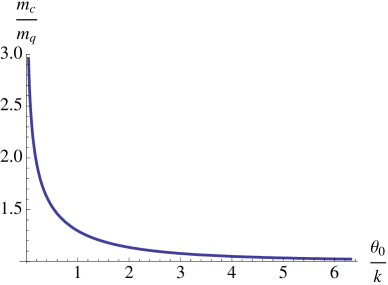
Figure 7: Constituent to bare quark mass ratio vs. bare mass to adjoint mass ratio for the case $\gamma=0$. Recall that $\theta_{0}/k=m_{q}/m\times(2\pi\alpha^{\prime}/R^{2})$.

5 Meson Spectrum

We proceed to calculate part of the meson spectrum by calculating the quadratic fluctuations associated with the field $\theta(z)$ [21]:

$$\theta(z)=\theta_{0}(z)+2\pi\alpha^{\prime}\Phi(t,z)\ ,$$ (79)

where $\theta_{0}(z)$ is the solution we found in the previous section. Substituting this form into the Lagrangian and keeping only terms quadratic in $\Phi$, we can calculate the equations of motion for the field $\Phi(t,z)$. Assuming a time dependence of the form:

$$\Phi(t,z)=e^{-i\omega t}\phi(z)\ ,$$ (80)

the asymptotic form $g_{tt}\to\frac{R^{2}}{2z^{2}}$ means that $\omega$ is related to the mass of the meson via:

$$M=2\omega\ .$$ (81)

Following a similar scaling analysis to that done in section 3.5, we find that $\omega$ scales linearly with $k$, and therefore the relevant quantity for us will be the ratio of the two. We plot our results for the spectrum (extracted using fairly standard techniques presented for example in ref.[32]) in figure 8. As the figure indicates, the spectrum approaches that of pure AdS as the bare quark mass increases. Furthermore, the mass of the meson is consistently above that of pure AdS, which is consistent with our previous result that the D7–brane feels a repulsive force. Finally, we find that the behavior of the curve near zero mass is well approximated by a function of the following form:

$$\frac{2R}{k}\omega=a\left(\frac{\theta_{0}}{k}\right)^{1/2}+b\frac{\theta_{0}}{k}\ ,$$ (82)

where $(a,b)$ are constants. This is reminiscent of the form of the GMOR relation [33], although there is no spontaneous chiral symmetry breaking here. It is worth exploring further the origin of this behaviour, including how strongly it depends upon us having restricted to $\phi=(2n+1)\pi/2$.

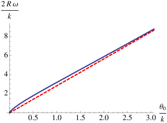
(a) Meson Spectrum

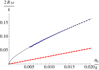
(b) Meson Spectrum Near Origin

Figure 8: Lowest level of the meson spectrum as a function of bare quark mass. (Recall that $\theta_{0}/k=m_{q}/m\times(2\pi\alpha^{\prime}/R^{2})$.) The red–dashed line corresponds to the lowest level of the spectrum for $k=0$, i.e. pure AdS${}_{5}\times S^{5}$ studied in ref. [32]. In the figure to the right, the black line corresponds to the best fit curve.

We consider separately the calculation of the meson spectrum for our zero mass embedding. We only need to consider the fluctuations of the $\theta=0$ embedding to extract this. Following the same procedure as before (but now in terms of the coordinate $r^{\prime}$), we find near the singular locus the solution for the fluctuation goes as:

$$\phi(r^{\prime})\propto(r^{\prime}-1)^{-2}e^{\frac{\pm 3i\hat{\omega}}{2(r^{\prime}/R-1)}}\ ,$$ (83)

where $\hat{\omega}=R\omega/k$. This behavior is exactly the ingoing/outgoing wave behavior we would expect for fluctuations near the event horizon of an extremal black hole [32]. Since we want our field to satisfy ingoing wave boundary conditions (the plus sign), we can define a new field:

$$\phi(r^{\prime})=(r^{\prime}-1)^{-2}e^{\frac{3i\hat{\omega}}{2(r^{\prime}/R-1)}}y(r^{\prime})\ .$$ (84)

Near the AdS boundary, $y(r^{\prime})$ behaves as:

$$y(r^{\prime})\to c_{1}r^{\prime}+\frac{c_{2}}{r^{\prime}}\ ,$$ (85)

and we require that $c_{1}=0$ such that we only have a normalizable mode. We find that for a starting position of $r^{\prime}=1+\epsilon$, the value of $\hat{\omega}$ that satisfies the normalizibility condition is given by $\hat{\omega}\approx-i\epsilon 7.7\times 10^{-4}$ (starting with $\epsilon=10^{-3})$. Sending $\epsilon$ to zero gives us $\hat{\omega}=0$, which means we have a (stable) zero mass meson for zero bare quark mass.

6 Conclusions

The results for our D7–brane probe analysis fit nicely with what had already been established for this background using D3–brane probes [15, 16]. The enhançon locus, the special place the D3–branes become massless, is also the place where the D7–branes that are massless quark flavours end. All other D7–branes end above that locus, and in fact are somewhat bent away from it in their profile.

It this way we have confirmed the prediction of ref. [29] that there is no chiral symmetry breaking in this background (although they seem to have thought that this form of the embedding would depend on one of the angles of the $S^{3}$, which we show is not necessary), since the zero mass embedding is not repelled by the enhançon (hence no chiral condensate). The higher mass embeddings do have a condensate associated with them of course, and we have explored the dependence on mass, finding it to be smooth, regardless of the value of the adjoint mass. Much the same can be said about the accompanying spectrum of mesons we explored.

We have not addressed the meaning of our particular choices for the value of $\phi$, which allowed us to find the solutions. $\phi$ is related to the phase angle of the mass matrix in the dual theory [34], and so it seems that this particular choice may have some physical meaning, but we have not yet explored that.

An important question to address is whether these choices are stable under fluctuations. Unfortunately, due to the complicated nature of the $C_{(6)}$ and $C_{(8)}$, we are not able to address this question by considering fluctuations of the field $\phi$ around our special values. However, it is important to note that the massless embedding is special here. The $\phi$–dependence simplifies even further at $\theta=0$, vanishing entirely. This suggests that the zero mass embedding persists for any value of $\phi$, as might have been expected, and that there are additional symmetries in that case. Possibly the embedding itself is supersymmetric, but in addition there is probably a continuous symmetry (translations in $\phi$) that appears for that sector. This may also be connected to the GMOR–like behaviour that we observed for the meson mass dependence as the bare quark mass approaches zero, although that meson is from the $\theta$ fluctuations, and we do not have a spontaneous symmetry breaking here.

There appears to be some qualitative similarities between features of our solution and that of solutions in global AdS. It seems that our parameter $k=mR$, the adjoint mass, plays a similar role to the inverse radius of the $S^{3}$ on which the dual theory lives. A similar modification to the asymptotics in the field $\theta$ occurs, so we find a similar counterterm is needed. It would be nice to understand this further. The type of counterterms that can arise seem connected to the way in which the (non-thermal) parameter/deformation under discussion is introduced. Sometimes it is at the level of the background itself (such as in the global case, of the case here) while in the case of a finite magnetic field [27] or chemical potential [25] where there is no logarithmic behavior, the parameter is introduced at the level at the level of the D7–brane action itself. This is worth further exploration.

References

- [1] J. M. Maldacena, “The large n limit of superconformal field theories and supergravity,” Adv. Theor. Math. Phys. 2 (1998) 231–252, hep-th/9711200.
- [2] E. Witten, “Anti-de sitter space and holography,” Adv. Theor. Math. Phys. 2 (1998) 253–291, hep-th/9802150.
- [3] S. S. Gubser, I. R. Klebanov, and A. M. Polyakov, “Gauge theory correlators from non-critical string theory,” Phys. Lett. B428 (1998) 105–114, hep-th/9802109.
- [4] C. V. Johnson, “D-branes,”. Cambridge, USA: Univ. Pr. (2003) 548 p.
- [5] The ALICE Collaboration, K. Aamodt et al., “Elliptic flow of charged particles in Pb-Pb collisions at 2.76 TeV,” arXiv:1011.3914 [nucl-ex].
- [6] C. V. Johnson and P. Steinberg, “What black holes teach about strongly coupled particles,” Phys. Today 63N5 (2010) 29–33.
- [7] B. Jacak and P. Steinberg, “Creating the perfect liquid in heavy-ion collisions,” Phys. Today 63N5 (2010) 39–43.
- [8] J. E. Thomas, “The nearly perfect Fermi gas,” Phys. Today 63N5 (2010) 34–37.
- [9] J. Casalderrey-Solana, H. Liu, D. Mateos, K. Rajagopal, and U. A. Wiedemann, “Gauge/String Duality, Hot QCD and Heavy Ion Collisions,” arXiv:1101.0618 [hep-th].
- [10] A. Buchel and J. T. Liu, “Thermodynamics of the N = 2* flow,” JHEP 11 (2003) 031, hep-th/0305064.
- [11] A. Buchel, “N = 2* hydrodynamics,” Nucl. Phys. B708 (2005) 451–466, hep-th/0406200.
- [12] A. Buchel, S. Deakin, P. Kerner, and J. T. Liu, “Thermodynamics of the N = 2* strongly coupled plasma,” Nucl. Phys. B784 (2007) 72–102, arXiv:hep-th/0701142.
- [13] A. Buchel and C. Pagnutti, “Bulk viscosity of N=2* plasma,” Nucl. Phys. B816 (2009) 62–72, arXiv:0812.3623 [hep-th].
- [14] K. Pilch and N. P. Warner, “N = 2 supersymmetric RG flows and the IIB dilaton,” Nucl. Phys. B594 (2001) 209–228, hep-th/0004063.
- [15] A. Buchel, A. W. Peet, and J. Polchinski, “Gauge dual and noncommutative extension of an N = 2 supergravity solution,” Phys. Rev. D63 (2001) 044009, hep-th/0008076.
- [16] N. J. Evans, C. V. Johnson, and M. Petrini, “The enhancon and N = 2 gauge theory/gravity RG flows,” JHEP 10 (2000) 022, arXiv:hep-th/0008081.
- [17] C. V. Johnson, A. W. Peet, and J. Polchinski, “Gauge theory and the excision of repulson singularities,” Phys. Rev. D61 (2000) 086001, hep-th/9911161.
- [18] N. Seiberg and E. Witten, “Monopole Condensation, And Confinement In N=2 Supersymmetric Yang-Mills Theory,” Nucl. Phys. B426 (1994) 19–52, arXiv:hep-th/9407087.
- [19] N. Seiberg and E. Witten, “Monopoles, duality and chiral symmetry breaking in N=2 supersymmetric QCD,” Nucl. Phys. B431 (1994) 484–550, arXiv:hep-th/9408099.
- [20] A. Karch and E. Katz, “Adding flavor to ads/cft,” JHEP 06 (2002) 043, hep-th/0205236.
- [21] A. Karch, E. Katz, and N. Weiner, “Hadron masses and screening from ads wilson loops,” Phys. Rev. Lett. 90 (2003) 091601, hep-th/0211107.
- [22] S. S. Gubser, “Curvature singularities: The good, the bad, and the naked,” Adv. Theor. Math. Phys. 4 (2000) 679–745, arXiv:hep-th/0002160.
- [23] S. Kobayashi, D. Mateos, S. Matsuura, R. C. Myers, and R. M. Thomson, “Holographic phase transitions at finite baryon density,” JHEP 02 (2007) 016, hep-th/0611099.
- [24] A. Karch, A. O’Bannon, and K. Skenderis, “Holographic renormalization of probe d-branes in ads/cft,” JHEP 04 (2006) 015, hep-th/0512125.
- [25] A. Karch and A. O’Bannon, “Chiral transition of N=4 super Yang-Mills with flavor on a 3-sphere,” Phys.Rev. D74 (2006) 085033, arXiv:hep-th/0605120 [hep-th].
- [26] C. Hoyos, “Higher dimensional conformal field theories in the Coulomb branch,” Phys. Lett. B696 (2011) 145–150, arXiv:1010.4438 [hep-th].
- [27] V. G. Filev, C. V. Johnson, R. C. Rashkov, and K. S. Viswanathan, “Flavoured large N gauge theory in an external magnetic field,” JHEP 10 (2007) 019, arXiv:hep-th/0701001.
- [28] J. Babington, J. Erdmenger, N. J. Evans, Z. Guralnik, and I. Kirsch, “Chiral symmetry breaking and pions in non-supersymmetric gauge / gravity duals,” Phys. Rev. D69 (2004) 066007, hep-th/0306018.
- [29] N. Evans, J. Shock, and T. Waterson, “D7 brane embeddings and chiral symmetry breaking,” JHEP 03 (2005) 005, hep-th/0502091.
- [30] T. Albash, V. G. Filev, C. V. Johnson, and A. Kundu, “A topology-changing phase transition and the dynamics of flavour,” Phys. Rev. D77 (2008) 066004, arXiv:hep-th/0605088.
- [31] D. Mateos, R. C. Myers, and R. M. Thomson, “Holographic phase transitions with fundamental matter,” Phys. Rev. Lett. 97 (2006) 091601, arXiv:hep-th/0605046.
- [32] M. Kruczenski, D. Mateos, R. C. Myers, and D. J. Winters, “Meson spectroscopy in ads/cft with flavour,” JHEP 07 (2003) 049, hep-th/0304032.
- [33] M. Gell-Mann, R. J. Oakes, and B. Renner, “Behavior of current divergences under su(3) x su(3),” Phys. Rev. 175 (1968) 2195–2199.
- [34] T. Albash, V. G. Filev, C. V. Johnson, and A. Kundu, “Global Currents, Phase Transitions, and Chiral Symmetry Breaking in Large N(c) Gauge Theory,” JHEP 12 (2008) 033, arXiv:hep-th/0605175.