Objectively discerning Autler-Townes Splitting
from Electromagnetically Induced Transparency

Abstract

Autler-Townes splitting (ATS) and electromagnetically-induced transparency (EIT) both yield transparency in an absorption profile, but only EIT yields strong transparency for a weak pump field due to Fano interference. Empirically discriminating EIT from ATS is important but so far has been subjective. We introduce an objective method, based on Akaike’s information criterion, to test ATS vs. EIT from experimental data and determine which pertains. We apply our method to a recently reported induced-transparency experiment in superconducting circuit quantum electrodynamics.

Coherent processes in atoms and molecules yield many interesting and practical phenomena such as coherent population trapping Arimondo (1996), lasing without inversion Kocharovskaya (1992), and electromagnetically induced transparency (EIT) Marangos (1998). Pioneering EIT experiments employed alkali metals due to their simple electronic level structure and long-lived coherence, but recently coherent processes are investigated in other systems such as quantum dots Xu et al. (2008), nanoplasmonics Liu et al. (2009), superconducting circuits Kelly et al. (2010), metamaterials Papasimakis et al. (2008); Zhang et al. (2008), and optomechanics Safavi-Naeini et al. (2011). EIT is also observed for classical coupled oscillator, e.g. inductively or capacitively coupled electrical resonator circuits Lamb and Retherford (1951); Alzar et al. (2002). EIT systems could enable new practical applications of coherent processes, but the lack of time-scale separations characteristic of alkalis Fleischhauer et al. (2005) obfuscates signatures of coherent processes.

Here we focus on EIT, where transparency is induced coherently by a pump field even if the pump is arbitrarily weak. EIT is crucial for optically-controlled slowing of light Hau et al. (1999) and optical storage Phillips et al. (2001) and is achieved by Fano interference Fano (1961) between two atomic transitions. Without Fano interference, EIT is simply Autler-Townes splitting (ATS), equivalently the ac-Stark effect Autler and Townes (1955), corresponding to a doublet structure in the atomic-absorption profile that requires strong pumping. In essence, both EIT and ATS lead to the presence of a transparency window due to electromagnetic (EM) pumping, but the mechanisms are entirely different. Here we introduce an objective test for use on empirical data to discern EIT from ATS in any experiment. This test is based on Akaike weights for the models Burnham and Anderson (2002) and reveals whether EIT or ATS has been observed or whether the operating conditions make the data inconclusive.

Fano’s seminal study of two nearly-resonant modes decaying via a common channel differed from the prevalent normal-mode analyses at the time: he showed that this shared decay channel yields additional cross-coupling between modes mediated by the common reservoir, which explained the anomalous asymmetric lineshape for electrons scattering from Helium Fano (1961). In fact any response that combines multiple modes can have Fano interference, which can be extremely sharp and highly sensitive to variability in the system Hao et al. (2008).

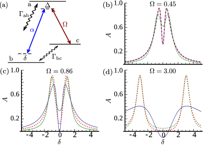
Harris and Imamoğlu showed that hybrid “atom+field” modes in the dressed-state formalism interact with the same reservoir hence readily satisfy the Fano interference conditions Imamoğlu and Harris (1989) thereby producing a transparency window in the absorption profile $A(\delta)$ for $\delta$ the two-photon detuning frequency. This effect was originally demonstrated for a $\Lambda$-type three-level atom (TLA) with energy levels $|a\rangle$, $|b\rangle$, and $|c\rangle$ and judiciously chosen rates as shown in Fig. 1(a). Dressed-state frequency separation is proportional to the pump-field Rabi frequency $\Omega$, and this separation yields ATS in the absence of Fano interference. Fano interference is negligible for large $\Omega$ but must transition smoothly from ATS to EIT as $\Omega$ decreases and the dressed states try to merge thereby strengthening the Fano interference effect. Under EIT conditions, complete transparency holds even in the weak-pump limit.

Figure 1: (Color online) (a) $\Lambda$-type TLA with probe (pump) driving field with Rabi frequency $\alpha$ ($\Omega$), which probes (drives) the $|a\rangle\leftrightarrow|b\rangle$ ($|a\rangle\leftrightarrow|c\rangle$) transition. (b-d) Absorption $A$ vs. two-photon detuning $\delta$ (red dots) for resonant ($\Delta=0$) pump with $\Gamma_{\text{ab}}=1$, $\Gamma_{\text{bc}}=0.1$ and various $\Omega$ with best fits to $A_{\text{EIT}}(C_{+},C_{-},\gamma_{+},\gamma_{-})$ (blue solid) and $A_{\text{ATS}}(C,\gamma,\delta_{0})$ (green dashed) models calculated for (b) weak $\Omega$ with good fit to $A_{\text{EIT}}(2.14,1.89,0.581,0.520)$ and poor fit to closest $A_{\text{ATS}}(0.532,0.633,0.712)$, (c) intermediate $\Omega$ with poor fit to closest $A_{\text{ATS}}(0.472,0.512,1.03)$ as well as $A_{\text{EIT}}(88.3,88.3,0.75,0.752)$, and (d) strong $\Omega$ with poor fit to closest $A_{\text{EIT}}(1.3\times 10^{3},1.3\times 10^{3},2.92,2.92)$ and good fit to $A_{\text{ATS}}(0.499,0.521,3.05)$.

There are four TLAs: $\Lambda$, V, and two ladder ($\Xi$) cascade systems with upper- and lower-level driving, respectively. Only $\Lambda$- and upper-level-driven $\Xi$ TLAs exhibit Fano interference-induced suppression of absorption Lee et al. (2000). For simplicity, we focus on the $\Lambda$ TLA to show how the decaying dressed-states formalism yields distinctive absorption profiles characteristic of EIT and ATS Anisimov and Kocharovskaya (2008); Abi-Salloum (2010), but our approach to discern EIT from ATS is independent of the choice of TLA so directly applicable to upper-level-driven $\Xi$-type TLA.

We use a semiclassical description with decay and dephasing rates manually inserted. The EM response to the probe is proportional to the probe-induced excited coherence corresponding to the off-diagonal TLA density matrix element $\sigma_{\text{ab}}$. The steady-state solution to linear order of the probe electric field has all population in $|b\rangle$ so excited coherence at the probed transition depends only on dephasing rates $\Gamma_{\text{ab}}$ and $\Gamma_{\text{bc}}$: $\sigma_{\text{ab}}=\alpha/[\delta+\Delta-\text{i}\Gamma_{\text{ab}}-\Omega^{2}/(\delta-\text{i}\Gamma_{\text{bc}})]$, with $\Delta$ the one-photon detuning and $\alpha$ the probe Rabi frequency Anisimov and Kocharovskaya (2008).

Linear absorption $A\propto\text{Im}(\sigma_{\text{ab}})$, shown in Figs. 1(b-d), has spectral poles $\delta_{\pm}=-\Delta/2+\text{i}(\Gamma_{\text{ab}}+\Gamma_{\text{bc}})/2\pm[\Omega^{2}+(\Delta-\text{i}\Gamma_{\text{ab}}+\text{i}\Gamma_{\text{bc}})^{2}/4]^{1/2}$, which produce resonant contributions to atomic response, $A_{\pm}=S_{\pm}/(\delta-\delta_{\pm})$, with strengths $S_{\pm}=\pm(\delta_{\pm}-\text{i}\Gamma_{\text{bc}})/(\delta_{+}-\delta_{-})$. These resonant contributions can be attributed to “decaying-dressed states” Anisimov and Kocharovskaya (2008) with frequencies and dephasing rates given by Re$(\delta_{\pm})$ and Im$(\delta_{\pm})$, respectively. Decaying-dressed states arise from the interaction between dressed states with eigenenergies $-\Delta/2\pm(\Omega^{2}+\Delta^{2}/4)^{1/2}$ and two reservoirs with decay rates $\Gamma_{\text{ab}}$ and $\Gamma_{\text{bc}}$. This interaction is affected by the pump in two ways: separating dressed-states and exciting the $|a\rangle\leftrightarrow|c\rangle$ transition needed for destructive Fano interference with the $|a\rangle\leftrightarrow|b\rangle$ reservoir. Unfortunately, the excited $|a\rangle\leftrightarrow|c\rangle$ transition interacts with the $|b\rangle\leftrightarrow|c\rangle$ reservoir, which is always positive and thus negates absorption suppression. Finally, one-photon detuning further separates dressed states thereby weakening Fano interference.

Strong Fano interference, hence strong EIT, occurs for resonant driving ($\Delta=0$) where the spectral poles exist in three $\Omega$-regions: (i) dressed states share a reservoir $\Omega\leq\Omega_{\text{EIT}}\equiv\left(\Gamma_{\text{ab}}-\Gamma_{\text{bc}}\right)/2$, (ii) dressed states decay into distinct reservoirs $\Omega\gg\Gamma_{\text{ab}}$, and (iii) intermediate regime where the dressed-state reservoirs are only partially distinct. In $\Omega$-region (i) $\text{Re}(\delta_{\pm})=0=\text{Im}(S_{\pm})$ so the absorption profile comprises two Lorentzians centered at the origin, one broad and positive and the other narrow and negative: $A_{\text{EIT}}=C^{2}_{+}/(\gamma_{+}^{2}+\delta^{2})-C^{2}_{-}/(\gamma_{-}^{2}+\delta^{2})$. Hence, low-power pump-induced transparency, where Fano interference dominates, has a transparency window without splitting Anisimov and Kocharovskaya (2008). For strong-pump $\Omega$-region (ii) $\delta_{\pm}\approx\pm\Omega+\text{i}(\Gamma_{\text{ab}}+\Gamma_{\text{bc}})/2$ and $S_{\pm}\approx 1/2$ so $A_{\text{ATS}}=C^{2}[1/(\gamma^{2}+\left(\delta-\delta_{0}\right)^{2})+1/(\gamma^{2}+\left(\delta+\delta_{0}\right)^{2})]$, corresponding to the sum of two equal-width Lorentzians shifted from the origin by $\delta_{0}\approx\pm\Omega$.

Figures 1(b-d) demonstrate how well these EIT and ATS models fit calculated absorption profiles, but an objective criterion is needed to discern the best model or whether the data are inconclusive. Akaike’s Information Criterion (AIC) identifies the most informative model based on Kullback-Leibler divergence (relative entropy), which is the average logarithmic difference between two distributions with respect to the first distribution. AIC quantifies the information lost when model $A_{i}$ with $K_{i}$ fitting parameters is used to fit actual data: $I_{i}=-2\log\mathcal{L}_{i}+2K_{i}$ for $\mathcal{L}_{i}$ the maximum likelihood for model $A_{i}$ with penalty $2K_{i}$ for fitting parameters Burnham and Anderson (2002).

Figure 2: (Color online) (a) Akaike weights vs. Rabi frequency for the TLA in Fig. 1 showing a sharp transition at $\Omega_{\text{AIC}}$ from EIT model (blue solid) to ATS model (green dashed); (b) Transition boundary $\Omega_{\text{AIC}}$ with corresponding transparency values vs. $\Gamma_{\text{bc}}$.

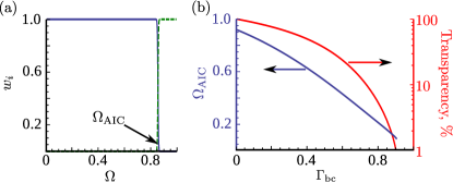
We demonstrate AIC-based testing by fitting an absorption data set $D=\{A(\delta_{j});|\delta_{j}|\leq 5\}$, incrementing in steps $\Delta\delta_{j}=0.05$, for the TLA in Fig. 1(a) to models $A_{\text{EIT}}$ and $A_{\text{ATS}}$ using the NonlinearModelFit function in Mathematica™, which can calculate AIC. The relative likelihood of model $A_{i}$ out of $n$ models is its Akaike weight $w_{i}=\text{e}^{-I_{i}/2}/\sum_{k=1}^{n}\text{e}^{-I_{k}/2}$ depicted in Fig. 2(a). This figure shows that, based on AIC, the EIT model explains data with 100% likelihood for all $\Omega<\Omega_{\rm AIC}=0.86$. Figure 2(b) shows that increasing $\Gamma_{\text{bc}}$ reduces the EIT threshold $\Omega_{\text{AIC}}$ and guides devising EIT experiments.

Testing for EIT is affected by the fact that experiments have additional complexities such as one-photon detuning or more than three energy levels, but these complexities do not negate the validity of our test; rather these complications just make it harder to pass the EIT test. Consequently, one can construct and test more general models that accommodate these extra features because AIC allows relative testing between any number of models. The corresponding signatures of Fano interference in generalized models can be identified thus revealing genuine EIT effects.

A more important issue of working with experimental data sets $D=\{A(\delta_{j})\}$ is that experiments are noisy so each run produces a different data set, say $D_{\ell}$, with many data points measured. In turn, the Akaike weight reveals the likelihood of describing a data set $D_{\ell}$ that becomes binary (0 or 1), hence conclusive, for large data sets as shown in Fig. 2(a). Consequently, one will conclusively say after each run which model pertains, but, because of noise, this conclusion could vary from run to run. Intuitively the best model should be picked more often, however, experimental data are not reported on per run basis. Experimental data are typically reported as mean values with error bars representing the confidence interval for the data. Hence we need to adapt the AIC based testing to the way experimental data are reported.

Akaike’s information according to the least-squares analysis is $I=N\log(\hat{\sigma}^{2})+2K$ for $\hat{\sigma}^{2}=\sum_{j=1}^{N}\hat{\epsilon}_{j}^{2}/N$ and $\hat{\epsilon}^{2}_{j}$ the estimated residuals from the fitted model Burnham and Anderson (2002). Technical noise, however, blurs the distinction between models $\{A_{i}\}$ causing Akaike’s information to become $I=N\log(\hat{\sigma}^{2}+\hat{\sigma}^{2}_{\text{exp}})+2K$ with aforementioned consequences. Hence, we propose a fitness test for Akaike’s information obtained from reported experimental data.

Our fitness test uses a per-point (mean) AIC contribution $\bar{I}=I/N$ to calculate a per-point weight for the $i^{\rm th}$ model: $\bar{w}_{i}=\exp(-\bar{I}_{i}/2)/\sum_{k=1}^{n}\exp(-\bar{I}_{k}/2)$. These unnormalized per-point weights $\exp(-\bar{I}_{i}/2)$ converge to $1/\sqrt{\hat{\sigma}^{2}_{i}}$ for large data sets; in case of noisy data, this yields equal per-point weights for all models as expected intuitively.

Figure 3: (Color online) (a) Per-point weights $\bar{w}_{i}$ for the conditions of Fig. 1 as a function of pump-field Rabi frequency $\Omega$ illustrate three distinct regions: $\Omega<\Omega_{\text{EIT}}=0.45$, where the EIT model (blue) dominates unconditionally; $0.45<\Omega<0.86$, where the ATS model (green) shows non-zero likelihood; $\Omega>0.86$, ATS model dominates. The presence of Gaussian noise with standard derivation $\sigma=0.1$ (red dots) [$\sigma=0.01$ (burgundy dots)] affects the per-point weights for EIT and ATS models leading to the absence of unconditional dominance by the EIT model. (b) In the weak-pump limit and a poor signal-to-noise ratio, both models are equally likely to fit data (red dots).

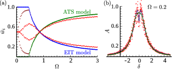
We simulate a noisy absorption profile by generating data $D_{\ell}$ according to $\left\langle A(\delta_{j})\right\rangle=(1+\xi)A(\delta_{j})$ for $\xi$ randomly chosen from the normal distribution $\exp\left[-x^{2}/2\sigma^{2}\right]/\sqrt{2\pi}\sigma$. Figure 3(a) shows our per-point weights for generated data with no noise, small noise and moderate noise for the conditions of Fig. 1. In no noise case and $\Omega<\Omega_{\text{EIT}}=0.45$, the ATS model fails and has per-point weight: $\bar{w}_{2}=0$; beyond the EIT threshold $\Omega_{\text{EIT}}$, the per-point weight for ATS starts to increases with both models describing the absorption profile equally well at $\Omega_{\rm AIC}=0.86$. This agrees with intuition about fitting models, especially a continuous trade-off between models in the intermediate regime. It is also intuitive to expect that under noisy conditions and weak pump, $\Omega^{2}<\Omega^{2}_{\sigma}=2\sigma\Gamma_{\text{ab}}\Gamma_{\text{bc}}/(1-2\sigma)$, induced transparency is buried in noise, $1-\text{Im}[\sigma_{\text{ab}}(\delta=0,\Omega)]/\text{Im}[\sigma_{\text{ab}}(\delta=0,\Omega=0)]<2\sigma$, and both models account for the absorption profile equally well [see Fig. 3(b)]. Consequently, at $\Omega=0$ and any amount of noise, per-point weights are equal to 0.5 and results are inconclusive. Increasing the pump field, however, favors the EIT model until it gives way to ATS dominance for pump strength greater than $\Omega_{\rm AIC}$. Therefore, a convincing EIT demonstration requires suppression of technical noise to the point that our per-point weights become well separated.

We apply our theory to the recent observation of induced transmission (i.e. transparency), reported as EIT, for an open transmission line of a superconducting circuit with a single flux-type artificial atom (‘flux qubit’) Abdumalikov et al. (2010). In contrast to TLA system discussed here, a flux qubit driven/probed by microwave fields, which are polarized and confined to one dimension, presents a nearly lossless upper-pumped $\Xi$ system. Nevertheless, EIT testing of this observation is straightforward, with absorption being effectively replaced by reflection, since their analysis shows that transmission coefficient agrees with the electromagnetic response for a TLA: $t=1-(\gamma_{\text{ab}}/2)/[\Gamma_{\text{ab}}+i\delta+\Omega^{2}/(\Gamma_{\text{bc}}+i\delta)]$ with our Rabi frequency $\Omega$ being half their Rabi frequency Abdumalikov et al. (2010).

Induced transparency is evident from calculating Re$(t)$ for the probe field in the presence of the control field. Their system has population relaxation rate $\gamma_{\text{ab}}/2\pi=11$ MHz and dephasing rates $\Gamma_{\text{ab}}/2\pi=7.2$ MHz and $\Gamma_{\text{bc}}=0.96\Gamma_{\text{ab}}$. Therefore, the transparency window appears for a control field amplitude of $\Omega/2\pi=6$ MHz, which exceeds $\Omega_{\text{EIT}}/2\pi=0.15$ MHz so the experiment operates in a region where demonstrating Fano interference must be inconclusive.

Figure 4: (Color online) Transmission Re$(t)$ vs. two-photon detuning $\delta$ for (a) theoretical curve (red dots) with parameters taken from Ref. Abdumalikov et al. (2010) and control-field amplitude $\Omega=6$ MHz compared to the best-fit $A_{\text{EIT}}(25.4,24.2,6.36,6.15)$ (blue solid) and $A_{\text{ATS}}(4.42,7.1,6.1)$ (green dashes) and (b) actual experimental data form Ref. Abdumalikov et al. (2010) (red dots) vs. best-fit $A_{\text{EIT}}(11.8,9.08,6.77,5.66)$ (blue solid) and $A_{\text{ATS}}(4.59,7.29,5.49)$.

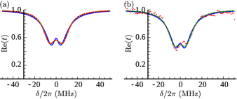
In fact the theoretical transmission curve based on the reported parameters, shown in Fig. 4(a), is indistinguishable from the best-fit ATS model and clearly distinct from the EIT model. This is further corroborated by our per-point weight that yields $\bar{w}_{1}=0.03$ implying that the result is far from EIT. Whereas the reported induced transparency suffices for switching of propagating waves in a superconducting circuit Abdumalikov et al. (2010), our objective test shows conclusively that they demonstrated ATS and definitely not EIT.

Due to noise, however, the actual experimental data shown in Fig. 4(b) differs from the theoretical prediction discussed above and shown in Fig. 4(a) so a reported data set does not conclusively show EIT nor rule it out. That is, optimal choices of $A_{\text{EIT}}$ and $A_{\text{ATS}}$ seem to fit the data equally well. Yet, there is a slight preference for ATS according to our per-point weight criterion, $\bar{w}_{1}=0.48$ and $\bar{w}_{2}=0.52$, in the weak-field limit with obvious favoring of ATS in the strong-field regime.

In conclusion, we propose an objective way to discern ATS vs. EIT from experimental data obtained in systems that demonstrate a smooth transition from ATS to EIT through three qualitative regions as the strength of the driving field $\Omega$ decreases. The Akaike weight provides a rigorous criterion to ascertain from each data set which of EIT or ATS pertains. We have introduced a per-point weight that accommodates experimental noise and readily produces a conclusion of whether EIT or ATS pertain as well as alternative in case that the experiment is inconclusive. In essence, our test seeks direct evidence of Fano interference, which is manifested as a negative Lorentzian in the absorption spectrum accompanied by the absence of splitting, that ATS lacks. Akaike’s information criterion, combined with our per-point weights, allows for testing arbitrarily many models simultaneously. Thus the data can be tested against a more complicated model, that takes care of additional levels, one-photon detunings as well as inhomogeneous broadenings, with greater likelihood of a conclusive result even in the presence of noise, and we have made clear that the sought-after EIT signature is Fano interference, which should appear as narrow negative Lorentzians in the data.

Our test of EIT vs. ATS is especially important if operation in the weak-pump regime is necessary for applications such as sensing so that the data unambiguously reveal whether the requisite conditions have been met. Nowadays EIT is becoming demonstrated in a multitude of experimental systems, and a proper test is needed, which can be employed for any EIT-type experiment. We have provided such a test.