The effect of phase mismatch on second harmonic generation in negative index materials

Abstract

Second harmonic generation in negative index metamaterials is considered. Theoretical analysis of the corresponding model demonstrated significant difference of this phenomenon in conventional and negative index materials. In contrast to conceptional materials there is nonzero critical phase mismatch. The behavior of interacting weaves is dramatically different when phase mismatch is smaller or greater than critical value.

I Introduction

Experimental demonstration of the phenomenon of negative index of refraction first in the microwave SSS:01 and latter in the optical regime SCCYSDK:05 ; ZFPMOB:05 has stimulated growing interest in nonlinear properties of negative index materials SarShal:07 . This interest is motivated by specifics on the interaction of electromagnetic waves with negative index materials. In combination with a nonlinear response of the optical material to electromagnetic radiation, this iteration leads to a new nonlinear optical phenomena. Study of these phenomena is of considerable importance both for better understanding of fundamentals of electrodynamics of negative index materials and their applications. One of the most fundamental property of negative index material is an opposite directionality of the Poynting vector, characterizing the energy flux, to the wave vector $\vec{k}$. On the other hand, the negative index property can be realized only on particukar wavelength intervals. These two features are offering a very unusual type of multi-wave interactions, if frequencies of interacting waves correspond to frequency intervals where optical material has different signs of refractive index. Multi-wave interaction must satisfy a phase matching condition, which is possible only when all wave vectors are pointed in the same direction Shen:84 . Therefore energy fluxes of the waves with frequencies corresponding to a negative sign of refractive index will propagate in opposite direction to those with frequencies corresponding to a positive sign of refraction index.

Such effect was suggested for the first time in ASBZ:04 , which considered the particular case of three waves interaction - second harmonic generation. A solution of the equation describing second harmonic generation in the case of exact phase matching was given in PShV:06 . The feasibility of parametric amplification using three-wave interaction for compensation losses in negative index materials was studied in PSh:06 . The dynamics of interacting wave packets propagating in negative index materials in the case of second harmonic generation was considered in MGK:07 . It was shown that in contrast to a weak intensity of pump field, at high intensities a second harmonic pulse can be trapped by the pump pulse and forced to propagate in the same direction.

In this paper we investigate second harmonic generation in the presence of phase-mismatch $\Delta$. This is an important case since phase-mismatch is more relevant to realistic experimental conditions. Additionally, it introduces two types of spatial distribution of second harmonic field intensity along the sample: monotonic and periodic 1 on the coordinate. Both cases are considered in this paper. We also studied second harmonic generation near a critical phase-mismatch value, when the material becomes transparent for the pump wave.

II Basic equations

The system of equations describing three wave interactions (one dimensional case) in a $\chi^{2}$ - medium for the slowly varying envelope and phase approximation can be written in the following form report ; Shen:84 :

$$\left(\widehat{k}_{1}\frac{\partial}{\partial z}+\frac{1}{\vartheta_{1}}\frac{\partial}{\partial t}\right)A_{1}=\imath\frac{2\pi\omega_{1}^{2}\mu(\omega_{1})}{c^{2}k_{1}}P^{NL}(\omega_{1})\exp{(-\imath k_{1}z)}$$

$$\left(\widehat{k}_{2}\frac{\partial}{\partial z}+\frac{1}{\vartheta_{2}}\frac{\partial}{\partial t}\right)A_{2}=\imath\frac{2\pi\omega_{2}^{2}\mu(\omega_{2})}{c^{2}k_{2}}P^{NL}(\omega_{2})\exp{(-\imath k_{2}z)}$$ (1)

$$\left(\widehat{k}_{3}\frac{\partial}{\partial z}+\frac{1}{\vartheta_{3}}\frac{\partial}{\partial t}\right)A_{3}=\imath\frac{2\pi\omega_{3}^{2}\mu(\omega_{3})}{c^{2}k_{3}}P^{NL}(\omega_{3})\exp{(-\imath k_{3}z)}$$

where wave numbers $k_{j},~{}j=1,2$ are defined as follows $k_{j}^{2}=\left(\omega_{j}/c\right)^{2}\varepsilon(\omega_{j})\mu(\omega_{j})$ and $\widehat{k}_{j}$ is the sign of the square root of $n_{j}^{2}=\varepsilon(\omega_{j})\mu(\omega_{j})$ and

$$P^{NL}(\omega_{1})=\chi^{2}(\omega_{1};\omega_{3},-\omega_{2})A_{3}A^{*}_{2}\exp{(\imath z(k_{3}-k_{2}))}$$

$$P^{NL}(\omega_{2})=\chi^{2}(\omega_{2};\omega_{3},-\omega_{1})A_{3}A^{*}_{1}\exp{(\imath z(k_{3}-k_{1}))}$$ (2)

$$P^{NL}(\omega_{3})=\chi^{2}(\omega_{3};\omega_{1},\omega_{2})A_{1}A_{2}\exp{(\imath z(k_{1}+k_{2}))}$$

For the case of second harmonic generation Eqs. (1) take the following form:

$$\left(\widehat{k}_{\omega}\frac{\partial}{\partial z}+\frac{1}{\vartheta_{\omega}}\frac{\partial}{\partial t}\right)A_{\omega}=\imath\frac{2\pi\omega^{2}\chi^{2}(\omega)\mu(\omega)}{c^{2}k_{\omega}}A_{2\omega}A_{\omega}^{*}\exp{(-\imath\Delta kz)}$$

$$\left(\widehat{k}_{2\omega}\frac{\partial}{\partial z}+\frac{1}{\vartheta_{2\omega}}\frac{\partial}{\partial t}\right)A_{2\omega}=\imath\frac{2\pi(2\omega)^{2}\chi^{2}(2\omega)\mu(2\omega)}{c^{2}k_{2\omega}}A_{\omega}^{2}\exp{(\imath\Delta kz)}$$

where $\Delta k=2k_{\omega}-k_{2\omega}$, $A_{\omega}$ is the fundamental wave with frequency $\omega$, and a$A_{2\omega}$ is the second harmonic generated in the material. We consider the case, when the refractive index is negative at the fundamental frequency $\omega$ and is positive at the second-harmonic frequency $2\omega$. The parameter $\Delta k$ plays an important role for the spatial distribution of the electromagnetic field along the sample. In the next section we consider both cases $\Delta k=0$ and $\Delta k\neq 0$.

III Case of ideal phase matching $\Delta k=0$

We consider second harmonic generation for continuos waves in a $\chi^{2}$ medium under ideal phase matching conditions $\Delta k=0$. The length of the sample we assume to be $L$. Using the symmetry properties of the susceptibility tensor $\chi^{2}$ with respect to permutations of $\omega$ and $2\omega$ frequencies, the mathematical model of second harmonic generation can be formulated in the following way Shen:84 ; Boyd:92 :

$$\frac{dA_{\omega}}{dz}=-\imath\frac{2K\omega^{2}\mu(\omega)}{c^{2}k_{\omega}}A_{2\omega}A_{\omega}^{*}$$ (4)

$$\frac{dA_{2\omega}}{dz}=\imath\frac{4K\omega^{2}\mu(2\omega)}{c^{2}k_{2\omega}}A_{\omega}^{2},$$ (5)

$$A_{\omega}(0)=A_{\omega}^{0},~{}~{}A_{2\omega}(L)=0,$$ (6)

where $K=2\pi\chi^{2}(2\omega)/c^{2}=\pi\chi^{2}(\omega)/c^{2}$. Let us represent the complex functions $A_{\omega}$ and $A_{2\omega}$ in terms of amplitudes $e_{1,2}$ and phases $\varphi_{1,2}$

$$A_{\omega}=e_{1}\exp{(\imath\varphi_{1})}\mspace{18.0mu}A_{2\omega}=e_{2}\exp{(\imath\varphi_{2})}.$$ (7)

Substitution of Eqs. (7) into (4) and (5) , and separation of real and imaginary parts lead to the following system of equations:

$$\frac{de_{1}}{dz}=\kappa e_{1}e_{2}\sin{(\theta)},$$

$$\frac{de_{2}}{dz}=\kappa e_{1}^{2}\sin{(\theta)},$$ (8)

$$\frac{d\theta}{dz}=\kappa\left(\frac{e_{1}^{2}}{e_{2}}+2e_{2}\right)\cos{(\theta)},$$

with boundary conditions:

$$e_{1}(0)=e_{10},~{}~{}e_{2}(L)=0.$$ (9)

Here $\theta$ and $\kappa$ are defined as follows

$$\theta=\varphi_{2}-2\varphi_{1},~{}~{}\kappa=4K\omega^{2}\mu(2\omega)/c^{2}k_{2\omega},$$ (10)

From the first two equations an integral of motion follows:

$$e_{1}^{2}-e_{2}^{2}=m_{1}^{2}=const$$ (11)

This integral of motion corresponds to the modified Manley-Row relation. In case of second harmonic generation in conventional materials the Manley-Row relation is equivalent to conservation of energy ($e_{1}^{2}+e_{2}^{2}=const$). In our case, relation (11) corresponds to conservation of total flux of the energy. The second integral of motion for the system (8) reads as:

$$e_{1}^{2}e_{2}\cos{(\theta)}=m_{2}=const.$$ (12)

The integral of motion (12) is consistent with boundary conditions (9) only if $\cos{(\theta)}=0$. Taking into account that the pump wave energy decays in $z$, we conclude that the phase difference is equal to $\theta=3\pi/2$, therefore the system of equations (8) can be represented as follows:

$$\frac{de_{1}}{dz}=-\kappa e_{1}e_{2},\mspace{18.0mu}\frac{de_{2}}{dz}=-\kappa e_{1}^{2}$$ (13)

The solution of (13) has the following form

$$e_{1}(\zeta)=m_{1}/\cos{(m_{1}(\textit{l}-\zeta))}$$

$$e_{2}(\zeta)=m_{1}\tan{(m_{1}(\textit{l}-\zeta))}$$

here $\zeta=\kappa z$ and $\textit{l}=\kappa L$. The solutions (LABEL:solutions:e1:e2) unknown parameter $m_{1}$, is the value of the fundamental field at the end of the sample. This parameter can be found from the boundary condition (9). Taking into account the Manley-Row relation (11), it leads to the transcendental equation for $m_{1}$:

$$e_{10}=m_{1}/\cos(m_{1}l).$$ (15)

This equation can be solved numerically. The solution of (15) together with (LABEL:solutions:e1:e2) determines the field distribution along the sample. The dependence of intensities $e_{1}^{2}$ and $e_{2}^{2}$ on $\zeta$ is represented in Fig.1 were the intensity boundary value $e_{1}^{2}(0)$ is chosen to be $e_{10}^{2}=3.5$, here $\textit{l}=1$ and $m_{1}=1$.

Figure 1: The dependence of the intensity of fundamental wave $e_{1}^{2}$ (solid curve) and second harmonic $e_{2}^{2}$ (dashed curve) on the distance $\zeta$ with $e_{10}^{2}=3.5$

The solution of transcendental equation  (15) for $l=1$ is shown in Fig.2. This plot illustrates the dependence of the output field intensity $e_{1}(l)=m_{1}$, as a function of $e_{10}$ (the amplitude of the fundamental field pumped into the medium). As shown in Fig.2, the formal solution of equation (15) has multiple branches. However, only the lower branch presented by a solid curve has physical meaning. Upper brunches represented by dashed curves are originated from periodicity of the $\cos$ function in (15). Both $e_{1}(\zeta)$ and $e_{1}(\zeta)$ corresponding to these branches have singularities on the interval $0\leq\zeta\leq l$ which is inconsistent with conservation of energy. Note that the lower “physical” branch shows saturation of output power of the electric field at the fundamental frequency $e_{1}(l)$ with increase of input power $e_{1}(0)$. This indicates that with the increase of input power $e_{1}(0)$ above $2$, all excessive energy of pump signal converts to energy of the second harmonic signal (see Fig. 3).

Figure 2: The dependence of the intensity of output fundamental wave $e_{1}(l)$ on the $e_{10}$

Figure 3: The dependence of conversion efficiency of the pump to second harmonic fields.

IV Second harmonic generation in the presence of a phase mismatch $\Delta k\neq 0$

Let us consider the impact of phase mismatch $\Delta k$ (Eq. (LABEL:SHG)) on second harmonic generation. The system of equations describing the spatial distribution of field amplitudes $e_{1,2}(z)$ and phase difference $\theta(z)$ in the presence of phase mismatch reads:

$$\frac{de_{1}}{dz}=\kappa e_{1}e_{2}\sin{(\theta)},$$

$$\frac{de_{2}}{dz}=\kappa e_{1}^{2}\sin{(\theta)},$$ (16)

$$\frac{d\theta}{dz}=\kappa\left(\frac{e_{1}^{2}}{e_{2}}+2e_{2}\right)\cos{(\theta)}-\Delta k.$$

Here $\theta=\varphi_{2}-2\varphi_{1}-\Delta kz$ and $\kappa$ is defined in (10). By introducing variables $\zeta=\kappa z$ and $\textit{l}=\kappa L$ Eqs. (16) can be represented in the following form:

$$\frac{de_{1}}{d\zeta}=e_{1}e_{2}\sin{(\theta)},$$

$$\frac{de_{2}}{d\zeta}=e_{1}^{2}\sin{(\theta)},$$ (17)

$$\frac{d\theta}{d\zeta}=\left(\frac{e_{1}^{2}}{e_{2}}+2e_{2}\right)\cos{(\theta)}-\Delta,$$

here $\Delta=\Delta k/\kappa$. The Manley-Row relation in this case remains unchanged:

$$e_{1}^{2}-e_{2}^{2}=m_{1}^{2}=const,~{}~{}m_{1}=e_{1}(l).$$

and a second integral of motion in presence of phase mismatch reads:

$$e_{2}e_{1}^{2}\cos{(\theta)}+\frac{e_{2}^{2}\Delta}{2}=m_{2}=const$$ (18)

Taking into account boundary condition $e_{2}(l)=0$, we conclude that $m_{2}=0$ and therefore

$$\cos{(\theta)}=-\frac{\Delta}{2}\frac{e_{2}}{(m_{1}^{2}+e_{2}^{2})}$$ (19)

The function (19) has an extremum at $e_{2}^{2}=m_{1}^{2}$ and $\cos{(\theta)}$ at this value of $e_{2}$ gives $\cos{(\theta)}=-\Delta/4m_{1}$. Since $|\cos{(\theta)}|\leq 1$, then there is the critical value of mismatch $|\Delta_{cr}|=4m_{1}$ such that $\max|\cos\theta|=1$. Notice that (19) is defined for arbitrary values of $e_{2}$ if $|\Delta|\leq 4m_{1}$. If $|\Delta|\geq 4m_{1}$ then there is a forbidden gap for values of $e_{2}$:

$$\frac{1}{4}\left(|\Delta|-\sqrt{\Delta^{2}-\Delta_{cr}^{2}}\right)<e_{2}<\frac{1}{4}\left(|\Delta|+\sqrt{\Delta^{2}-\Delta_{cr}^{2}}\right).$$ (20)

In this case $|\cos\theta|\leq 1$ if

$$e_{2}\geq\frac{1}{4}\left(|\Delta|+\sqrt{\Delta^{2}-\Delta_{cr}^{2}}\right)$$ (21)

$$0\leq e_{2}\leq\frac{1}{4}\left(|\Delta|-\sqrt{\Delta^{2}-\Delta_{cr}^{2}}\right).$$ (22)

Since the value of $e_{2}$ on the right side of the sample is ser to be zero ($e_{2}(l)=0$), the branch of $e_{2}$ values (21) is not accessible. Values of $e_{2}$ in this case remain within the branch (22). In this case the conversion efficiency of the pump wave to second harmonic is limited by the value $4e_{10}/(|\Delta|-\sqrt{\Delta^{2}-16m_{1}^{2}})$. The dependence of $f(\theta)=-\Delta e_{2}/2(m_{1}^{2}+e_{2}^{2})$ on $e_{2}$ for different values of mismatch is shown in Fig. 4. The bold curve on this figure corresponds to a critical value of the mismatch. The forbidden gap for $e_{2}$ can be seen for two lowest curves, when curves are below $-1$.

Figure 4: The dependence of the $\cos{(\theta)}$ on $e_{2}$ with different values of $\Delta=k\times m_{1}$, here $k=1,2,\ldots,6$ and $m_{1}=1.2$. The bold curve corresponds to a critical value of $\Delta=\Delta_{cr}$

The presence of a forbidden gap for $e_{2}$ suggests the existence of two types of solutions for $e_{2}$. The first type corresponds to mismatch values $|\Delta|\leq 4m_{1}$ and in this case $e_{2}$ is not bounded from above. This means that the conversion rate of fundamental harmonic to second harmonic, in principle, can be high (close to $1$ - ideal conversion, similar to Fig. 3 in the previous section). The second type of solutions correspond to mismatch values $|\Delta|\geq 4m_{1}$; in this case the amplitude $e_{2}$ is bounded from above $0\leq 4e_{2}\leq|\Delta|-\sqrt{\Delta^{2}-16m_{1}^{2}}$. This means the is a limitation of the output intensity of second harmonic field at the growing input intensity of fundamental harmonic.

For further considerations it is more convenient to deal with field intensities rather then with amplitudes. Using expression (19) for $\cos{(\theta)}$, the second equation of  (17) can be represented as an equation for the intensity $P_{2}=e_{2}^{2}$:

$$\frac{dP_{2}}{d\zeta}=\left\{F(P_{2})\right\}^{1/2},$$ (23)

where $F(P_{2})$ is a quartic polynomial

$$F(P_{2})=4P_{2}^{3}+\left(8m_{1}^{2}-\Delta^{2}\right)P_{2}^{2}+4m_{1}^{4}P_{2}.$$

with the following roots:

$$P_{2c}=\frac{1}{8}\left(\Delta^{2}-8m_{1}^{2}+\Delta\sqrt{\Delta^{2}-16m_{1}^{2}}\right)$$

$$P_{2b}=\frac{1}{8}\left(\Delta^{2}-8m_{1}^{2}-\Delta\sqrt{\Delta^{2}-16m_{1}^{2}}\right)$$ (24)

$$P_{2a}=0.$$

Notice that these roots (24) define the forbidden gap $[\sqrt{P_{2b}},\sqrt{P_{2c}}]$ for values of $e_{2}$ (see Fig. 4 and equations (21), (22)).

Based on this qualitative analysis, we conclude that there are three regimes of second harmonic generation controlled by the absolute value of the phase mismatch. In the following subsection we will analyse solutions describing spatial field distribution inside the sample.

IV.1 Three regimes of second harmonic generation

The absolute value of the phase mismatch determine three different regimes of second harmonic generation: $|\Delta|<\Delta_{cr}$, $|\Delta|=\Delta_{cr}$ and $|\Delta|>\Delta_{cr}$. First we consider the case of subcritical mismatch: $|\Delta|<\Delta_{cr}$.

IV.1.1 Subcritical mismatch

In the case where $|\Delta|<\Delta_{cr}$, roots (24) are complex-valued and the solution of (25) can be expressed in terms of Weierstrass function $\wp$ Whitt:88 . By expanding $F\left(P_{2}\right)$ into Taylor series and introducing a new variable:

$$s=\frac{F^{\prime}(P_{2a})}{4(P_{2}-P_{2a})}+\frac{1}{24}F^{\prime\prime}(P_{2a}).$$

Here derivatives of the polynomial are taken with respect to $P_{2}$, then the solution of equation (23) can be represented in an implicit form:

$$\zeta-\textit{l}=\int_{s}^{\infty}\frac{ds}{\left\{4s^{3}-g_{2}s-g_{3}\right\}^{1/2}},$$ (25)

where $g_{2}$ and $g_{3}$ are invariants of Weierstrass function.

$$g_{2}=\frac{1}{12}\left(8m_{1}^{2}-\Delta^{2}\right)^{2}-4m_{1}^{4},\mspace{18.0mu}g_{3}=\frac{1}{3}m_{1}^{4}\left(8m_{1}^{2}-\Delta^{2}\right)-\frac{1}{216}\left(8m_{1}^{2}-\Delta^{2}\right)^{3}.$$

Figure 5: The dependence of the output field amplitude $e_{1}(l)$ at the fundamental frequency on $e_{10}$ near the critical value of phase mismatch $\Delta_{cr}$

Finally, the amplitudes of second and fundamental harmonics have the following form:

$$e_{1}(\zeta)=\sqrt{m_{1}^{2}+e_{2}^{2}(\zeta)},$$ (26)

$$e_{2}(\zeta)=\frac{m_{1}^{2}}{\sqrt{\left(\wp{(\textit{l}-\zeta;g_{2},g_{3})}-\left(8m_{1}^{2}-\Delta^{2}\right)/12\right)}}$$ (27)

The parameters $g_{2}$ and $g_{3}$ are functions of $\Delta$ and $m_{1}$. To determine solutions of Eqs. (17) we need to solve for the unknown value of the output pump wave $m_{1}$. The value of $m_{1}$ can be found taking into account the output boundary condition $m_{1}=e_{1}(l)$ and the Manley-Row relation (11), which lead to the following transcendental equation for $m_{1}$:

$$e_{10}^{2}=m_{1}^{2}+\frac{m_{1}^{4}}{\wp{(\textit{l};g_{2},g_{3})}-\left(8m_{1}^{2}-\Delta^{2}\right)/12}$$ (28)

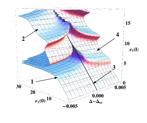
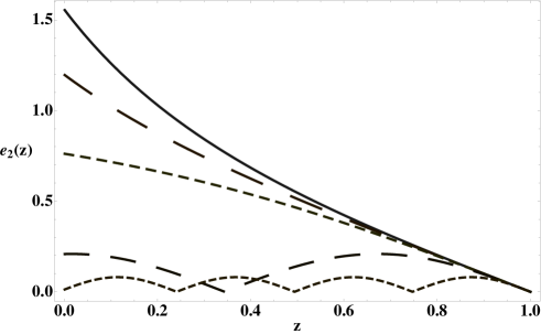
To determine the unknown parameter $m_{1}=e_{1}(l)$, Eq.(28) needs to be solved numerically. The analysis of the $e_{1}(l)$ dependence on $e_{10}$ and $\Delta$ shows that with increasing phase mismatch from $0$ to $\Delta_{cr}$, all branches (physical and nonphysical) shift upwards and nonphysical branches change their shapes. Fig. 5 shows the dependence of the output field amplitude $e_{1}(l)$ at fundamental frequency on $e_{10}$ near the critical value of phase mismatch $\Delta_{cr}$. Sheet, labeled as “1”, corresponds to the physical branch, while sheet labeled as “2” represents the first nonphysical branch. Other nonphysical sheets are located above nonphysical sheet “2” shown on Fig. 5. The spatial distribution of $e_{1}(\zeta)$ and $e_{2}(\zeta)$ can be found by substitution of the solution of the Eq. (28) ($m_{1}$) in Eqs. (26) and (27). We found that all solutions $e_{1}(\zeta)$ and $e_{2}(\zeta)$ are monotonically decreasing in $\zeta$. An example of $e_{2}(\zeta)$ at $\Delta=\Delta_{cr}/2$ is shown in Fig. 6).

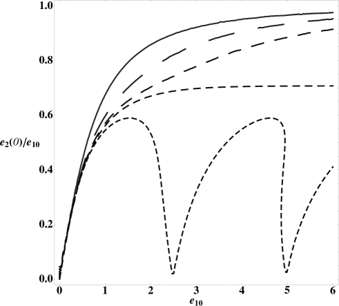
The conversion efficiency $\alpha=e_{2}(l)/e_{10}$ as a function of the input amplitude $e_{10}$ is presented in Fig. 7. As one can observe, $\alpha$ is approaching its asymptotic value $\alpha=1$ in slower fashion for larger values of $|\Delta|$.

Figure 6: The dependence of second harmonic’s amplitude $e_{2}(\zeta)$ on the $\zeta$ with different values of phase mismatch(the solid curve: $\Delta=0$, large dashed curve $\Delta=2m_{1}$, small dashed curve: $\Delta_{cr}=4m_{1}$, intermediate dashed curve: $\Delta=10m_{1}$ , doted curve: $\Delta=25m_{1}$).

IV.1.2 Critical mismatch

When the value of phase mismatch is critical $|\Delta|=\Delta_{cr}$, the roots $P_{2c}=P_{2b}=\Delta_{crit}^{2}/16=m_{1}^{2}$ and the discriminant of the Weierstrass function is zero. In this case, the function $\wp(\textit{l}-\zeta;g_{2},g_{3})$ can be represented in terms of hyperbolic functions. Thus the Eqs. (26) and (27) take the form:

$$e_{1}(\zeta)=\sqrt{m_{1}^{2}+e_{2}^{2}(\zeta)}$$ (29)

$$e_{2}(\zeta)=m_{1}\tanh{(m_{1}(\textit{l}-\zeta))}$$ (30)

and the transcendental equation for $m_{1}$ reads as

$$e_{10}^{2}=m_{1}^{2}\left(1+\tanh^{2}{(m_{1}\textit{l})}\right)$$ (31)

The numerical solution of Eq. (31) is shown in Fig.5 (line “3”). Observe that at large values of $e_{10}$, the solution of Eq. (31) is proportional to $e_{10}$ ($m_{1}\approx e_{10}$). Therefore, at large values of $e_{10}$ the conversion efficiency $\alpha\rightarrow\tanh(le_{10})$ is always less then one while in the subcritical regime $\alpha\rightarrow 1$ (see Fig. 7).

IV.1.3 Overcritical mismatch

At large mismatch values, when $|\Delta|>\Delta_{cr}$, roots of (24) are real. In this case it is convenient to represent $\wp(\textit{l}-\zeta;g_{2},g_{3})$ in terms of Jacobi elliptic $sn$ function Shabat:51 . Eqs (26) and  (27) can be represented as

$$e_{1}(\zeta)=\sqrt{m_{1}^{2}+e_{2}^{2}(\zeta)}$$ (32)

$$e_{2}(\zeta)=\sqrt{P_{2b}}~{}\mathrm{sn}\left[\sqrt{P_{2c}}(\textit{l}-\zeta),\gamma\right],$$ (33)

here $\gamma=\sqrt{P_{2b}/P_{2c}}$, and the equation for $m_{1}$ takes the following form:

$$e_{10}^{2}=m_{1}^{2}+P_{2b}~{}\mathrm{sn}^{2}\left[\sqrt{P_{2c}}\textit{l},\gamma\right]$$ (34)

Figure 7: Dependence of conversion efficiency $\alpha=e_{2}(0)/e_{10}$ on input field amplitude $e_{10}$ with different values of phase mismatch $\Delta$: Solid curve $\Delta=0$; large dashed curve $\Delta=3.5m_{1}$; dashed curve $\Delta=3.9m_{1}$; small dashed curve $\Delta_{cr}=4m_{1}$; doted oscillation curve $\Delta=4.5m_{1}>\Delta_{cr}$

The sheet corresponding to solutions of (34) is labeled in Fig. 5 as “4”. In contrast to the subcritical regime, all solutions in this case are represented by a single sheet. This sheet has folds. Hence the intersection of this sheet with plane corresponding to $\Delta=const$ gives multivalued dependance of $e_{1}(l)$ on $e_{10}$. This dependance for two different values of $\Delta$ is shown in Fig. 8.

In the supercritical regime the second harmonic field experiences spatial periodic oscillations with period $4\textbf{K}(\gamma)$ (see Fig. 6). The distance between neighboring zeros $\tilde{\zeta}$ of the amplitude of second harmonic is determined by the following formula:

$$\tilde{\zeta}=\frac{2\textbf{K}(\gamma)}{\sqrt{P_{2c}}}$$ (35)

If the slab length satisfies the condition $l=n\times\tilde{\zeta}$ ($n=1,2,3\ldots$), then the amplitude of the second harmonic wave is zero at the both ends of the slab (zero conversion efficiency). Therefore such slab is transparent for a pump wave. A plot of the transmission coefficient $\Im=e_{1}(\textit{l})^{2}/e_{10}^{2}$ as function of $e_{10}$ is shown in Fig.9. The transmission coefficient is equal to $1$ at the points labeled as “1”, “2”, $\ldots$ (transmission resonances). The spatial distribution of the fundamental and second harmonic fields corresponding to the transmission resonance at the point “1” (see Fig.9) is shown in Fig.10.

Figure 8: The dependence of the output field amplitude $e_{1}(l)$ at fundamental frequency on $e_{10}$. Solid curve $\Delta=4.1m_{1}$, dashed curve $\Delta=4.5m_{1}$

Figure 9: Dependence of the transmission coefficient $\Im$ on pumped field amplitude $e_{10}$. $\Delta=4.2m_{1}$

Figure 10: Spatial distribution of the intensities $e_{1}^{2}(\zeta)$ (solid curve) and $e_{2}^{2}(\zeta)$ (dashed curve) inside the slab

V Conclusion

We considered second harmonic generation in negative index materials. Specifics of this process is in the negative value of refractive index for the pump wave and the positive value for second harmonic. This led to important features which are different from the case of second harmonic generation in conventional dielectrics. The main difference is in the existence of nonzero critical values of the phase mismatch. If the absolute value of phase mismatch is below critical, then the field intensities are monotonically decaying along the sample. When the absolute value of phase mismatch exceeds a critical value, monotonic decay of intensities transforms to a spatial periodic oscillations. Note, that in the conventional case the critical value of phase mismatch is zero.

Another important feature is the dependance of conversion efficiency on the amplitude of the incident pump wave. When the absolute value of phase mismatch is below critical value, then the conversion efficiency asymptotically approaches 100% at large values of the incident pump wave amplitude. It should be stressed that in this case the asymptotic value of conversion efficiency does not depend on the phase mismatch value. The phase mismatch affects only the rate of approaching of conversion efficiency to its asymptotic value. When the phase mismatch is exactly equal to critical value, then the asymptotic value of conversion efficiency experiences a jump to a value which is less than 100%. When the absolute value of phase mismatch is above critical value, the conversion efficiency becomes an oscillatory function of the incident pump wave amplitude.

Finally, we found that the dependance of output amplitude of the pump wave on its input amplitude is single valued if the absolute value of phase mismatch is below critical and becomes multi-valued in the opposite case.

References

- (1) R. Shelby, D. R. Smith and S. Schultz, Science, 292, (2001) 77.
- (2) V. M. Shalaev, W. Cai, U. K. Chettiar, H. Yuan, A. K. Sarychev, V. P. Drachev, A. V. Kildishev, Opt. Lett. 30, 3356 (2005).
- (3) S. Zhang, W. Fan, C. Panoiu, K. J. Malloy, R. M. Osgood, S. R. Brueck, Phys. Rev. Lett. 95, 137404 (2005).
- (4) A. K. Sarychev and V. M. Shalaev, Electrodynamics of Metamaterials, World Scientific, Singapore, 2007
- (5) Y.R. Shen The principles of non-linear optics (John Wiley Sons, New York, Chicester, Brisbane, Toronto, Singapore, 1984).
- (6) R.W. Boyd, Nonlinear optics,(Academic Press, Boston 1992).
- (7) N. M. Litchinitser, I. R. Gabitov, A.I. Maimistov, V.M. Shalaev Negative Refractive Index Metamaterials in Optics.
- (8) Popov, A. K., Shalaev, V. M., 2006, Negative-Index Metamaterials: Second-Harmonic Generation, Manley-Rowe Relations and Parametric Amplification, Appl. Phys. B.
- (9) J.A. Armstrong, N. Bloembergen, J. Ducuing and P.S. Pershan , Interactions between light waves in a nonlinear dielectric, Phys. Rev. 127, 1918 1939, 1962.
- (10) V.M. Agranovich, Y.R. Shen, R.H. Baughman, and A.A. Zakhidov, Phys. Rev. B: Condens. Matter Mater. Phys., 69, 165 112, (2004)
- (11) V.M. Agranovich and Yu.N. Gartshtein, Usp. Fiz. Nauk, 176, p. 1051, (2006)
- (12) V.P. Drachev, W. Cai, U. Chettiar et al., Laser Phys. Lett., 3, p. 49, (2006)
- (13) W. Cai, U.K. Chettiar, H.-K. Yuan et al., Opt. Express, 15, p. 3333, (2007)
- (14) I.V. Shadrivov, A.A. Zharov and Yu.S. Kivshar, J. Opt. Soc. Am. B: Opt. Phys., 23, p. 529, (2006)
- (15) A.K. Popov, V.V. Slabko and V.M. Shalaev, Laser Phys. Lett., 3, p. 293, (2006)
- (16) A.K. Popov and V.M. Shalaev, Appl. Phys. B, 84, p. 131, (2006).
- (17) A. K. Popov and Vladimir M. Shalaev, Opt. Lett. 31, 2169-2171 (2006)
- (18) A.K. Popov and V.M. Shalaev, Journal Applied Physics B: Lasers and Optics Publisher 84, 131-137 (2006)
- (19) A.I. Maimistov, I.R. Gabitov and E.V. Kazantseva, Opt. Spektrosk., 102, p. 99 (2007) [Opt. Spectrosc. (Engl. Transl.), 102, p. 90].
- (20) Lavrentev M.A., Shabat B.V. Complex analysis, Moscow, 1951 (in russian).
- (21) Whittaker ET, Watson G. A course of modern analysis. Cambridge: Cambridge University Press; 1988.