Interference of Fano-Rashba conductance dips

Abstract

We study the interference of two tunable Rashba regions in a quantum wire with one propagating mode. The transmission dips (Fano-Rashba dips) of the two regions either cross or anti cross depending on the distance between the two regions. For large separations we find Fabry-Pérot oscillations due to the interference of forwards and backwards propagating modes. At small separations overlapping evanescent modes play a prominent role, leading to an enhanced transmission and destroying the conductance dip. Analytical expressions in scattering-matrix theory are given and the relevance of the interference effect in a device is discussed.

1 Introduction

The Rashba interaction is a spin-orbit coupling present in two-dimensional electron gases (2DEG’s) confined by asymmetric potentials in the perpendicular direction [1]. It has attracted a lot of attention, mostly due to its tunability by electrical gating [2, 3]. Indeed, a controlled spin-orbit (SO) coupling offers exciting possibilities to manipulate electron spin and current in, so-called, spintronic devices [4]. A paradigm of spintronic device, the spin transistor suggested by Datta and Das [5], relies on the Rashba-induced spin precession as an electron propagates in a semiconductor quantum wire. The feasibility of this working principle has been demonstrated in experiment only recently [6].

Besides the constant-spin-orbit case, situations where the Rashba coupling acting on a 2DEG is inhomogeneous in space have been theoretically addressed analyzing interface-induced effects such as, e.g., spin accumulation, beam focussing and “spin optics” [7, 8, 9, 10, 11]. A finite SO region in a 2DEG has been shown to contain bound states purely induced by the spin-orbit coupling [12]. In a quantum wire, a finite SO region produces quasibound states that quench the wire’s conductance at specific energies, i.e., dips appear in the conductance plateau for a given number of propagating modes. In Ref. [13], Sánchez and Serra discussed how this mechanism can be understood in terms of the well known Fano resonances of atomic physics [14], suggesting the name Fano-Rashba resonance for this conductance dips. Fano-Rashba dips have been studied in presence of disorder [15, 16] and under the influence of magnetic fields [17]. Recently, a review on Fano resonances in nanoscale structures has also been published [18].

Our aim in this work is to study the interference of the Fano-Rashba conductance dips of two sequential SO regions in a quantum wire, separated by a distance $d$ (see Fig. 1). Similar SO modulations, named Rashba superlattices, have been studied in Ref. [19]. Independently tuning $\alpha_{1}$ and $\alpha_{2}$, the Rashba intensities of the two regions, the two conductance dips can be brought in closed proximity to each other. We will show that for large separations $d$ the two dips can cross, while for small $d$’s an avoided crossing of the dips is observed. This is reminiscent of the von Neumann-Wigner crossing rule of molecular levels [20]. In our case, the coupling is mediated by evanescent modes around each SO region. If $d$ is larger than the range of the evanescent modes, the dip-dip coupling vanishes and a crossing behaviour is seen. On the other hand, for small $d$’s avoided crossing of the two dips is obtained when transport is enhanced due to transmission from the first to the second region through evanescent modes.

The relevance of evanescent modes in confined (quasi-1D) transmission is well known [21, 22, 23, 24]. For Dirac-delta impurities, Bagwell [21] showed that the dependence of the transmission on the separation between scatterers has two clear regimes: a) a Fabry-Pérot regime for large separations where the dominant mechanism is the interference between forwards and backwards propagating modes between scatterers; b) at small separations a regime where transmission occurs predominantly through evanescent modes. This is precisely the physical scenario we have sketched above for the interference of two Fano-Rashba dips. It is also worth stressing that transmission through evanescent modes between scatterers has been proved relevant for the Anderson localization of disordered wires [22].

In this work we will present numerical calculations of a quantum wire’s transmission in the presence of two tunable Rashba regions. The physical analysis of the relevant mechanisms will be performed using scattering matrix theory, composing the matrices of successive scatterers. As in Ref. [22], we have considered a generalized formulation of scattering-matrix theory where propagating and evanescent modes are treated on an equal footing. Truncating to different numbers of evanescent modes we study quantitatively their relevance, as a function of the distance between the two Rashba regions. For the case of only one propagating mode, we obtain an analytical formula for the transmission. Finally, the use of sequential Rashba regions as a spin-orbit-controlled device is discussed.

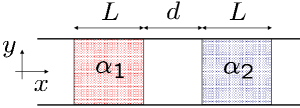
Figure 1: (Color online) Sketch of the quantum wire with two tunable Rashba regions of length $L$ separated by a distance $d$.

2 Physical system and model

We consider a 2DEG with a parabolic confinement along $y$ and free motion along $x$ described by the Hamiltonian

$${\cal H}_{0}=\frac{p_{x}^{2}+p_{y}^{2}}{2m}+\frac{1}{2}m\omega_{0}^{2}y^{2}\;.$$ (1)

An inhomogeneous Rashba interaction of type

$${\cal H}_{R}=\alpha(x)\left(p_{x}\sigma_{y}-p_{y}\sigma_{x}\right)-i\frac{\hbar}{2}\alpha^{\prime}(x)\sigma_{y}\,,$$ (2)

is active in the quantum wire. The Rashba intensity $\alpha(x)$ is assumed to vanish everywhere except in two separate regions where it takes the constant values $\alpha_{1}$ and $\alpha_{2}$. A sketch of the physical system is given in Fig. 1. More precisely,

$$\alpha(x)=\alpha_{1}{\cal F}_{x_{1},L}(x)+\alpha_{2}{\cal F}_{x_{2},L}(x)\;,$$ (3)

where

$${\cal F}_{x_{0},L}(x)=\frac{1}{1+e^{(x-x_{0}-L/2)/\sigma}}-\frac{1}{1+e^{(x-x_{0}+L/2)/\sigma}}$$ (4)

describes a square barrier of length $L$ centered at $x_{0}$. In Eq. (4) the length $\sigma$ is introduced to model smooth space transitions with $\sigma\ll L$. The distance between the two Rashba regions defined by Eq. (3) is $d=x_{2}-x_{1}-L$ and it is always assumed $d>0$ to avoid overlapping. Experimentally, the Rashba interaction can be controlled with gate electrodes modifying the $z$-asymmetry of the quantum well hosting the 2DEG [2, 3]. Our model would thus require an independent tuning of the gates defining $\alpha_{1}$ and $\alpha_{2}$. Notice also that no electrostatic in-plane effects, other than the lateral potential $m\omega_{0}^{2}y^{2}/2$ are contained in the model.

The transverse modes of Eq. (1) are characterized by

$$\begin{array}[]{rcl}\left(\frac{p_{y}^{2}}{2m}+\frac{1}{2}m\omega_{0}^{2}y^{2}\right)\phi_{n}(y)&=&\varepsilon_{n}\phi_{n}(y)\;,\\ \varepsilon_{n}&=&\left(n-\frac{1}{2}\right)\hbar\omega_{0},\quad(n=1,2,\dots)\;.\end{array}$$ (5)

The 2D electron wave function $\Psi(x,y,\eta)$ where $\eta=\uparrow,\downarrow$ is the spin variable, fulfills the Schrödinger equation for a given energy $E$

$$({\cal H}-E)\Psi(x,y,\eta)=0\;.$$ (6)

As in Ref. [13] we expand the wave function in transverse and spin eigenmodes

$$\Psi(x,y,\eta)=\sum_{n=1,2,\dots,s=\pm}{\psi_{ns}(x)\phi_{n}(y)\chi_{s}(\eta)}\;,$$ (7)

where $\chi_{s}(\eta)$ are eigenspinors in $y$ direction. Projecting we find the equation for each channel amplitude $\psi_{ns}(x)$,

$$-\frac{\hbar^{2}}{2m}\psi^{\prime\prime}_{ns}(x)+(\varepsilon_{n}-E)\psi_{ns}(x)+\sum_{ns}{\langle ns|{\cal H}_{R}|n^{\prime}s^{\prime}\rangle\psi_{n^{\prime}s^{\prime}}(x)} = 0\;.$$ (8)

The matrix element of the Rashba interaction $\langle ns|{\cal H}_{R}|n^{\prime}s^{\prime}\rangle$ in the $y\eta$ space is the only source of interchannel coupling. More specifically, the $p_{x}\sigma_{y}$ contribution to ${\cal H}_{R}$ is fully diagonal and only the $p_{y}\sigma_{x}$ induces a coupling between $\psi_{ns}(x)$ and the splin-flipped neighbouring bands $\psi_{n\pm 1\bar{s}}(x)$. Next section contains the numerical results by solving the system of coupled equations (8) with the quantum transmitting boundary method. The reader is addressed to Ref. [25] and references therein for more details on the numerical algorithm. We will consider one propagating mode, $\varepsilon_{1}<E<\varepsilon_{2}$, and focus our attention on the system conductance, determined by the quantum transmission with the help of Landauer formula $G=Te^{2}/h$, where $T$ is the total quantum transmission obtained after summing the modulus squared of the transmission amplitudes for the two spin channels $T=\sum_{ss^{\prime}}{|t_{1s,1s^{\prime}}|^{2}}$.

3 Results

3.1 Numerical

This subsection presents the transmission of the system obtained numerically with the method of Ref. [25]. The total number of modes, both propagating and evanescent, in the linear system of equations (8) is taken to be large enough to yield converged results. We focus on the Fano-Rashba conductance dips for a fixed $\alpha_{1}$ and varying $\alpha_{2}$. Dark regions represent the position of the conductance dips. The figure clearly shows that for large separation between the two Rashba regions there is a crossing of the two dips that evolves to an anti crossing for small values. Remarkably, for an intermediate distance ($d=4\ell_{0}$) the two dips are in a perfectly destructive interference, leading to a high conductance at the position where the crossing would normally occur. We also notice that for very short distances the dips become highly asymmetric, with one of them clearly dominating the other. The scenario presented in Fig. 2 can be interpreted in terms of a $d$-dependent dip-dip coupling: vanishing for large distances (crossing behaviour) and increasing at small $d$’s (anti crossing). We present in what follows evidence proving that the quantum wire evanescent modes mediate this coupling using, for this purpose, a scattering matrix formalism.

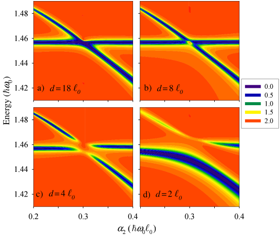
Figure 2: (Color online) Conductance in units of $e^{2}/h$ as a function of $\alpha_{2}$ and $E$ for a fixed $\alpha_{1}=0.3\hbar\omega_{0}\ell_{0}$, $L=8\ell_{0}$ and $\sigma=0.1\ell_{0}$. Each panel corresponds to a different value of $d$, the distance between the two Rashba regions. The wire parabolic confinement fixes our energy $\hbar\omega_{0}$ and length unit $\ell_{0}=\sqrt{\hbar/m\omega_{0}}$. Dark (bright) colour indicates low (high) conductance.

3.2 Scattering matrix theory

Scattering phenomena in quantum mechanics with coherent wave functions are described by scattering matrix theory. For a single scatterer there is a matrix of complex numbers relating the flux amplitudes of outgoing channels $\{b_{c,ns}\}$ to those of incoming ones $\{a_{c,ns}\}$, where we introduced a “contact” label $c=\ell,r$ (referring to left $\ell$ or right $r$), while $ns$ are indicating transverse mode and spin as before. Namely,

$$\left(\begin{array}[]{c}\sqrt{k_{n}}b_{\ell,ns}\\ \sqrt{k_{n}}b_{r,ns}\end{array}\right)=\left(\begin{array}[]{cc}r_{ns,n^{\prime}s^{\prime}}&t^{\prime}_{ns,n^{\prime}s^{\prime}}\\ t_{ns,n^{\prime}s^{\prime}}&r^{\prime}_{ns,n^{\prime}s^{\prime}}\\ \end{array}\right)\left(\begin{array}[]{c}\sqrt{k_{n^{\prime}}}a_{\ell,n^{\prime}s^{\prime}}\\ \sqrt{k_{n^{\prime}}}a_{r,n^{\prime}s^{\prime}}\end{array}\right)\;.$$ (9)

As usual, a sum is implied for repeating indexes in Eq. (9) and the factors $\sqrt{k_{n}}$ take into account the channel flux by introducing the channel wavenumbers

$$k_{n}=\frac{\sqrt{2m(E-\varepsilon_{n})}}{\hbar}\;.$$ (10)

The idea underlying scattering theory in quasi-1D transmission is that the wave function in the $c=\ell$ or $c=r$ regions, where the scatterer is no longer active, is given in terms of channel amplitudes and wavenumbers as

$$\Psi_{c}(x,y,\eta) = \sum_{ns}{a_{c,ns}\,\phi_{n}(y)\chi_{s}(\eta)\,e^{is_{c}k_{n}(x-x_{c})}}$$ (11)

$$+ \sum_{ns}{b_{c,ns}\,\phi_{n}(y)\chi_{s}(\eta)\,e^{-is_{c}k_{n}(x-x_{c})}}\;.$$

In Eq. (11) we have introduced the notation $s_{\ell}=1$ and $s_{r}=-1$ and $x_{c}$ is indicating the position where the scatterer becomes inactive for contact $c$.

For our present purposes, it is essential to realize that the number of channels $\{ns\}$ in Eqs. (9) and (11) is, in principle, infinite [22]. For a given energy $E$ part of these channels will be propagating ($E\geq\varepsilon_{n}$) and the rest will have an evanescent character. The intrinsic distinction between propagating and evanescent characters is that the wavenumber, Eq. (10), is real in the former and purely imaginary in the latter. The physical meaning becomes obvious when looking at the $x$-dependence of Eq. (11). Though infinite, the number of evanescent channels is truncated in practice and fast convergence is usually obtained.

3.3 Sequential scatterers

Assuming the scattering matrix of one scatterer is known, the solution for two identical scatterers can be obtained by adequately composing the matrices of each scatterer. This procedure only requires to realize that the right output from the first scatterer becomes left input for the second and vice versa. We need to label now the amplitudes with the “impurity” index $i=1,2$ as $\{a^{(i)}_{c,ns},b^{(i)}_{c,ns}\}$. Assuming that all the input coefficients vanish except that of mode $n=1$ with spin $s_{i}$, $a^{(1)}_{\ell,1s_{i}}=1$, the linear system for the output coefficients reads

$$\left\{\begin{array}[]{rcl}b^{(1)}_{\ell,ns}-\displaystyle\sum_{n^{\prime}s^{\prime}}{t^{\prime}_{ns,n^{\prime}s^{\prime}}\,e^{ik_{n^{\prime}}d}\,b^{(2)}_{\ell,n^{\prime}s^{\prime}}}&=&r_{ns,1s_{i}}\;,\\ b^{(1)}_{r,ns}-\displaystyle\sum_{n^{\prime}s^{\prime}}{r^{\prime}_{ns,n^{\prime}s^{\prime}}\,e^{ik_{n^{\prime}}d}\,b^{(2)}_{\ell,n^{\prime}s^{\prime}}}&=&t_{ns,1s_{i}}\;,\\ b^{(2)}_{\ell,ns}-\displaystyle\sum_{n^{\prime}s^{\prime}}{r_{ns,n^{\prime}s^{\prime}}\,e^{ik_{n^{\prime}}d}\,b^{(1)}_{r,n^{\prime}s^{\prime}}}&=&0\;,\\ b^{(2)}_{r,ns}-\displaystyle\sum_{n^{\prime}s^{\prime}}{t_{ns,n^{\prime}s^{\prime}}\,e^{ik_{n^{\prime}}d}\,b^{(1)}_{r,n^{\prime}s^{\prime}}}&=&0\;.\end{array}\right.$$ (12)

Equation (12) can be viewed as a sparse linear system for the unknowns $\{b^{(i)}_{c,ns}\}$. It can be solved with standard sparse numerical routines for a fairly large number of evanescent modes [26, 27]. Reversely, for just one propagating mode, or one propagating and one evanescent mode, analytical solutions can be given that recover known results for the composition of scatterers (see Appendix). Of all the output amplitudes of Eq. (12), we are interested in the total transmission amplitude $t_{1s_{o},1s_{i}}\equiv b^{(2)}_{r,1s_{o}}$, representing the right output from impurity 2 in channel $1s_{o}$ corresponding to a left input in impurity 1 in channel $1s_{i}$, $a^{(1)}_{\ell,1s_{i}}=1$.

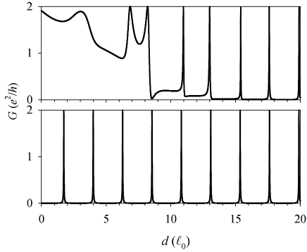
Figure 3: Conductance as a function of distance $d$ between Rashba regions for an energy $E=1.457\hbar\omega_{0}$ and $\alpha_{1}=0.3\hbar\omega_{0}\ell_{0}$ obtained with the method of scatterer composition. Upper panel is the result including evanescent modes while lower panel only considers the propagating mode.

The method of scatterer composition allows us to investigate the dependence on $d$, the distance between impurities, in an explicit way from Eq. (12). A technical point worth of stressing is that an important simplification occurs for identical scatterers placed sequentially along $x$; namely, the scattering matrix is the same for each scatterer. Figure 3 shows the result obtained as a function of $d$ for the energy and Rashba intensity of the conductance dip of Fig. 2. When evanescent modes are fully neglected (lower panel) the transmission of the system vanishes except for a sequence of very narrow, equally spaced peaks. They correspond to a Fabry-Pérot-like regime [21] with constructive interference at distances such that an exact multiple of the electron wavelength fits in between Rashba regions. This behavior changes dramatically for low distances when evanescent modes are included (upper panel): the dip is effectively destroyed by evanescent-mode transmission from the first to the second Rashba region. This effect exactly corresponds to the anti crossing seen in Fig. 2 at small distances. With the resolution of Fig. 3 upper panel, it is enough to include one evanescent mode, the contribution from higher ones being exceedingly small.

3.4 Device

The conductance dips discussed above are quite narrow and, therefore, not robust against thermal or disorder fluctuations. Their observation requires the use of very low temperatures and purely ballistic samples. It was shown in Ref. [13] that for stronger $\alpha$’s broader dips are induced at the end of the first conductance plateau. For a more robust conductance dip, in this section we analyze the effect discussed in this paper in a device in which current is controlled by manipulating the intensity of successive Rashba regions (See Fig. 4). The idea that a superlattice of this type could be of importance in practical application was already pointed out in Refs. [15, 16]. Our purpose here is to analyze this mechanism from the point of view of interference between Fano-Rashba dips through evanescent modes.

Figure 4 displays the conductance for up to 3 regions with a strong ratio $\alpha/\hbar\omega_{0}\ell_{0}$. For a single region there is a sizeable dip which, however, does dot extend all the way to zero (solid line). Adding more regions at distance $d=2\ell_{0}$ has the effect to enhance the dip forming a quasi gap amenable to practical applications (lower panels). It is remarkable how for just two or three regions with $d=2\ell_{0}$ a quasi energy gap clearly develops at the dip position $E\approx 1.25\hbar\omega_{0}$. At short distances the coupling through evanescent modes destroys the dip (upper panels) –notice, however, that a second narrow dip appears at $E\approx 1.4\hbar\omega_{0}$ for two regions (dashed line, upper left panel) but it is removed for 3 sequential regions (dash-dotted line). A device based on the tuning of $\alpha$ for sequential Rashba regions at a proper distance would not require the use of polarized leads, as compared to the Datta-Das spin transistor. Its basic shortcoming, however, is the sensitivity to the incoming electron energy which should lie in the region of the quasi gap. Increasing the number of sequential regions makes the quasi gap more robust. The distance between Rashba regions should be chosen appropriately in order to avoid destructive interference through evanescent modes.

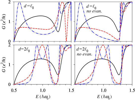
Figure 4: (Color online) Upper: Conductance as a function of energy for sequential Rashba regions, each one having $L=\ell_{0}$ and $\alpha=\hbar\omega_{0}\ell_{0}$. The different curves correspond to $1$ (solid), $2$ (dash) and $3$ (dash-dot) sequential regions. Upper and lower panels are for small and large separation $d$ between regions, respectively. For comparison, right panels show the result when evanescent channels are not included. Lower panels suggest transistor operation by tuning $\alpha$, for $E/\hbar\omega_{0}\approx 1.25$, with the OFF and ON states represented by $\alpha/\hbar\omega_{0}\ell_{0}\approx 1$ and $\approx 0$, respectively.

4 Conclusions

The interference of the Fano-Rashba dips of two successive Rashba regions in a quantum wire has been analyzed. As a function of the separation the two dips evolve from an anti crossing behaviour at large distances to a crossing when the two regions are close. The physics has been interpreted in terms of a dip-dip coupling mediated by the wire’s evanescent modes. The generalized formulation within scattering matrix theory, including evanescent and propagating modes on an equal footing, has been discussed. The numerical solution of the resulting linear equation system has been implemented. In the limit of only one or two modes analytical expressions have been given. Finally, the application to a device in which current is controlled by tuning two or three sequential Rashba regions has been discussed. A main obstacle in practice is the energy sensitivity of the Fano-Rashba dip. The conductance quasi-gap is destroyed at short distances and it becomes more and more robust when increasing the number of Rashba regions for a proper value of $d$.

Appendix A Analytical

For only two modes it is possible to obtain analytical solutions to the linear system Eq. (12). Let us assume there are only one propagating $n=1$ and one evanescent $n=2$ modes. Taking into account spin, the set of channels splits into two coupled subsets $\{1+,2-\}$ and $\{1-,2+\}$. Since both subsets are equivalent we restrict to the first one by considering incidence in mode $1+$. The transmitted output amplitude reads (spin indexes are not explicitly written to simplify notation)

$$b^{(2)}_{r,1} = \frac{t_{11}t_{11}\,e^{ik_{1}d}}{1-R_{11}-\frac{R_{12}R_{21}}{1-R_{22}}}+\frac{t_{11}R_{12}t_{21}\,e^{ik_{1}d}}{(1-R_{11})(1-R_{22})-R_{12}R_{21}}$$ (13)

$$+ \frac{t_{12}t_{21}\,e^{ik_{2}d}}{1-R_{22}-\frac{R_{12}R_{21}}{1-R_{11}}}+\frac{t_{12}R_{21}t_{11}\,e^{ik_{2}d}}{(1-R_{11})(1-R_{22})-R_{12}R_{21}}\;,$$

where we have defined

$$R_{n_{1}n_{2}} = r^{\prime}_{n_{1}1}r_{1n_{2}}e^{i(k_{1}+k_{n_{2}})d}+r^{\prime}_{n_{1}2}r_{2n_{2}}e^{i(k_{2}+k_{n_{2}})d}\;,$$ (14)

with $n_{1,2}=1,2$.

The explicit dependence on $d$, the distance between Rashba regions, is contained in Eqs. (13) and (14). To analyze the large-$d$ limit we recall that the evanescent wavenumber is purely imaginary $k_{2}=i\kappa_{2}$ ($\kappa_{2}>0$). As a result we get in that limit $e^{ik_{2}d}\to 0$ as well as $R_{12}\to 0$, $R_{22}\to 0$ and

$$R_{11} \to r^{\prime}_{11}r_{11}e^{i2k_{1}d}$$

$$R_{21} \to r^{\prime}_{21}r_{11}e^{i2k_{1}d}\;.$$ (15)

The transmitted amplitude is then

$$b^{(2)}_{r,1}=\frac{t_{11}t_{11}\,e^{ik_{1}d}}{1-r^{\prime}_{11}r_{11}e^{i2k_{1}d}}\;,$$ (16)

which is a familiar relation frequently used for single mode conductors. Equation (13) contains the analytical $d$-dependence that generalizes Eq. (16) in the presence of one evanescent channel. This causes, as shown in Fig. 3, a modification of the transmission resonances at short distances.

References

References

- [1] Rashba E I 1969 Fiz. Tverd. Tela (Leningrad) 2 1224 (1960 Sov. Phys. Solid State 2 1109)
- [2] Nitta J, Akazaki T, Takayanagi H and Enoki T 1997 Phys. Rev. Lett.78 1335
- [3] Engels G, Lange J, Schäpers Th and Lüth H 1997 Phys. Rev.B 55 R1958
- [4] Zutic I, Fabian J and Das Sarma S 2004 Rev. Mod. Phys.76 323
- [5] Datta S and Das B 1990 App. Phys. Lett. 56 665
- [6] Quay C H L, Hughes T L, Sulpizio J A, Pfeiffer L N, Baldwin K W, West K W, Goldhaber-Gordon D and de Picciotto R 2010 Nature Phys. 6 336
- [7] Khodas M, Shekhter A and Finkel stein A M 2004 Phys. Rev. Lett.92 086602
- [8] Usaj G and Balseiro C A 2004 Phys. Rev.B 70 R041301
- [9] Marigliano Ramaglia V, Bercioux D, Cataudella V, De Filippis G and Perroni C A 2004 J. Phys.: Condens. Matter16 9143
- [10] Nikolić B K, Souma S and Zârbo L P and Sinova J 2005 Phys. Rev. Lett.95 046601
- [11] Glazov M M and Sherman E Ya 2005 Phys. Rev.B 71 241312
- [12] Valin M, Puente A and Serra L 2004 Phys. Rev.B 69 153308
- [13] Sánchez D and Serra L 2006 Phys. Rev.B 74 153313
- [14] Fano U 1961 Phys. Rev.124 1866
- [15] Shen K and Wu M W 2008 Phys. Rev.B 77 193305
- [16] Wang L, Shen K, Cho S Y and Wu M W 2008 J. Appl. Phys.104 123709
- [17] Sánchez D, Serra L, Choi M S 2008 Phys. Rev.B 77, 035315
- [18] Miroshnichenko A E, Flach S and Kivshar Yu S 2010 Rev. Mod. Phys.82 2257
- [19] Zhang L, Brusheim P and Xu H Q 2005 Phys. Rev.B 72 045347
- [20] Bransden B H and Joachain C J 2003 Physics of Atoms and Molecules (London: Prentice Hall)
- [21] Kumar A and Bagwell P F 1991 Phys. Rev.B 43 9012
- [22] Cahay M, Bandyopadhyay S, Osman M A and Grubin H L 1990 Surface Science 228 301
- [23] Barbosa J C and Butcher P N 1997 Superlattices Microstruct. 22 325
- [24] Serra L, Sánchez D and López R 2007 Phys. Rev.B 76 045339
- [25] Gelabert M M, Serra L, Sánchez D and López R (2010) Phys. Rev.B 81 165317
- [26] Serra L and Choi M S 2009 Eur. Phys. J. B 71 97
- [27] 2007 HSL, a collection of FORTRAN codes for large-scale scientific computation (See http://www.hsl.rl.ac.uk)